Interactive Example-Based Terrain Authoring with Conditional Generative Adversarial Networks

HAL Id: hal-01583706

https://hal.archives-ouvertes.fr/hal-01583706v3

Submitted on 28 Sep 2017

HAL is a multi-disciplinary open access

archive for the deposit and dissemination of

sci-entific research documents, whether they are

pub-lished or not. The documents may come from

teaching and research institutions in France or

abroad, or from public or private research centers.

L’archive ouverte pluridisciplinaire HAL, est

destinée au dépôt et à la diffusion de documents

scientifiques de niveau recherche, publiés ou non,

émanant des établissements d’enseignement et de

recherche français ou étrangers, des laboratoires

publics ou privés.

Conditional Generative Adversarial Networks

Eric Guérin, Julie Digne, Eric Galin, Adrien Peytavie, Christian Wolf, Bedrich

Benes, Benoît Martinez

To cite this version:

Eric Guérin, Julie Digne, Eric Galin, Adrien Peytavie, Christian Wolf, et al.. Interactive

Example-Based Terrain Authoring with Conditional Generative Adversarial Networks. ACM Transactions on

Graphics, Association for Computing Machinery, 2017, 36 (6). �hal-01583706v3�

Generative Adversarial Networks

ÉRIC GUÉRIN,

JULIE DIGNE,

ÉRIC GALIN,

ADRIEN PEYTAVIE,

CHRISTIAN WOLF,

BEDRICH BENES,

BENOÎT MARTINEZ,

Authoring virtual terrains presents a challenge and there is a strong need for authoring tools able to create realistic terrains with simple user-inputs and with high user control. We propose an example-based authoring pipeline that uses a set of terrain synthesizers dedicated to speci�c tasks. Each ter-rain synthesizer is a Conditional Generative Adversarial Network tter-rained by using real-world terrains and their sketched counterparts. The training sets are built automatically with a view that the terrain synthesizers learn the generation from features that are easy to sketch. During the authoring process, the artist �rst creates a rough sketch of the main terrain features, such as rivers, valleys and ridges, and the algorithm automatically synthe-sizes a terrain corresponding to the sketch using the learned features of the training samples. Moreover, an erosion synthesizer can also generate ter-rain evolution by erosion at a very low computational cost. Our framework allows for an easy terrain authoring and provides a high level of realism for a minimum sketch cost. We show various examples of terrain synthesis created by experienced as well as inexperienced users who are able to design a vast variety of complex terrains in a very short time.

CCS Concepts: • Computing methodologies → Shape modeling; Additional Key Words and Phrases: Procedural modeling, Terrain generation, Deep Learning

ACM Reference format:

Éric Guérin, Julie Digne, Éric Galin, Adrien Peytavie, Christian Wolf, Bedrich Benes, and Benoît Martinez. 2017. Interactive Example-Based Terrain Au-thoring with Conditional Generative Adversarial Networks. ACM Trans. Graph. 36, 6, Article 228 (November 2017), 13 pages.

https://doi.org/10.1145/3130800.3130804

1 INTRODUCTION

Despite more than thirty years of research in terrain modeling, au-thoring virtual terrains by using contemporary techniques remains a demanding task. One reason for this di�culty is the wide vari-ety of geomorphological processes that control the terrain shape formation. Terrains are exposed for thousands of years to di�erent erosion and land-forming agents such as water erosion, varying temperatures, vegetation, that are di�cult to express by simple and versatile algorithms that could be used as editing tools. This brings

This work is supported by the project PAPAYA P110720-2659260, funded by the Fonds National pour la Societé Numérique, and the project HWD ANR-16-CE33-0001, sup-ported by Agence Nationale de la Recherche. We thank Howard Zhou for allowing us to use the DEM and sketch of Fig. 18.

© 2017 Association for Computing Machinery.

This is the author’s version of the work. It is posted here for your personal use. Not for redistribution. The de�nitive Version of Record was published in ACM Transactions on Graphics, https://doi.org/10.1145/3130800.3130804.

many important challenges, among them expressing the designer’s intent and modeling large-scale detailed terrains while allowing tight user-control. Generating a new terrain is a complex and de-manding process and it is even more complicated to do it intuitively and quickly.

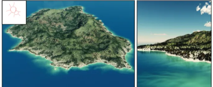
Fig. 1. A volcanic terrain generated by our method created by an inexperi-enced user from a few strokes depicting the crest lines.

A tremendous progress has been achieved in terrain modeling and the existing techniques can be categorized into procedural, simulation-based, sketch-based, and example-based. Many terrains have strong fractal features and while procedural methods allow for fast terrain generation, they often fail to provide control over the terrain features. While simulation-based methods (such as ero-sion and hydrology-based algorithms) generate geologically correct models, they often lack user control and are computationally expen-sive. Sketch-based methods provide a high level of control, but they do not generate geologically correct outputs and editing is tedious for large terrains. Existing example-based methods can generate large terrains using small examples but provide low user-control. Moreover, they replicate the exemplars, but do not easily generate new features. One important common drawback of the existing al-gorithms is that they cannot be easily applied to large-scale terrains. Recent progress in Deep Learning provided solutions to many hard problems in Computer Graphics and Vision, not only for clas-si�cation but also for synthesis. One of the most powerful gen-erative methods is the so-called Gengen-erative Adversarial Network (GAN) [Goodfellow et al. 2014] and one of its extensions, conditional GAN (cGAN).

We integrate cGANs in a fast example-based approach to real-istic terrain synthesis (Fig. 1) that is oblivious to the underlying

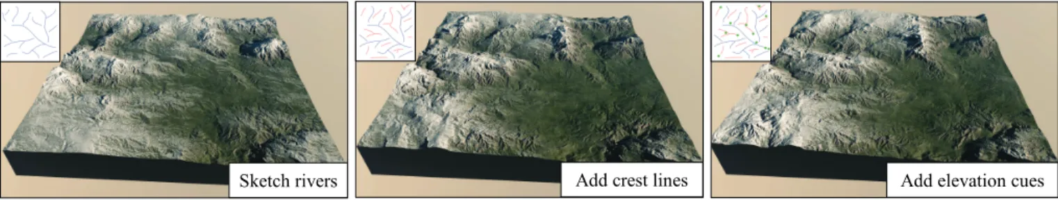
Sketch rivers Add crest lines Add elevation cues

Fig. 2. Our interactive terrain modeling framework allows the user to quickly, easily, and intuitively author realistic terrain models by using sketches of crest lines, rivers, or iso contours. Our method consists of a training step and an interactive sketching step. During the training step, we analyze a large number of terrains and extract geometric features that will serve as sketching elements. The sketches are fed to a set of cGANs which learn various generative processes. During the authoring step, the pre-trained networks are used to synthesize a terrain model that matches the input sketch and the incremental edits.

geological phenomena. Our method bridges the gap between the intuitiveness and �exibility of interactive authoring processes, while providing e�ciency and expressive power. We do not attempt to model the underlying geomorphologic phenomena, but instead we use construction by example.

The cGAN training requires large training sets and it would not be feasible to ask artists to provide hundreds of terrain sketches. Instead, we propose to extract automatically sketches from real-world terrains. These sketches combine visually important features such as crests, valleys and river networks that have clear user intu-ition and can be easily sketched. We then train several cGANs with examples built from pairs of real terrains and their automatically generated sketches. Each cGAN yields what we call a terrain syn-thesizer capable of generating the entire elevation of a terrain from input data.

Terrains are also shaped by erosion, a geomorphological pro-cess which is notoriously slow. Although GPU implementations of erosion algorithm exist, they cannot be e�ciently applied to large terrains. In our work we propose an erosion meta-simulation (simu-lation of a simu(simu-lation) by training a dedicated cGAN. This allows to apply erosion to large terrains time-e�ciently.

In our approach, the user starts the interactive editing session by providing a rough sketch of a terrain and the terrain synthesizer generates the corresponding large-scale terrain model. The result can be later modi�ed by editing the sketch, erasing and regenerating terrain parts, by our eraser synthesizer. A key feature of the entire process is its e�ciency: during the authoring session, every terrain generation takes only a few milliseconds which allows interactive feedback to the designer. An example in Fig. 2 shows the usage of our framework: starting with a river network, adding crests and elevation cues generates a real-time terrain in each step.

The main contributions of our work are threefold: 1) we propose the �rst terrain authoring pipeline driven by real world examples based on Deep Learning, 2) we present an automatic sketches gen-eration process to build learning datasets, and �nally, 3) we show that our approach can be used to learn complex natural processes, such as hydraulic erosion. We evaluated our approach by providing a large variation of landscape types (alpine mountain, volcanic is-land, canyon) and we also conducted a qualitative user study that con�rms the ease of use of our technique.

2 RELATED WORK

Terrain modeling has been a focus of computer graphics for a long time and the existing body of work can be classi�ed into proce-dural, simulation-based, and example-based techniques. We refer the reader to [Natali et al. 2013] for an overview of terrain modeling representations and to [Smelik et al. 2014] for a survey of proce-dural terrain modeling. We also brie�y review Machine Learning algorithms and especially Deep Learning algorithms.

Classical procedural methods are computationally e�cient, be-cause they usually use some kind of fractal noise that visually resem-bles real terrains. Fractals are useful for modeling terrains that are self-similar and can be observed as fresh and not eroded [Fournier et al. 1982]. Fractal interpolation was used to complete user-de�ned river networks [Kelley et al. 1988] and models generated by L-systems [Prusinkiewicz and Hammel 1993]. They were later used to generate fractal terrains constrained by user-prescribed rivers trajectories [Belhadj and Audibert 2005] and planets featuring pro-cedurally generated river networks [Derzapf et al. 2011]. A major limitation of the procedural models is their control. Fractals are de�ned by seeding a random number generator and the result is dif-�cult to predict. User control of fractal methods has been addressed by several works. In particular by de�ning terrains from feature curves such as river networks and ridges [Génevaux et al. 2013; Hnaidi et al. 2010]. Recently, Génevaux et al. [2015] introduced a hierarchical distribution tree that models the terrain as a distribu-tion of primitives that are procedurally blended, carved, and warped together. Moreover, it was quickly noticed that real terrains do not always conform to pure fractal description because they are exposed to various morphogenesis phenomena, among them erosion plays the most important role.

Simulation-based methods were introduced by the work of Mus-grave et al. [1989] who used various kinds of erosion to modify fractal terrains. Erosion algorithms were later extended by hy-draulic erosion in [Chiba et al. 1998; Nagashima 1998]. Height �elds [Cordonnier et al. 2016] are the most common representations used for erosion simulation, although layered data structures [Benes and Forsbach 2001], volumetric data [Benes et al. 2006], and smoothed particle hydrodynamics [Krištof et al. 2009] were also used. Small-scale volumetric erosion was also used to simulate cli�s [Peytavie et al. 2009]. Recently, Cordonnier et al. [2017a] used simulations in

Ge ne ra ti ve Ad ve rs ar ia l Ne tw or k T ra in in g Te rr ai n Sy nt he si ze rs 1

Curves Level sets Terrain database

Sketching with Trained synthesizers Refinement Authoring Sk et ch s yn th es iz er s S an d L Final terrain Analysis Er os io n an d er as er sy nt he si ze rs E an d R Am pl if ic at io n A 2

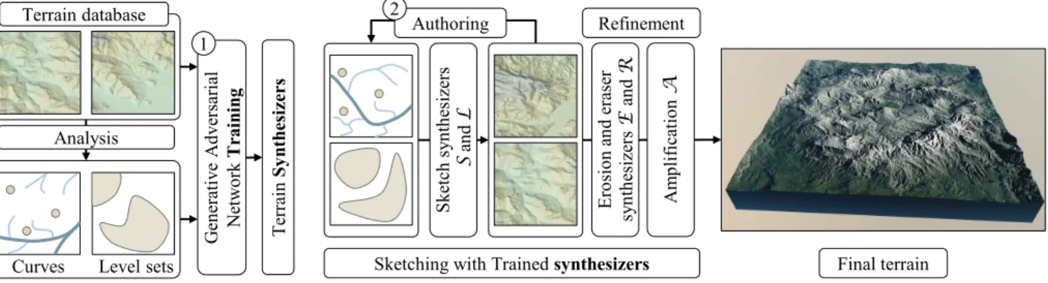
Fig. 3. Our system is a two stage process. During the training step, we analyze a large input set of example terrains and extract features such as ridge lines, river networks, levelsets or points of interest. The data and the input terrains are used to train a set of conditional Generative Adversarial Networks that learn the correlations between the terrains and the sparse data. During the interactive authoring session, the network synthesizes the terrain from the user sketch.

interactive setting to generate large-scale terrains a�ected by sub-surface tectonics. Erosion algorithms were brought at interactive frame rate by using GPUs in [Mei et al. 2007; Vanek et al. 2011]. While simulation-based algorithms generate geologically correct models, they are di�cult to control and they are computationally demanding. Moreover, it is di�cult to express a user intent by using those methods.

Example-based and user-de�ned approaches use existing terrains or user sketches to de�ne terrain models. A typical representative of the example-based methods is the approach of [Zhou et al. 2007] that uses the height �eld patches from a real terrain and combines them into a user-de�ned sketch. Various methods use high-level interac-tive inputs to de�ne terrains. Silhouettes were used to de�ne rough-ness [Gain et al. 2009, 2015] or to deform an existing terrain to create a view from a certain viewpoint [Tasse et al. 2014]. Sketch-based approaches [Gain et al. 2009; Hnaidi et al. 2010; Tasse et al. 2012] or direct interactive terrain editing [Peytavie et al. 2009] were used to de�ne terrains with a high level of control, but can generate ter-rains that are not geologically correct. Hybrid approaches combine interactive editing with simulations [Vanek et al. 2011; Šťava et al. 2008] but they are limited to small scenes. Sketch-based methods involve manual editing that can be tedious whereas example-based algorithms are limited by the input exemplars.

Machine learning has been used to generate images and other high dimensional and structured data similar to a training set for texture synthesis [Gatys et al. 2015; Kwatra et al. 2003], to generate images of a given type [Gregor et al. 2015], to predict future video frames [Mathieu et al. 2016], or to use sketches to complete pro-cedural buildings [Nishida et al. 2016]. Earlier work was based on dictionary learning [Rubinstein et al. 2010] or graphical models like MRFs/CRFs. These models are limited by the required optimization stage during decoding, resulting in scalar hidden states and low order interaction between output variables [Kwatra et al. 2003].

Neural networks overcome this limitation by dealing with struc-tured data di�erently. In the most widely used formulations, no optimization is required during decoding, which allows the model to (i) resort to a rich componential hidden state and to (ii) use complex

interactions between output variables and hidden states. Methods have been proposed which learn a direct (often convolutional) map-ping between input and output, e.g. [Dosovitskiy et al. 2015], to generate images of 3D models given object type, viewpoint and color. Probabilistic graphical models (and neural networks), such as Variational Auto-Encoders (VAE), put a strong emphasis on mod-eling stochastic latent space [Kingma and Welling 2014]. Because they are capable of modeling highly complex interactions, they can also be used to generate images [Gregor et al. 2015; Mansimov et al. 2016]. U-nets [Huang et al. 2016; Ronneberger et al. 2015] map input to output by �rst decreasing spatial resolution iteratively through a bottleneck and then restoring spatial resolution with upsampling, U-nets bene�t from additional skip-connections between layers with the same resolution.

Ulyanov [2016] used generative convolutional networks to pro-vide textures in multiple resolutions. Li and Wand [2016] used GANs to generate textures without blending, and [Zhu et al. 2016] showed how to use GANs for texturing meaningful manifolds.

The recently proposed Generative Adversarial Networks (GANs) [Goodfellow et al. 2014] are also of stochastic nature. They train two competing networks, a generator network G, able to generate new examples, and a discriminator D, able to discriminate between real examples and generated examples. The generator learns to create realistic looking images which the discriminator is unable to distinguish from the images of the training set. Although VAE provides additional control over the latent space which might help to better enforce constraints on the output, GANs currently pro-duce data of higher quality, which is due to their adversarial loss. Conditional GANs can process additional inputs which allows to learn relationships between pairs of images [Isola et al. 2016]. This has been successfully applied to digital image generation and com-pletion [Mirza and Osindero 2014; Pathak et al. 2016]. Our method also makes use of a conditional GAN to train various terrain synthe-sizers from carefully designed input samples built from real-world examples. To the best of our knowledge, deep neural networks were not used for terrain synthesis before.

3 OVERVIEW

Our method consists of a training pre-processing step and an inter-active authoring step (Fig. 3). The pre-processing step uses a set of example data-sets to produce a set of units called Terrain Synthe-sizers that are at the heart of our pipeline. A Terrain Synthesizer takes an input sketch or annotated terrain and produces an output or modi�ed terrain (Section 4).

We introduce four di�erent terrain synthesizers. The sketch-to-terrain synthesizer S creates a sketch-to-terrain from a sketch containing ridges, rivers, altitude cues or any combination of the three; the levelset-to-terrain synthesizer L turns a binary levelset image into a terrain; the eraser synthesizer R removes a user-speci�ed part of the terrain and completes it, and, �nally, the erosion synthesizer E transforms an input terrain into the corresponding eroded terrain. Because each synthesizer is specialized in a speci�c task, we need to build a set of dedicated databases from real-world examples to learn each synthesis (Section 5). The training step, performed once and for all, is particularly important since the quality and realism of the terrain produced in an authoring session is strongly correlated with the learned synthesis ability. Interestingly, one could easily add Terrain Synthesizers to the pipeline: for example to consider other kinds of sketches.

The authoring stage (Section 6) starts by loading the terrain syn-thesizers that are used during the authoring session. The input to our framework is a coarse sketch and the output is a 3D model of a terrain that is created by successive user-edits and optionally adding erosion to the �nal result. An artist will start by providing a coarse sketch features such as rivers, ridges, some altitude cues, or a combination of them. The input is given to the sketch-to-terrain synthesizer that generates a plausible terrain from it. If the result is not satisfactory, the user can re-edit the sketch and rerun the synthesis or remove parts of the terrain that will then be completed by the eraser synthesizer. After the coarse sketch is �nished, the user can erode the terrain by running the erosion synthesizer.

Once the user is satis�ed with the generated large-scale terrain, small scale details can be added by using a super-resolution tech-nique. We have used an algorithm from [Guérin et al. 2016] to add small-scale details to an existing terrain. We will refer to this method as terrain ampli�cation as it considers the information in the terrain in order to amplify it. This method is particularly well suited for the terrains generated by cGANs, because they contain coherent landforms features, but lack small scale details.

4 TERRAIN SYNTHESIZER

A key feature of our approach lies in its ability to synthesize terrains from various types of inputs. In particular, we can synthesize a terrain from di�erent kinds of sketches, complete a terrain with missing data or parts erased during interactive editing, or synthesize an eroded terrain from another input terrain. All these problems can be interpreted as learning a way to predict an output B from an input A. In our setting all terrains are represented as Digital Elevation Models (DEMs) and sketches are represented as images. Our approach builds on Conditional Generative Adversarial Net-works (cGAN) [Isola et al. 2016]. cGANs are pairs of deep netNet-works,

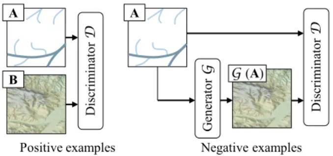
a generative network G able to generate B from A and a discrimina-tive network D able to discriminate between real pairs (A, B), i.e., data from the training set, and fake ones (A, G(A)), data generated by the network G. The name adversarial training derives from the fact that G is trained to fool D and that D tries to avoid being fooled by G. While we are mostly interested in the generative network G,

Di sc ri m in at or D

Positive examples Negative examples

Ge ne ra to r G Di sc ri m in at or D G (A) B A A

Fig. 4. Overview of the training of a cGAN: The discriminator D learns to classify between real and synthesized pairs, whereas the generator learns to fool the discriminator.

D is crucial to the learning stage because its discriminative power conditions the quality of the generator G. Indeed, the generative network can only become e�cient in producing real examples if D is e�cient at discriminating real and fake examples. Failure to do so leads to a high error on D’s side for wrong reasons: the discrimi-nators own abilities vs. the quality of the generator’s output. Thus, while G maps images to DEMs, D operates patchwise and classi�es the patches (of size 70 ⇥ 70) of the test pair as either real (=1) or fake (=0) and outputs the average over the binary decisions for all patches. If B is a real-world DEM and A its extracted sketch, the es-timated classi�cation D(A, B) should be close to 1. Conversely, the discriminator should learn to recognize a synthesized pair (A, G(A)) and tend to zero in that case. Following [Isola et al. 2016], this is captured by the following objective function:

E_{(A,B)[log D(A, B)] + EA[log(1 D(A, G(A)))].} (1) The expectation is taken over the distribution of the data (A, B). Equation (1) is maximized over the discriminator parameters. The generator should in turn learn to generate DEMs which minimize the discriminator objective (for the discriminator’s best e�ort), which turns the learning process for the generator parameters into a mini-max game:

min

G maxD E(A,B)[log D(A, B)] + EA[log(1 D(A, G(A)))].

The above adversarial objective with respect to G does not use the ground truth image B, but checks (through the discriminator) whether the generated image lies on the data manifold. In practice, this does not provide enough supervision for e�cient learning. To alleviate this lack of supervision, it is common to add a regulariza-tion term involving the ground truth image B to the objective, e.g. gradient di�erence loss [Mathieu et al. 2016] or L1regularization

kB G(A)k1, as in [Isola et al. 2016]. We chose the latter formulation.

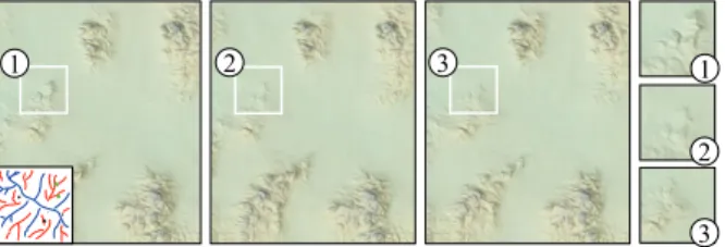
3 2 1 3 2 1

Fig. 5. The same input produces slightly di�erent outputs when executed several times. While small scale details can be di�erent, we observed that the main landforms features remain the same.

Contrary to standard GAN formulations, we do not add any noise input to the generator G, and provide noise (for stochasticity) only in the form of dropout [Krizhevsky et al. 2012], i.e. switching o� units randomly during training and testing with probability p=0.5. Thus running the synthesizer twice will yield slightly di�erent results. In our experiments, we observed that the results only slightly varied when running the synthesizer on the same input several times (Fig. 5).

The network architectures have been adapted from [Radford et al. 2016] and [Isola et al. 2016]. The generator architecture is an encoder-decoder network with an encoding part composed of a sequence of fully-convolutional layers (convolutions �lters of size 4 ⇥ 4) and resolution reductions, and a decoder composed of a se-quence of deconvolutions/upsampling. In the decoding part, each layer is thus connected to a layer of lower resolution, and additional skip-connections connect it to the encoder layer of identical res-olution (U-net). These additional connections allow to bypass the encoder-decoder bottleneck by transmitting low-level information from the input directly to the output. The number of features in the generator in the successive layers is: 64, 128, 256, 512, 512, 512, and 512. There is a single output channel storing the terrain altitude, and the number of input channels varies from one (for levelset and erosion synthesizers) to three (for sketch and eraser synthesizers). Our training follows the Image-to-Image network training [Isola et al. 2016]. We use a stochastic gradient descent with mini-batches of size one, the Adam optimizer [Kingma and Ba 2015], and the batch normalization [Io�e and Szegedy 2015]. We alternate between gradient updates of the generator and gradient updates of the dis-criminator [Goodfellow et al. 2014]. We use up to 500 epochs, which produces less artifacts in the output terrain. In order to introduce more variability to the training data, we randomly use both vertical and horizontal �ipping in addition to the standard cropping area.

5 TRAINING

Our framework needs to learn mappings from sketches to real world terrains from a set of training pairs {(A, B)} that are input to both networks (Fig. 4). Since we cannot ask an artist to generate a large database of sketch-terrain pairs, we use an automatic generation of those pairs which will govern the quality of the output terrain.

Our approach takes a real-world terrain as B, uses a dedicated algorithm that generates A, and adds the pair (A, B) to the training set. Notice that the trained synthesizers scales are bound by the scale of the training terrain datasets. In this section, we describe

our automatic training set generation. The data source and statistics about the training process are detailed in Section 7.1.

5.1 Sketch-to-terrain Synthesizer Training

Sketches can contain altitude cues, rivers, mountain ridges, or any combination of these.

River networks are obtained by simulating the water �ow on a terrain and detecting the pixels with high water accumulation. We generate river networks from the terrain elevation using a modi�ed river channel network algorithm inspired by [Tarboton et al. 1991]. We seed water over all the grid points of the terrain and simulate �ow using a modi�ed steepest descent D8 algorithm, which routes all �ow to the neighboring point to which there is the steepest downward slope [O’Callaghan and Mark 1984].

In order to prevent the water from following always the same path, we use a stochastic direction at every step where the proba-bility is proportional to the height di�erence between the current pixel and the candidate neighbor. The local minima are processed stochastically: water stuck in a local minimum leaves it with a low probability, or simply disappears. This process yields very precise river networks which may be problematic because it does not corre-spond to a real user sketch of a river network. A user would indeed provide coarse directions to the river network and would not draw every single river twist.

To alleviate this e�ect, the terrain is blurred and down-sampled before the �ow simulation and the resulting water accumulation is up-sampled to get the rivers at the initial resolution. A �nal morpho-logical operation is applied to the result in order to obtain a clean 1-pixel width skeleton. Hence the synthesizer training algorithm is provided with inputs that are coarse river directions and it learns to not strictly respect constraints, thus allowing more �exibility in the generator. Fig. 6 shows examples of terrains and their detected river network.

Rivers Crest lines Altitude cues

Fig. 6. Extracted features from di�erent input terrains.

This pre-processing has a great impact on the training, as illus-trated in Fig. 8 which shows examples of generated terrains when the dataset has not been blurred prior to the feature extraction. In this case, the extracted features that feed the training are more pre-cise and dense. In this over-constrained context, the synthesizer fails at reconstructing a terrain when the sketch in not dense enough, and even with a greater number of strokes, the generated terrain does not follow the sketch. Using blurred terrains for feature extrac-tion thus makes the synthesis more robust to imprecise and sparser sketches.

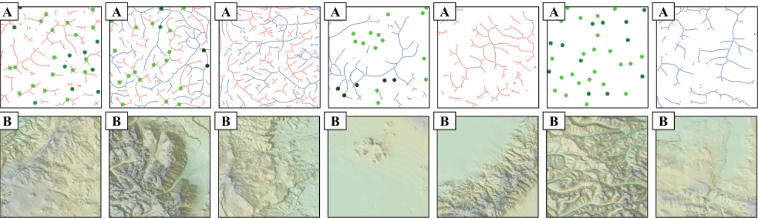
B A B A B A B A B A B A B A

Fig. 7. Di�erent kinds of multichannel sketches generated for the sketch-to-terrain training set.

2 strokes 5 strokes 39 strokes

No pr epr oc es si ng Wi th pr epr oc es si ng

Fig. 8. Comparison of synthesis results when the network is trained with features extracted on non-blurred data (top) and blurred data (bo�om). In the first case, the synthesizer needs more input sketches to reconstruct the terrain (top right). With a small number of strokes, visual artifacts appear (top le� and middle). This can be avoided when blurred terrain data are used to extract the features (bo�om row).

Ridges are detected by inverting the terrain and applying the river detection algorithm. It is the opposite operation to river detection and Fig. 6 shows examples of detected ridges.

Altitude cues are computed as a sparse set of peak and basin points over the terrain with an approximate elevation. Basin points are de�ned as points where the previous water �ow accumulated above a chosen threshold. Conversely, peak points can be de�ned in a similar way by inverting the elevation of the terrain.

The full example set is generated by providing random combi-nations of the sketch cues by using di�erent color channels of the images. We map the detected river layer to the blue channel, the ridge layer to the red channel, and the altitude to the green channel. If the sketch does not contain one of these cues, the corresponding channel is set to zero. Fig. 7 shows examples of our training pairs.

5.2 Levelset-to-terrain Synthesizer Training

As an alternative to sketching ridges, river curves, and altitude cues, the user can provide large areas of constant elevation that we call levelsets. These are provided as binary images that indicate areas in the terrain where the altitude should be above a given percentile of the altitude distribution (60% in our implementation). This levelset synthesizer serves a di�erent purpose and it cannot be used jointly with the sketch-to-terrain synthesizer. Although di�erent percentile choices could be made, we found that 60% yielded the most intuitive drawing tool. The example set for this training is easily constructed by blurring the DEMs and thresholding the altitude at the provided percentile. Fig. 9 shows three examples of the training pairs. Once again this example generation involves taking a real-world terrain B and creating the corresponding levelset input A as an entry (A, B) to the training stage.

Le ve ls et sk et ch es B A B A B A T er rai n

Fig. 9. Levelset examples. The levelset is represented in white.

5.3 Eraser Synthesizer Training

Another useful terrain design tool is an eraser synthesizer work-ing directly on the DEM, that removes parts of a terrain and infers its completion. To train this synthesizer, a real-world terrain B is modi�ed through the addition of a random number of disks with

Fig. 10. Example of an interactive authoring session performed by a professional artist: it took him a only a few minutes to design the structure of a large terrain by using ridges (le�), adjusting the generated terrain to his intent by incrementally adding rivers (middle), and defining some elevation points (right). random sizes that de�ne the missing parts. We represent the

anno-tated terrain A as a two-channel image Z , where Z denotes the elevation channel and the erasure channel. The elevation of the erased terrain part is set to 0, while the channel is set to 1. B is de�ned as the complete terrain. The pair (A, B) is added to the training database for the eraser synthesizer (Fig. 11).

Pa rt ia ll y er as ed te rr ain s B A B A B A Co m pl et e te rr ai n

Fig. 11. Eraser synthesizer training example pairs.

5.4 Erosion Synthesizer Training

The erosion examples generation proceeds slightly di�erently from the previous cases. Recall that sketch-to-terrain, levelset-to-terrain, and eraser synthesizers used real-terrains as input B and com-puted A. However, it is di�cult to �nd real-world data for a terrain and its corresponding eroded version. Instead, we create the erosion examples by taking a real-world terrain as input A and computing the corresponding data B = e(A) by simulating erosion e over A (Fig. 12).

Our approach consists in learning an algorithm that mimics the behavior of a simulation. Inspired by [Cordonnier et al. 2017b], we simulate both interleaved large-scale hydraulic and thermal erosion. Our terrain-erosion model relies on a discrete layered model repre-senting di�erent materials (bedrock, rocks and �ne grain sediments). Temperature variations and rainfall trigger aging and weathering events, such as water runo� transporting sediments, or fracture of the bedrock into rock-slides. The simulation computes the evolution of the layered model by stochastically applying a large number of events to the cells of the terrain.

Or ig in al te rr ai ns B A B A B A Er os io n

Fig. 12. Erosion synthesizer training pair examples.

Although it may appear counter-intuitive to learn a process that can be simulated, our goal is to take advantage of the e�ciency of synthesizers at run time to provide interactive feedback to the user. This method is an approximation of complex erosion phenomena that runs extremely fast as opposed to computationally demanding simulations. The idea of simulating complex and hard-to-simulate phenomena using neural network is inspired by learning computa-tionally expensive iterative processes such as image �lters [Xu et al. 2015] and style transfer [Johnson et al. 2016; Ulyanov et al. 2016].

6 AUTHORING

Interactive authoring takes place after the network training pre-processing step and it is a two-step work�ow (Fig. 3). The user �rst draws a coarse sketch and incrementally edits it by adding, modifying, and removing curves or carving level-sets. The user then re�nes the terrain by using optional erosion and ampli�cation that generates the �nal high resolution model.

6.1 Terrain Sketching

Our system uses the terrain synthesizers to generate terrains corre-sponding to the user-provided sketch at runtime. The user initially sketches a river network, a ridge network, elevation cues, or any combinations of the three and the synthesizer generates a terrain. The user may add or modify ridges, rivers, elevation cues or remove some parts of the sketch and see the results in real time as applying

Fig. 13. The iterative sketching can be used to generate complex shapes. Here the user sketches the Siggraph logo by adding a disk, carving a part of the levelset out, and finally adding details. This whole editing sequence is performed using the levelset-to-terrain synthesizer

the terrain synthesizer is very e�cient and takes around 50ms per generation.

An example in Fig. 10 shows an authoring session of an artist providing initial ridges, then adding rivers, and �nally elevation cues. Another example in Fig. 2 shows an authoring session by a novice user. The user �rst de�ned ridges, then added rivers, and modi�ed the terrain by providing a set of altitude cues.

Before erasing

Result

Fig. 14. Example of a terrain automatically generated by the eraser synthe-sizer tool that fills parts removed by the user.

A key feature of our approach is that it allows the user to use di�erent types of sketching models as input. Instead of sketching with ridge and river curves, the user can interactively edit a levelset, and use the corresponding synthesizer to generate the terrain. Fig. 13 shows three consecutive steps of an interactive level set authoring session: starting from a circular shape, the user erased the center before adding more details. This drawing tool is fast and easy to use, however it provides less control than the curve sketches. The eraser synthesizer can quickly regenerate terrains with missing parts and produces consistent models (Fig. 14).

6.2 Terrain Refinement

Terrain re�nement encompasses the processes of erosion and am-pli�cation that improve the overall realism of the generated terrain and increase its resolution.

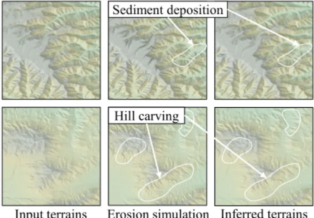
Erosion: Once the coarse sketch terrain is provided, the user can apply erosion to it. The erosion synthesizer mimics erosion algo-rithms at a very small computational cost as opposed to numerical simulations. Fig. 15 illustrates the simulated erosion on real world terrains and compares it with the learned erosion. The computation time of our trained erosion-synthesizer is three order of magni-tude faster (25ms vs 40, 000ms on a terrain of resolution 256 ⇥ 256) compared to a simulated erosion.

Input terrains Erosion simulation Inferred terrains Hill carving

Sediment deposition

Fig. 15. Simulating the erosion of a terrain comes at a very small cost at runtime.

Terrain ampli�cation: After the large-scale terrain has been gen-erated and erosion has possibly been applied, the �nal step is to add more details by using terrain ampli�cation (see Section 3). We use the patch-based ampli�cation method proposed in [Guérin et al. 2016] that builds high and low resolution patch dictionaries and decomposes the terrain onto them. Although it would be possible to also train a terrain synthesizer for the ampli�cation, this would re-quire learning several synthesizers for each resolution gain, whereas the sparse-ampli�cation performs this operation very e�ciently. Be-cause the cGANs generate coherent large-scale terrains, the terrain ampli�cation is well-suited to match terrain details to large scale terrain patches (Fig. 16).

6.3 Integration with Large Scale Terrain Modeling

A key feature of our approach is its ability to analyze input DEMs and generate sketch representations which can be used as input data

Sketching

Initial setup Generated terrain 32×32 km2

4×4 km2

Patch analysis Final rendering

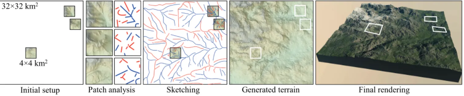
Fig. 17. Our method can generate terrains from sketches that have vast empty areas. In the initial setup, three small terrain patches of 4 ⇥ 4 km2were carefully authored and located by the designer on the large empty square terrain of size 32 ⇥ 32 km2. The analysis of the patches produced the initial local set of local ridges, rivers, and elevation landmarks, which were completed by user-defined sketches over the remainder of the domain. The terrain was automatically generated by the sketch-synthesizer S, and the patches blended with the terrain.

Synthesizer output 4x amplified terrain Fig. 16. Comparison between a synthesized terrain before (le�) and a�er amplification (right). Terrain amplification process introduces details without breaking the landform features generated by the synthesizer as can be seen in the image inset.

in the synthesizers S. Our method enables artists to generate large scale terrains featuring some speci�c regions that they authored in full detail in a seamless fashion. The overall process proceeds in three steps (Fig. 17). First, given several high-resolution input DEM patches Akembedded in a larger domain , we down-sample

and analyze them to produce their corresponding low-resolution curve or levelset sketches Bk. The user then completes the coarse

sketch over the remainder of the domain ([kAk) to get a new

representation eB. Finally, we generate the terrain A from eB and locally smoothly blend it with the prescribed patches Ak.

The analysis of the features of the detailed input patches allows us to obtain a large scale DEM whose major landform features are consistent with the prescribed patches’ ones. Therefore, the �nal blending, although simple and straightforward, generates a coherent DEM. Fig. 17 shows an example of our high level and very e�cient authoring approach. The professional artist created the 32 ⇥ 32km2

terrain featuring three speci�c landforms in less than 15 minutes.

7 RESULTS AND DISCUSSION

Generation of the training database has been implemented in Matlab®

and C++ and interfaced with TensorFlow for the Deep Learning part. We adapted the cGAN code provided by the authors of [Isola et al. 2016] to process DEM data. Training was performed on a NVidia®

Titan X graphics card with 12 Gb of memory clocked at 1.076 Ghz. Our interactive editing application was implemented in C++ and uses Qt and OpenGL for rapid previsualization. Interactive editing

performed on a standard desktop computer equipped with an Intel Core i7 CPU clocked at 3.4 GHz and with a NVidia®_{GTX 970. For}

visualization purposes, we added a procedural texture to our synthe-sized terrains. The photorealistic landscape images were rendered with the Vue®_{software. Unless stated otherwise, all high quality}

results use ampli�cation.

7.1 Database and training

Our real-world terrain database includes DEMs extracted from USGS Earth explorer. We used 35 patches of one square degree at a preci-sion of one arc-second taken from NASA SRTM. Each patch consists of a 3, 600⇥3, 600 resolution grid and each cell represents horizontal area of approximately 30 ⇥ 30 meters. We used 16 bits gray-scale in our implementation with a vertical resolution of 1m. Table 1 reports statistics for generating the di�erent databases and training the network.

Synthesizer Database creation Training_time Size Time

Sketch-to-Terrain 525 0:22 6:25 Levelset-to-Terrain 525 0:01 6:24 Eraser 500 0:01 5:48 Erosion 1400 15:13 6:54 Table 1. Timings (in hours) for the learning of terrain synthesizers.

The structure of the generator network is linked to the input terrain resolution, therefore all generated terrains will have the same resolution. Because of the fully-convolutional nature of the synthesizer, we are able to generate terrains from sketches of arbi-trary size. While the spatial resolution will remain unchanged (i.e., the pixel size will represent the same distance), the total size of the synthesized terrain can be larger. The only limitation of this process is the amount of GPU memory. In our implementation, we were able to synthesize terrains up to a resolution of 1024 ⇥ 1024.

7.2 Comparisons

In this section, we compare our method to other sketching tools, and evaluate the performance of our erosion synthesizer with respect to physically-based simulations

Several terrain sketching algorithms have been proposed in com-puter graphics. Zhou et al. [2007] proposed an example-based ter-rain authoring method based on texture synthesis techniques that generates terrains by combining patches from an input sketch and mountain range style image. Here we reproduce the lambda-shaped mountain range from their work that was sketched as a ridge with-out any additional information (Fig. 18). We used the sketch-to-terrain synthesizer on the sketch to generate the �nal sketch-to-terrain. It is important to note that our cGAN-based method allows for an interactive editing and does not require any input patches from the terrain. The features obtained by [Zhou et al. 2007] are slightly sharper than ours. We obtain similar small-scale sharp ridges and faults when completing our deep-learning-based terrain generation with ampli�cation.

Example-based Our method

Fig. 18. Comparison between the example-based method of [Zhou et al. 2007] and our method.

Hnaidi et al. [2010] proposed a terrain sketching approach that also uses sketches of ridges and rivers networks to synthesize a terrain using di�usion. An important limitation of this method lies in the amount of information that is required to generate the terrain: rivers and ridges should be precisely sketched and their elevations should be prescribed (Fig. 19). In contrast, our approach generates realistic terrains even from coarse sketches, because the synthesizers learned to generate more details from less input infor-mation. Without any derivative constraints on the ridges, Hnaidi et al.[2010] amounts to a simple heat di�usion yielding unrealistic smooth plateaus (Fig. 19).

Sketch synthesizer Diffusion

Fig. 19. Comparison between the di�usion method of [Hnaidi et al. 2010] (le�) and our sketch synthesizer (right). Without additional gradient in-formation and noise parameters, the di�usion-based method produces unnatural smooth terrains.

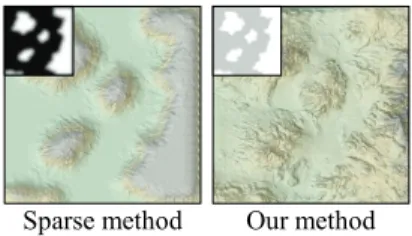
We further compare with the work [Guérin et al. 2016] (Fig. 20). The input is a levelset binary image that is fed to the leveset-to-terrain synthesizer for our method, while it is �rst smoothed then processed by the sparse terrain approach since this method requires a smooth sketch as input. Our approach manages to synthesize plausible terrains even at large scales, whereas the sparse modeling approach yields an unrealistic result because it does not take into account large scale features.

Sparse method Our method

Fig. 20. Comparison between the sparse method from [Guérin et al. 2016] and our levelset synthesizer. Our method produces a vast variety of land-forms features whereas sparse modeling reproduces similar details.

We also compared our results with baseline patch-based method based on the PatchMatch algorithm [Barnes et al. 2009] that �nds approximate image patch correspondences. The input was �rst sketched by using heat di�usion and then matched to an 901 ⇥ 901 exemplar terrain; a large terrain tile used in our dataset. To allow for better correspondences, the terrain exemplar was blurred for the matching step and used in its full resolution for the reconstruction step. Two synthesis examples are shown in Fig. 21. The �rst is the traditional reconstruction minimizing the bidirectional similarity (BDS) metric de�ned in [Barnes et al. 2009] by copying pixel val-ues from the terrain exemplar. The second one matches gradient values instead of pixel values followed by BDS minimization and Poisson solving. While direct PatchMatch reconstruction exhibits strong patch artifacts, the gradient-based reconstruction generates fewer artifacts, but fails at recovering smaller-scale structures pro-vided by the exemplar terrain. Our method quickly shows large and medium-scale features but fails at generating small-scale features.

To show the e�ciency of our example-based approach, we also compare the results of our trained erosion synthesizer with erosion simulation. Our algorithm generates a terrain that looks eroded, but

PatchMatch Gradient PatchMatch Our method Fig. 21. Comparisons with baseline patch-based methods: le� image shows the direct reconstruction (10s), middle shows gradient-based reconstruction (15s), right shows the terrain generated by our method (25ms). Our method quickly shows large and medium scale features but needs further processing to generate small-scale features.

Process Terrain Size Time (ms)

Synthesizers L and S 256 ⇥ 256512 ⇥ 512 2555 1024 ⇥ 1024 190 Optional erosion E or eraser R 1024 ⇥ 1024 190 Interactive feedback 512 ⇥ 512 310 Optional ampli�cation (⇥4) 2562! 10242 800 5122! 20482 3250 Table 2. Statistics for interactive authoring: terrain size and processing time (in ms). The levelset L, curve sketch S, erosion E and eraser R synthesizers perform in a few milliseconds and allow for interactive editing. The whole interactive feedback includes all the processes that are necessary to obtain the final shaded terrain in the interface a�er a user stroke. Amplification slows down the overall process and is usually disabled during interactive editing.

it may contain some geologically incorrect features as compared to the real erosion phenomenon. However this approximation is su�cient for many applications that only need plausible terrains (Fig. 22). Our implementation of the cGAN-based method performs 4, 000⇥ faster than erosion simulations.

Input DEM Synthesized erosion

Fig. 22. Large scale terrain erosion (le�) and erosion synthesizer output (right) on a 1024 ⇥ 1024 terrain. Erosion simulation took 741.0 s whereas our method took 0.7 s.

7.3 Performance, User Control, and Experience

Our approach provides the user with an intuitive and simple control and allows inexperienced users to create plausible terrains with a few strokes as illustrated in Fig. 23. The speed of the generation pro-cess allows for interactive modeling and the sketches can be quickly modi�ed by adding and removing features or by using the eraser (see Table 2). Moreover, ampli�cation can be enabled or disabled inde-pendently of the sketching process. The conformity between the user sketch and the generated terrain is high as illustrated in Fig. 23, where a real-world terrain is reproduced by iterative sketching. Al-though the overall dynamic of the terrain is easy to reproduce, it takes many more strokes to get closer to the target.

Novice and expert artists tested our interactive system. We ob-served that the usability was simple because all participants were able to express their intent after only a few (2 3) short interactive sessions. All users (novice and expert) were particularly satis�ed with the simplicity of the interface (see the accompanying video), the interactive feedback, and the variety of terrain models they could design (Fig. 24, 27). The ridges, rivers, and altitude cues sketching

2 strokes

26 strokes 42 strokes Reference

Fig. 23. Reproducing a real terrain. Although the overall dynamic of the terrain can be captured in a few strokes, it takes a denser sketch to reproduce both large-scale and medium-scale features of the terrain.

tools were considered helpful and satisfactory to the requirements expected by expert artists.

Moreover, we conducted a qualitative user-study with �ve users. We �rst explained the interface and the users were invited to prac-tice during a few minutes. Then we asked the users to draw three di�erent scenes described textually as follows: a centered high moun-tain with small mounmoun-tains around it, a mounmoun-tain range traversing the scene diagonally, and a volcano. At the end of the experiment, the participants were asked to evaluate the system on a 1 to 4 Likert scale according to three criteria: 1) Does the generated terrain follow the sketch? 2) Is the system reactive? 3) Is it easy to express ones intent? We also let the users express their remarks about the system. On the criteria 1) and 2), all the participants answered 1 or 2 (strong agree and agree). On the criterion 3), the participants an-swered also 1 or 2 except for one who anan-swered 3 (disagree). Some users pointed out that they would have liked an additional tool to produce smoother and more regular slopes. They also noticed that using multiple strokes was useful to strengthen a ridge, but had a side e�ect of lowering the in�uence of the other strokes.

7.4 Limitations and Failure Cases

The main limitation of our method is that each synthesizer is dedi-cated to a single task. If one wants to use a di�erent kind of sketch, a new synthesizer should be added and trained. Thus, the user must learn to draw a certain type of sketch that is captured by the synthe-sizers. However, as stated above, the sketch adaptation is intuitive and was quickly understood by the users who were able to obtain satisfactory terrains matching their ideas. Future work could tar-get online adaptation of terrain synthesizers to users, and let them specify de�nitions of sketch elements.

There are several situations when our algorithm fails to produce realistic results. First, if the sketch is sparse, a strong repetition e�ect will appear as shown in Fig. 25. This artifact can be alleviated by adding more strokes. Second, in planar areas or when no sketch cues is available the synthesized terrain may exhibit some regular pattern. This is an artifact of the cGAN training, which can be alleviated in a post-processing step by applying a simple 5 ⇥ 5-median �lter as shown in Fig. 26. This can be further improved by our terrain ampli�cation. Finally, a limitation of our interface design

Fig. 24. An island authored in a few minutes with only 11 strokes by a novice user. Notice how the long sketched ridge is well preserved by our method.

Altitude cue Ridge River

Fig. 25. Failure case: sometimes when the input sketch is too sparse, our method generates repeated terrain patches and grid artifacts.

is that levelset and curve sketches cannot be used simultaneously. Combining both would make the editing more demanding, since the levelset structure should be coherent with the altitude cues, the ridges, and the river network.

8 CONCLUSION

We introduced a novel framework for modeling terrains from input sketches. Our approach enables users to create large scale realistic models quickly and easily, without the need of writing procedural rules or de�ning the parameters of physically-based simulations. Given a large set of terrain examples, we automatically extract ridge and river network curves, eroded terrain models and other charac-teristics data that are used for training cGAN networks. During the interactive authoring session, the user sketches important features corresponding to his intent, and the cGAN generates a realistic terrain. This process is very e�cient: each terrain generation takes only a few milliseconds which allows interactive feedback to the designer. Our approach merges procedural modeling and interac-tive sketching in a uni�ed framework, bridging the gap between the intuitiveness and �exibility of interactive authoring processes, while using the expressive power of examples that can be either real-world or procedural.

At the heart of our method lies the possibility of learning cor-respondences between the characteristic features of a terrain and its elevation data. An interesting extension of our work would be to bind a procedural model to our system, such as the procedural primitive-based terrain representation proposed in [Génevaux et al. 2015] and learn the parameters so as to obtain a complete inverse procedural modeling system. Another promising future work is to generalize our approach to model terrains with di�erent material layers such as bedrock, rock, sand or humus, and vegetation.

Synthesizer output Median filtering Amplified Fig. 26. Failure case: a regular grid pa�ern appears when the terrain is flat due to a lack of input cues. This can be alleviated by using a median filter: the pa�ern is removed and a�er amplification no trace of it can be seen.

REFERENCES

Connelly Barnes, Eli Shechtman, Adam Finkelstein, and Dan B. Goldman. 2009. Patch-Match: A Randomized Correspondence Algorithm for Structural Image Editing. ACM Transactions on Graphics (Proc. SIGGRAPH) 28, 3 (Aug. 2009).

Farès Belhadj and Pierre Audibert. 2005. Modeling landscapes with ridges and rivers: bottom up approach. In GRAPHITE. 447–450.

Bedrich Benes and Rafael Forsbach. 2001. Layered Data Representation for Visual Sim-ulation of Terrain Erosion. In Proceedings of the 17th Spring conference on Computer graphics. 80–85.

Bedrich Benes, Václav Těšínský, Jan Hornyš, and Sanjiv K. Bhatia. 2006. Hydraulic erosion. Comput. Animat. Virtual Worlds 17, 2 (2006), 99–108.

Norishige Chiba, Kazunobu Muraoka, and Kunihiko Fujita. 1998. An erosion model based on velocity �elds for the visual simulation of mountain scenery. Journal of Visualization and Computer Animation 9, 4 (1998), 185–194.

Guillaume Cordonnier, Jean Braun, Marie-Paule Cani, Bedrich Benes, Éric Galin, Adrien Peytavie, and Éric Guérin. 2016. Large Scale Terrain Generation from Tectonic Uplift and Fluvial Erosion. Computer Graphics Forum 35, 2 (2016), 165–175.

Guillaume Cordonnier, Marie-Paule Cani, Bedrich Benes, Jean Braun, and Eric Galin. 2017a. Sculpting Mountains: Interactive Terrain Modeling Based on Subsurface Geology. IEEE Transactions on Visualization and Computer Graphics PP, 99 (2017), 1–1.

Guillaume Cordonnier, Eric Galin, James Gain, Bedrich Benes, Eric Guérin, Adrien Pey-tavie, and Marie-Paule Cani. 2017b. Authoring Landscapes by Combining Ecosystem and Terrain Erosion Simulation. ACM Transactions on Graphics 36, 4 (2017). Evgenij Derzapf, Björn Ganster, Michael Guthe, and Reinhard Klein. 2011. River

Networks for Instant Procedural Planets. Computer Graphics Forum 30, 7 (2011), 2031–2040.

Alexey Dosovitskiy, Jost Tobias Springenberg, and Thomas Brox. 2015. Learning to Generate Chairs with Convolutional Neural Networks. In CVPR.

Alain Fournier, Don Fussell, and Loren Carpenter. 1982. Computer rendering of sto-chastic models. Commun. ACM 25, 6 (1982), 371–384.

James Gain, Patrick Marais, and Wolfgang Strasser. 2009. Terrain sketching. In Proc. Symposium on Interactive 3D Graphics and Games – I3D. ACM, 31–38.

James E. Gain, Bruce Merry, and Patrick Marais. 2015. Parallel, Realistic and Controllable Terrain Synthesis. Computer Graphics Forum 34, 2 (2015), 105–116.

Leon A. Gatys, Alexander S. Ecker, and Matthias Bethge. 2015. Texture synthesis and the controlled generation of natural stimuli using convolutional neural networks. CoRR abs/1505.07376 (2015).

Jean-David Génevaux, Eric Galin, Eric Guérin, Adrien Peytavie, and Bedrich Benes. 2013. Terrain Generation Using Procedural Models Based on Hydrology. ACM Transaction on Graphics 32, 4 (2013), 143:1–143:13.

Fig. 27. The canyon was authored by a novice user in less than two minutes. The riverbed was carved using river primitives [Génevaux et al. 2015] created from the user-defined input curve.

Jean-David Génevaux, Eric Galin, Adrien Peytavie, Eric Guérin, Cyril Briquet, François Grosbellet, and Bedrich Benes. 2015. Terrain Modelling from Feature Primitives. Computer Graphics Forum 34, 6 (2015), 198–210.

Ian J. Goodfellow, Jean Pouget-Abadie, Mehdi Mirza, Bing Xu, David Warde-Farley, Sherjil Ozair, Aaron C. Courville, and Yoshua Bengio. 2014. Generative Adversarial Nets. In Proc. Annual Conference on Neural Information Processing Systems (NIPS) 2014. 2672–2680.

Karol Gregor, Ivo Danihelka, Alex Graves, and Daan Wierstra. 2015. DRAW: A Recurrent Neural Network For Image Generation. In ICML.

Eric Guérin, Julie Digne, Eric Galin, and Adrien Peytavie. 2016. Sparse representation of terrains for procedural modeling. Computer Graphics Forum (Proceedings of Eurographics) 35, 2 (2016), 177–187.

Houssam Hnaidi, Eric Guérin, Samir Akkouche, Adrien Peytavie, and Eric Galin. 2010. Feature based terrain generation using di�usion equation. Computer Graphics Forum (Proceedings of Paci�c Graphics) 29, 7 (2010), 2179–2186.

Haibin Huang, Evangelos Kalogerakis, Ersin Yumer, and Radomír Mech. 2016. Shape Synthesis from Sketches via Procedural Models and Convolutional Networks. IEEE Transactions on Visualization and Computer Graphics PP, 99 (2016), 1–1. Sergey Io�e and Christian Szegedy. 2015. Batch Normalization: Accelerating Deep

Network Training by Reducing Internal Covariate Shift. ICML.

Phillip Isola, Jun-Yan Zhu, Tinghui Zhou, and Alexei A. Efros. 2016. Image-to-Image Translation with Conditional Adversarial Networks. arxiv (2016).

Justin Johnson, Alexandre Alahi, and Li Fei-Fei. 2016. Perceptual Losses for Real-Time Style Transfer and Super-Resolution. Springer, Cham, 694–711.

Alex Kelley, Michael Malin, and Gregory Nielson. 1988. Terrain simulation using a model of stream erosion. In Proceedings of SIGGRAPH. 263–268.

Diederik P. Kingma and Jimmy L. Ba. 2015. Adam: A Method for Stochastic Optimization. ICLR.

Diederik P Kingma and Max Welling. 2014. Auto-encoding variational bayes. In ICLR. Peter Krištof, Bedrich Benes, Jaroslav Křivánek, and Ondřej Šťava. 2009. Hydraulic Erosion Using Smoothed Particle Hydrodynamics. Computer Graphics Forum (Pro-ceedings of Eurographics) 28, 2 (2009), 219–228.

Alex Krizhevsky, Ilya Sutskever, and Geo�rey E. Hinton. 2012. ImageNet Classi�cation with Deep Convolutional Neural Networks. In Advances in Neural Information Processing Systems 25. Curran Associates, Inc., 1097–1105.

Vivek Kwatra, Arno Schödl, Irfan Essa, Greg Turk, and Aaron Bobick. 2003. Graphcut Textures: Image and Video Synthesis Using Graph Cuts. ACM Transactions on Graphics, SIGGRAPH 2003 22, 3 (2003), 277–286.

Chuan Li and Michael Wand. 2016. Precomputed Real-Time Texture Synthesis with Markovian Generative Adversarial Networks. Springer International Publishing, Cham, 702–716.

Elman Mansimov, Emilio Parisotto, Jimmy L. Ba, and Ruslan Salakhutdinov. 2016. Generating Images from Captions with Attention. In ICLR.

Michaël Mathieu, Camille Couprie, and Yann LeCun. 2016. Deep multi-scale video prediction beyond mean square error. In ICLR.

Xing Mei, Philippe Decaudin, and Baogang Hu. 2007. Fast Hydraulic Erosion Simulation and Visualization on GPU. In Paci�c Graphics. IEEE, 47–56.

Mehdi Mirza and Simon Osindero. 2014. Conditional Generative Adversarial Nets. CoRR abs/1411.1784 (2014).

Forest K. Musgrave, Craig E. Kolb, and Robert S. Mace. 1989. The synthesis and rendering of eroded fractal terrains. In Proceedings of SIGGRAPH. 41–50. Kenji Nagashima. 1998. Computer generation of eroded valley and mountain terrains.

The Visual Computer 13, 9-10 (1998), 456–464.

Mattia Natali, Endre M. Lidal, Julius Parulek, Ivan Viola, and Daniel Patel. 2013. Model-ing Terrains and Subsurface Geology. In EuroGraphics 2013 State of the Art Reports (STARs). 155–173.

Gen Nishida, Ignacio Garcia-Dorado, Daniel G. Aliaga, Bedrich Benes, and Adrien Bousseau. 2016. Interactive Sketching of Urban Procedural Models. ACM Trans. Graph. 35, 4 (2016), 130:1–130:11.

John O’Callaghan and David Mark. 1984. The extraction of drainage networks from digital elevation data. Comput. Vis. Graph. Image Process 28, 3 (1984), 323–344. Deepak Pathak, Philipp Krähenbühl, Je� Donahue, Trevor Darrell, and Alexei Efros.

2016. Context Encoders: Feature Learning by Inpainting. In CVPR.

Adrien Peytavie, Eric Galin, Stephane Merillou, and Jerome Grosjean. 2009. Arches: a Framework for Modeling Complex Terrains. Computer Graphics Forum (Proceedings of Eurographics) 28, 2 (2009), 457–467.

Przemyslaw Prusinkiewicz and Marc Hammel. 1993. A fractal model of mountains with rivers. In Graphics Interface. 174–180.

Alec Radford, Luke Metz, and Soumith Chintala. 2016. Unsupervised Representation Learning with Deep Convolutional Generative Adversarial Networks.

Olaf Ronneberger, Philipp Fischer, and Thomas Brox. 2015. U-Net: Convolutional Networks for Biomedical Image Segmentation. Springer International Publishing, 234–241.

Ron Rubinstein, Alfred M. Bruckstein, and Michael Elad. 2010. Dictionaries for Sparse Representation Modeling. Proc. IEEE 98, 6 (June 2010), 1045–1057.

Ruben M. Smelik, Tim Tutenel, Rafael Bidarra, and Bedrich Benes. 2014. A Survey on Procedural Modelling for Virtual Worlds. Computer Graphics Forum 33, 6 (2014), 31–50.

David G. Tarboton, Rafael L. Bras, and Ignacio Rodriguez-Iturbe. 1991. On Extraction of Channel Networks From Digital Elevation Data. Hydrological Processes 5, 3 (1991), 81–100.

Flora Ponjou Tasse, Arnaud Emilien, Marie-Paule Cani, Stefanie Hahmann, and Adrien Bernhardt. 2014. First Person Sketch-based Terrain Editing. In Proceedings of Graph-ics Interface. 217–224.

Flora Ponjou Tasse, James Gain, and Patrick Marais. 2012. Enhanced Texture-Based Terrain Synthesis on Graphics Hardware. Computer Graphics Forum 31, 6 (2012), 1959–1972.

Dmitry Ulyanov, Vadim Lebedev, Andrea Vedaldi, and Victor S. Lempitsky. 2016. Texture Networks: Feed-forward Synthesis of Textures and Stylized Images. (2016). Juraj Vanek, Bedrich Benes, Adam Herout, and Ondřej Šťava. 2011. Large-Scale

Physics-Based Terrain Editing Using Adaptive Tiles on the GPU. Computer Graphics and Applications 31, 6 (2011), 35–44.

Ondřej Šťava, Bedrich Benes, Matthew Brisbin, and Jaroslav Křivánek. 2008. Interac-tive Terrain Modeling Using Hydraulic Erosion. In ACM Siggraph / Eurographics Symposium on Computer Animation. 201–210.

Li Xu, Jimmy Ren, Qiong Yan, Renjie Liao, and Jiaya Jia. 2015. Deep Edge-Aware Filters. In Proceedings of the 32nd International Conference on Machine Learning (Proceedings of Machine Learning Research), Francis Bach and David Blei (Eds.), Vol. 37. PMLR, 1669–1678.

Howard Zhou, Jie Sun, Greg Turk, and James M. Rehg. 2007. Terrain Synthesis from Digital Elevation Models. IEEE Transactions on Visualization and Computer Graphics 13, 4 (2007), 834–848.

Jun-Yan Zhu, Philipp Krähenbühl, Eli Shechtman, and Alexei A. Efros. 2016. Generative Visual Manipulation on the Natural Image Manifold. In Proceedings of European Conference on Computer Vision (ECCV).