Feedback Control for Online Training of Neural Networks

HAL Id: hal-02115916

https://hal.archives-ouvertes.fr/hal-02115916v2

Submitted on 19 Nov 2019

HAL is a multi-disciplinary open access

archive for the deposit and dissemination of

sci-entific research documents, whether they are

pub-lished or not. The documents may come from

teaching and research institutions in France or

abroad, or from public or private research centers.

L’archive ouverte pluridisciplinaire HAL, est

destinée au dépôt et à la diffusion de documents

scientifiques de niveau recherche, publiés ou non,

émanant des établissements d’enseignement et de

recherche français ou étrangers, des laboratoires

publics ou privés.

Feedback Control for Online Training of Neural

Networks

Zilong Zhao, Sophie Cerf, Bogdan Robu, Nicolas Marchand

To cite this version:

Zilong Zhao, Sophie Cerf, Bogdan Robu, Nicolas Marchand. Feedback Control for Online Training of

Neural Networks. CCTA 2019 - 3rd IEEE Conference on Control Technology and Applications, Aug

2019, Hong Kong, China. �hal-02115916v2�

Feedback Control for Online Training of Neural Networks

Zilong Zhao

, Sophie Cerf

, Bogdan Robu

and Nicolas Marchand

Abstract— Convolutional neural networks (CNNs) are com-monly used for image classification tasks, raising the challenge of their application on data flows. During their training, adapta-tion is often performed by tuning the learning rate. Usual learn-ing rate strategies are time-based i.e. monotonously decreaslearn-ing. In this paper, we advocate switching to a performance-based adaptation, in order to improve the learning efficiency. We present E (Exponential)/PD (Proportional Derivative)-Control, a conditional learning rate strategy that combines a feedback PD controller based on the CNN loss function, with an exponential control signal to smartly boost the learning and adapt the PD parameters. Stability proof is provided as well as an experimental evaluation using two state of the art image datasets (CIFAR-10 and Fashion-MNIST). Results show better performances than the related works (faster network accuracy growth reaching higher levels) and robustness of the E/PD-Control regarding its parametrization.

I. INTRODUCTION

Convolutional neural networks (CNNs) are popular ma-chine learning algorithms for image classification , as they are well suited for visual pattern recognition and require low preprocessing [1]. Like all neural networks, CNNs are parametrized with so-called weights that enable to tune the network prediction model to fit the task. Those weights are learned iteratively based on training data using methods such as gradient descent. In this paper, we consider a scenario where data comes dynamically in batches (not all data is initially available), previous data batches being discarded at the arrival of a new one. This type of scenarios is very common in our everyday life if we think about sequential collection of a video flow or daily crowdsourcing [2] [3].

The learning rate parameter is used to weight the impact of a new epoch on the previously learned model. Thus, in the gradient-based algorithms, there are two factors that influence the reach of the gradient global minimum: the network’s weights initialization and the learning rate policy. The weights initialization is often dealt with by setting them all null or generated from a uniform distribution [4]. The learning rate controls the speed to approach the minimum. A large learning rate will accelerate the converging speed but at the risk of diverging [5]. A small learning rate will slowly approach the minimum with less tendency to skip over it, but may fall into a local minimum.

The objective is thus to set the learning rate strategy in order to learn from the data as fast as possible to reach the maximum CNN’s predictions accuracy. The dynamic data collection scenario raises the challenge of a learning rate scheduling able to deal with the combination of epoch

1_{GIPSA-lab, Univ. Grenoble Alpes, CNRS, Grenoble INP, 38000}

Greno-ble, Francefirstname.lastname@gipsa-lab.fr

learning (take the most out of the currently available data) with batch learning (being able to include new data without forgetting the previous ones).

A learning rate strategy is defined by its initial value and its evolution law. The tuning of both is a significant challenge for the deep learning community [6]. According to Bengio [5], a learning rate of 0.01 typically works as a default value for standard multi-layer neural networks. He also recommends a classic strategy to find a more suitable value for a given architecture and dataset. Its principle is to try several values on a subset of the dataset and compare the best validation accuracy for a fixed training time; and the lowest training time to reach a given validation accuracy [7]. Learning rate evolution laws are usually of two kinds: time-based or adaptive. Time-based learning strategies [5] are the most famous ones: the learning rate follows a predefined function (polynomial, exponential, etc.) that should decrease through time to ensure stability. The adaptive techniques are based on the gradient: they are reactive techniques that set the learning rate according to the past values of the gradient [8], [9]. Given the definition of the gradient descent training law, a learning rate indexed on the gradient value is always decreasing with time. The monotonous decrease of the learning rate is a well-established use that has rarely been questioned. However, Smith [7] presents promising results with a cyclical learning rate law of triangular shape, and An et al. [10] introduced a time decreasing law with small sine oscillations. Indeed, we advocate that a brief increase in the learning rate could enable both to reach faster the global minimum and avoid being blocked in a local one.

Moreover, the issue with the state of the art learning rate laws regarding our continual learning scenario is that they do not take into account the dynamic of data coming in. They are predefined functions that do not adapt to the performances of the CNN training. Even by re-initializing the learning rate rule at each batch, it will not take into account the precision improvement through time that results from the memory of the previous batches.

In this work, we advocate using a control-based approach to adapt the learning rate in order to reach a high network accuracy in a short amount of time. The principle is to switch from time decreasing rules to a performance-based rule to be able to increase the learning rate when necessary. P and PD control strategies are initially developed. Then we present E/PD-Control, a hybrid strategy for setting the learning rate that combines both a time-based rule, with a first initial phase of an exponential growth of the learning rate, with a PD controller triggered by the network loss function. The initial E phase additionally allows the PD to be tuned on-line, thus

getting rid of the need of an off-line profiling phase to adapt to a new dataset or network architecture. The E/PD-Control is evaluated on two classical state of the art datasets (CIFAR-10 [11] and Fashion-MNIST [12]), which are labelled image datasets commonly used to train computer vision algorithms [13]. Our control shows higher accuracy, faster rising time, lower final loss and more stable results than the state of the art techniques. Robustness regarding the initial value of the learning rate is also illustrated.

In the remaining of the paper, we first present the problem statement in a control theory formulation (Section II) and illustrate two state of the art learning rate strategies (Section III). The control law is presented in Section IV and its stability analysis and performance evaluation are given in Section V.

II. BACKGROUND

This section presents, in control terms, the system we aim at monitoring, its disturbances, the signals that evaluate its performances and the available control knob.

A. The plant: a convolutional neural network

Convolutional Neural Networks (CNN) are state of the art learning mechanisms that give the best results comparing to other learning algorithms when modeling image datasets [14]. CNNs are inspired by the organization of animal visual cortex [15], [16]. They are a type of deep learning model made to process data that have grid patterns (neighboring features form a local structure such as in images). They are designed to automatically and adaptively learn spatial hierarchies of features, from low to high-level patterns. CNN training is done using algorithms such as the Stochastic Gradient Descent (SGD) optimizer. We use SGD as it enables to set the learning rate at the beginning of each training epoch.

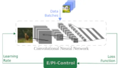
We consider a CNN as being our plant, and the data used in training are seen as a disturbance, see Figure 1.

Fig. 1: CNN control schema.

B. The disturbance: data batches

We consider a training dataset that consists of several data instances, such as images. And each data instance belongs to only one class c, where c ∈ {1, . . . , C}, representing for instance the main object on the picture. Data instances, structured in batches, are assumed to arrive sequentially to the learning system over time. We set that each batch consists of B data instances. One iteration on the whole batch is called an epoch, E epochs are run on each batch. When the data of the new batch arrives, we discard the previous data

and continue learning only on the new ones. This enables to reduce the storing space and processing time compared to keeping all the data. The control system sampling time is thus one epoch, while the disturbance time scale is the batches’ one.

C. Performance Metrics: accuracy and loss

Two signals can be used to evaluate a neural network performance: validation accuracy and loss function, both varying through epochs. Validation accuracy, computed on the test set, is the percentage of instances for which the predicted class matches the ground truth. Loss function also compares the model predictions with the ground truth, but includes the notion of confidence in the prediction through the use of a distance. Cross-entropy is one of the most used multiclass classification loss function, and is thus the one we selected to be our output signal. It is the sum of cross-entropy error between targets and the predicted values done on the test set. We define yi,c as being the ground truth, indicating

for each image i if it belongs to class c (yi,c = 1) or not

(yi,c = 0). ˆyi,c is the CNN output, indicating the predicted

probability of the image i to belong to class c. The loss function thus defined as follows:

loss = −1 T T X i=1 C X c=1

yi,clog(ˆyi,c) + (1 − yi,c)log(1 − ˆyi,c)

(1) with T the size of the test set. The lower the value of loss function, the better the model is for the data, and as the entropy can’t be negative, the target loss value is 0. Hence, the loss function is our error signal.

Validation accuracy is used as an a posteriori evaluation signal, as eventually, only the final prediction matters, what-ever its confidence. Swhat-everal metrics are extracted from the accuracy signal to reflect the CNN training performances. The end value of the accuracy is indeed the key factor. However, accuracy’s converging speed is also important engineering concern: for complex image datasets such as ImageNet, state of the art training strategies take up to a few days. Another important metric is the stability of the accuracy curve, especially for the epochs toward the end of the learning. A low standard deviation of the accuracy provides more guarantees on the final CNN performances. Eventually, the final value of the loss function is also of interest, as it allows to evaluate the model overfitting on data when compared to accuracy value.

D. The Control Signal: the learning rate

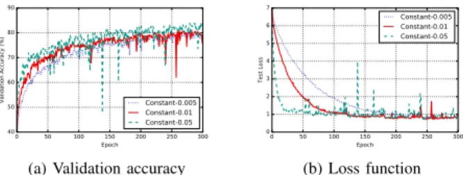
The learning rate λ is our control signal. To illustrate that the learning rate is a control signal for our online scenario, we study the impact of different constant learning rate on the variation of the accuracy and loss functions over epochs. Figure 2 is the application of three constant learning rates (λ ∈ {0.005, 0.01, 0.05}, corresponding to Bengio’s recom-mendation [5], larger and smaller) for training on CIFAR-10 dataset, with new data batches arriving every 60 epochs (see Section V-A for more details). The accuracy and loss

signals differ according to the learning rate (see Figure 2): with λ = 0.05, the accuracy improves the fastest and the loss also quickly converges to its lower limit. However, the noise of the curve at the last epochs is also higher than with the two other scenarios because a large learning rate oscillates around the minimum. When λ = 0.005, the accuracy increase is slower but the loss function varies more smoothly, the loss value rarely rises.

Thus, the learning rate is able to influence our performance indicators: it is suitable as a control signal.

(a) Validation accuracy (b) Loss function

Fig. 2: Impact of different constant learning rates on accuracy and loss (CIFAR-10).

III. MOTIVATION

The experiments shown in Figure 2 illustrate the advan-tages and drawbacks of large and small learning rates. A natural thought is to combine their benefits through learning rate scheduling: an initial phase with a large learning rate to quickly converge to a high-level accuracy, then a smaller value to smoothly approach the minimum and avoid the bumps on validation accuracy and loss. In the state of the art, there are some commonly used learning rate strategies that vary the learning rate through time. In the following of the paper, we will introduce two learning rate laws: (i) Keras-Time-Based-decay and (ii) Exponential-Sine-Wave-decay. They will later be used in Section V to compare with our proposed methods.

Keras-Time-Based-decay is a commonly and widely used learning rate strategy in Keras [17], which is a famous python deep learning library. The learning rate is computed as follow:

λ(k) = λ(k − 1)

1 + δk (2) where k is the number of epochs since the arrival of the last batch, k ∈ {1, . . . , E}. δ is a hyperparameter enabling to tune the steepness of the time decay. We set λ(0) = 0.01 and δ = 0.001 as suggested in [5].

The second common schedule is the exponential decay, it has been successfully used in neural network training. A good implementation is exponential decay sine wave learning rate schedule [10]. The original schedule is implemented to an offline setting, so to adapt this learning rate schedule into our online setting, we need to adjust their strategy to allow the learning rate decays to around 0 at the ending epochs of each batch. We will refer to this strategy as Exponential-Sine-Wave-decay. The adapted version is calculated as follow:

λ(k) = λ(0)e−αkE _(γsin(βk

2π) + e

−αk

E _{+ 0.5) (3)}

where k shares the same definition as in eq. (2). E is the training epochs per batch. α, β and γ are three hyperparam-eters. In order to have a same behavior as in [10] during our shorter E, we set α = 3, β = 6 and γ = 0.4. The constant 0.5 in the equation is important, it makes sure that λ(k) is strictly positive.

IV. PERFORMANCE-BASEDLEARNINGRATELAWS

In all the related work strategies, the learning rate is decreasing with time, in a predefined manner. The only differences between these strategies is that for some the learning rate decreases slowly in the beginning and faster in the end and for others is the opposite. We therefore introduce our control strategy where the learning rate is automatically computed based on the loss function (see Fig 1). Nevertheless, according to the definition of the loss function, the absolute loss value in itself does not give us much information since different size of training dataset can change the absolute loss value. Therefore, we normalize the value of loss(k) by loss(k = 0), where loss(k) represents the loss value at kthepoch since the arrival of the last batch. Subsequently, we try three different control laws for com-puting the learning rate λ: Proportional-Control (P-Control), Proportional Derivative-Control (PD-Control) and a Mixed Exponential PD-Control (E/PD-Control).

A. P-Control

In this case the learning rate depends proportionally on the loss value as follows:

λ(k) = KP

loss(k)

loss(0) (4) In general the value of loss(k)_loss(0) varies between 0 and 1. Indeed, as the loss function decreases thanks to the Stochastic Gradient Descent, we know that we are approaching the minimum of the loss function and therefore the learning rate should be decreased in order not to skip it. The choice of KP is important for the speed of convergence. Based on trial

and error tests, we make it equal to the same value as the empirical starting learning rate from [17]: λ(0) = KP =

0.01.

B. PD-Control

On one side, the hypothesis behind P-Control is that the loss is always decreasing; as we are getting closer to a minimum, the learning rate should slow down to better approach it. On the other side if the loss has decreased during last epoch we are in the good direction to find the minimum so we should reward last learning epoch by increasing the learning rate. This can be seen as adding an integral action to our controller. We express our PD-Control as follows:

λ(k) = KP

loss(k) loss(0) − KD

loss(k) − loss(k − 1) loss(0) (5) where KP = 0.01, and the integral parameter is empirically

chosen at 5 times λ(0), as we choose λ(0) = 0.01 , then KD = 0.05. As −(loss(k) − loss(k − 1)) could also be

negative, the integral part will introduce oscillations to the learning rate. In order to avoid that λ(k) becomes negative due to the integral part, the PD-Control is turned to a P-Control if λ(k) in PD-P-Control gets a negative value. Indeed, the P-Control will always return a positive value for the learning rate, as the loss function is by definition positive. C. E/PD-Control

This third control law tries to accelerate the convergence speed by exponentially increasing the learning rate at the beginning of learning a new batch, as the data are new so there are more informations to learn. We present a two phases algorithm to control the learning rate: (i) an initial Exponential growth followed by (ii) a PD-Control. During the exponential growth period, the learning rate is increased each time step by a factor 2 to quickly reach the minimum. This phase is stopped when the loss starts increasing, and the learning rate is afterwards ruled by the PD-Control law. The PD phase is initialized with the last value of the learning rate before loss growth. The PD parameters are set according to the behavior of the systems during the E-phase. The E/PD-Control law during one batch is summarized in Algorithm 1.

Algorithm 1 E/PD-Control

1: λ(0) = 0.01

2: k = 1

3: while loss(k) ≤ loss(k − 1) do

4: λ(k) = 2λ(k − 1) = 2k_λ(0) 5: k = k + 1 6: end while 7: λ(k + 1) = λ(k)/2 8: KP = λ(k)/2 9: KD= 5 × λ(0) 10: for i ∈ {k + 2, . . . , E} do 11: λ(k) = KP loss(k) loss(0) − KD loss(k) − loss(k − 1) loss(0) 12: end for

V. CONTROLLAWSEVALUATION

In this section, the P, PI and E/PI-Control laws are evalu-ated in comparison with the state of the art. The stability of the E/PI-Control law is highlighted, and its robustness with regards to its initial configuration is presented. First, details on the datasets, CNNs and evaluation indicators are given. A. Experimental setup

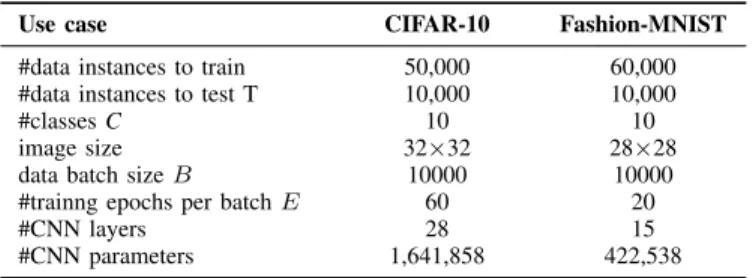
The controllers are evaluated on two datasets: CIFAR-10 and Fashion-MNIST. The CNN and scenario configurations for the two datasets is sum-up in Table I. As the images in CIFAR-10 have colors and are larger than the ones of Fashion-MNIST, a more complex CNN setting with more layers and parameters is used. Meanwhile, as there are more informations to extract from CIFAR-10, the number of epochs per batch is larger, allowing the accuracy curve to converge. All the values of hyperparameters of eq. (2)

and (3) we showed in section.III are tuned for CIFAR-10, as Fashion-MNIST has shorter epochs per batch, we will change δ to 0.01 of eq. (2), and set α = 2, β = 18 of eq. (3) for Fashion-MNIST experiment learning rate schedule.

To eliminate the influence of the CNN’s weights starting point to the final accuracy, we initialize the weights of each layer of CNN by Xavier uniform initializer [4], all the results will be averaged on 3 time experiment results. All code is implemented with Keras library [17].

TABLE I: CNN configuration

Use case CIFAR-10 Fashion-MNIST #data instances to train 50,000 60,000 #data instances to test T 10,000 10,000

#classes C 10 10

image size 32×32 28×28 data batch size B 10000 10000 #trainng epochs per batch E 60 20

#CNN layers 28 15

#CNN parameters 1,641,858 422,538

For performance evaluation, we measure several indicators on the accuracy and loss signals, the first one being their final value. To quantify the accuracy’s converging speed, we will report for each experiment the epoch at which they reached 95% of their final accuracy. To compare the influence of each learning rate strategy on stability of validation accuracy, we will also compare the standard deviation of the accuracy curve on the last 10% epochs of each experiment.

B. Stability analysis

Stability of the presented algorithms needs to be proved to ensure that the error signal (the loss function) will not diverge, and ideally converge to 0. The stability theory behind the algorithm is based on the SGD: the direction of the gradient is always set to decrease the loss. The only case that loss will increase is because the learning rate is too large (i.e. we skipped the minimum). The stability of the P and PD-Controllers are ensured via a proper parametrization of KP and KD. The E/PD-Control law allows the learning rate

to exponentially grow, however the learning rate is switched to a PD law as soon as the loss increases. The reset of the learning rate to the previously stable value (7th− 9th_{line of}

Algorithm 1) enables to properly initialize the PD. C. P, PD and E/PD-Control Performances Validation

The three control laws presented in Section IV are evalu-ated on CIFAR-10. Results are reported in Figure 3 through the accuracy 3a and loss functions 3b, and the corresponding control signals are illustrated in Figure 4, For the P and PD in 4a and for the E/PD law in 4b. There are few differ-ences between P and PD control performances, while the E/PD-Control is significantly faster (61 epochs rising time compared to 130 for the P and PD), converges to a higher accuracy (+7%) and lower loss (-37%) and the standard deviation of the accuracy at the end of the experiment is three times lower. We see from the first epochs that the E-phase

(a) Validation accuracy (b) Loss function

Fig. 3: Performances of state of the art, P, PD and E/PD-Control (CIFAR-10).

(a) P and PD-Control (b) E/PD-Control

Fig. 4: Control signal of state of the art, P, PD and E/PD-Control (CIFAR-10).

enables to properly tune the initial value of the PD, which then significantly increases the validation accuracy. The P and PD-Control learning rate signal (Figure 4a) illustrates that a reset of the learning rate at the arrival of a new batch is not necessary beneficial if the value is not carefully chosen, as for the E/PD-Control.

The loss function with the PD-Control declines a little bit faster than with the P-Control at beginning, and do not present a large peak around epoch 240. Those advantages made us opt for the PD-Control to combine with the initial E-phase.

D. Comparison with state of the art

Comparison of the state of the art learning rate strategies to our E/PD-Controller is provided for CIFAR-10 (Figures 3 and 4) and for Fashion-MNIST (see Figure 5 for the accuracy and loss and Figure 6 for the learning rate evolution through epochs).

E/PD-Control provides the best results for all the indica-tors for CIFAR-10. It converges faster and has a smallest standard deviation of last 10% epochs among all the strate-gies, it reaches at a higher final validation accuracy (+3%) and a lower loss. Keras-Time-Based-decay has a closer final accuracy and loss to E/PD-Control. But the deviation of its accuracy curve is bigger than E/PD-Control, especially at the beginning of learning a new batch.

Regarding Fashion-MNIST dataset, results are similarly in favor of the E/PD-Controller, even if the differences are smaller. As this dataset is easier than CIFAR-10, all strategies reached a high validation accuracy and lower loss, the standard deviation of accuracy of last 10% epochs is also very small.

(a) Validation accuracy (b) Loss function

Fig. 5: Performances of state of the art and E/PD-Control on Fashion-MNIST.

(a) State of the art strategies (b) E/PD-Control

Fig. 6: Control signal for the state of the art and E/PD-Control on Fashion-MNIST.

E. Robustness to initial value of the learning rate

The E/PD-Control is now compared with the best strategy from the state of the art (Keras-Time-Based-decay) when the initial learning rate varies. Results are showed in Table II for CIFAR-10 and Table III for Fashion-MNIST.

Among all the experiments on CIFAR-10, there are only one case for which Keras-Time-Based-decay law has a better indicator (final validation accuracy at initial learning rate 0.05). The difference is very small, and standard deviation of the indicator itself is large. Moreover, if we check the accuracy’s standard deviation during the last 10% epochs, Keras-Time-Based-decay still has a strong oscillation, which makes the model unpredictable. E/PD-Control also shows the advantage on converging time, it makes the model converge faster and rarely affected by the initial values.

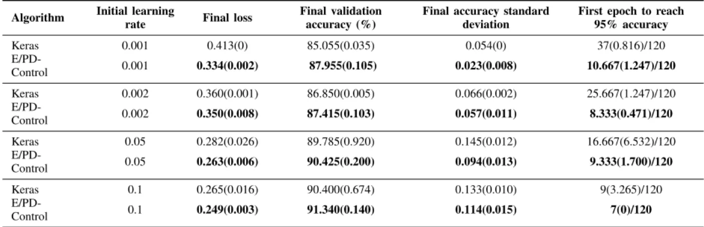
Table III shows the robustness results on Fashion-MNIST. E/PD-Control still shows a fast converging speed, reaching 95% of final accuracy just using 7 to 10 epochs. The perfor-mances for the final loss and accuracy final standard devi-ation are similar for the two strategies. The E/PD-Control’s final accuracy performances among all the experiments is more stable than with Keras-Time-Based-decay, which again, shows that E/PD-Control is more robust to the initial learning rate variations.

VI. CONCLUSION

When performing image classification tasks with neural networks, often comes the issue of on-line training, from sequential batches of data. Iterative training of CNNs is driven by a learning rate - how much to update the network weights with the new data - which value is usually ruled by a time decreasing function. This paper presents a control approach to the challenge of on-line training of CNNs, that

TABLE II: Robustness experiments with varying initial learning rate on CIFAR-10. Mean value (and standard deviation) over 3 runs. The best results are highlighted in bold.

Algorithm Initial learning

rate Final loss

Final validation accuracy (%)

Final accuracy standard deviation

First epoch to reach 95% accuracy Keras 0.001 0.849(0.023) 79.075(0.485) 0.371(0.053) 161.333(24.495)/300 E/PD-Control 0.001 0.648(0.015) 82.035(0.465) 0.057(0.013) 61.333(0.471)/300 Keras 0.002 0.745(0.026) 80.180(0.445) 0.415(0.049) 118.333(9.78)/300 E/PD-Control 0.002 0.586(0.006) 83.150(0.225) 0.077(0.017) 62(0)/300 Keras 0.05 0.727(0.006) 85.640(0.523) 1.630(0.085) 103.333(2.859)/300 E/PD-Control 0.05 0.555(0.005) 85.060(0.090) 0.117(0.001) 61.333(0.471)/300 Keras 0.1 0.829(0.180) 84.433(2.82) 1.609(0.432) 77.333(32.785)/300 E/PD-Control 0.1 0.578(0.013) 85.075(0.585) 0.345(0.16) 65(0.816)/300

TABLE III: Robustness experiments with varying initial learning rate on Fashion-MNIST. Mean value (and standard deviation) over 3 runs. The best results are highlighted in bold.

Algorithm Initial learning

rate Final loss

Final validation accuracy (%)

Final accuracy standard deviation

First epoch to reach 95% accuracy Keras 0.001 0.413(0) 85.055(0.035) 0.054(0) 37(0.816)/120 E/PD-Control 0.001 0.334(0.002) 87.955(0.105) 0.023(0.008) 10.667(1.247)/120 Keras 0.002 0.360(0.001) 86.850(0.005) 0.066(0.002) 25.667(1.247)/120 E/PD-Control 0.002 0.350(0.008) 87.415(0.103) 0.057(0.011) 8.333(0.471)/120 Keras 0.05 0.282(0.026) 89.785(0.920) 0.145(0.012) 16.667(6.532)/120 E/PD-Control 0.05 0.263(0.006) 90.425(0.200) 0.094(0.013) 9.333(1.700)/120 Keras 0.1 0.265(0.016) 90.400(0.674) 0.133(0.010) 9(3.265)/120 E/PD-Control 0.1 0.249(0.003) 91.340(0.140) 0.114(0.015) 7(0)/120

decides the learning rate value based on the expected learning need (i.e. the CNN loss function) instead of being time-based. E/PD-Control is a strategy that combines a phase of exponential growth of the control signal (i.e. learning rate) with a PD controller, which parameters are automatically adapted based on the E-phase.

Stability of the control strategy is provided, and evaluation highlights that E/PD-Control achieves a higher accuracy level in a shorter time than the state of the art solutions. Robustness of the approach is illustrated by its performances on two different datasets, and enforced by a sensitivity analysis regarding its initialization.

This work could be further extended by the addition of a triggering mechanism to smartly adapt the number of epochs needed at each batch processing. Moreover, we want to investigate the performances of the E/PD-Control in the scenario when new classes appear in some batches.

REFERENCES

[1] Y. LeCun et al., “Lenet-5, convolutional neural networks,” URL: http://yann.lecun.com/exdb/lenet, p. 20, 2015.

[2] B. T. Morris and M. M. Trivedi, “Learning, modeling, and classifica-tion of vehicle track patterns from live video,” IEEE Transacclassifica-tions on

Intelligent Transportation Systems, vol. 9, no. 3, pp. 425–437, Sep. 2008.

[3] M. Lease, “On quality control and machine learning in crowdsourc-ing,” in Human Computation, vol. 11, no. 11, 2011.

[4] X. Glorot and Y. Bengio, “Understanding the difficulty of training deep feedforward neural networks,” in Proceedings of the Thirteenth International Conference on Artificial Intelligence and Statistics, AIS-TATS 2010, Chia Laguna Resort, Sardinia, Italy, May 13-15, 2010, pp. 249–256.

[5] Y. Bengio, “Practical recommendations for gradient-based training of deep architectures,” in Neural networks: Tricks of the trade. Springer, 2012, pp. 437–478.

[6] S. Ioffe and C. Szegedy, “Batch normalization: Accelerating deep network training by reducing internal covariate shift,” CoRR, vol. abs/1502.03167, 2015. [Online]. Available: http://arxiv.org/abs/1502.03167

[7] L. N. Smith, “Cyclical learning rates for training neural networks,” in Applications of Computer Vision (WACV), 2017 IEEE Winter Conference on. IEEE, 2017, pp. 464–472.

[8] S. Ruder, “An overview of gradient descent optimization algorithms,” arXiv preprint arXiv:1609.04747, 2016.

[9] X. Wu, R. Ward, and L. Bottou, “Wngrad: Learn the learning rate in gradient descent,” arXiv preprint arXiv:1803.02865, 2018.

[10] W. An, H. Wang, Y. Zhang, and Q. Dai, “Exponential decay sine wave learning rate for fast deep neural network training,” in 2017 IEEE Visual Communications and Image Processing (VCIP), Dec 2017, pp. 1–4.

[11] A. Krizhevsky and G. Hinton, “Learning multiple layers of features from tiny images,” Master’s thesis, Department of Computer Science, University of Toronto, 2009.

[12] H. Xiao, K. Rasul, and R. Vollgraf, “Fashion-mnist: a novel image dataset for benchmarking machine learning algorithms,” arXiv preprint arXiv:1708.07747, 2017.

[13] K. He, X. Zhang, S. Ren, and J. Sun, “Deep residual learning for image recognition,” 2016 IEEE Conference on Computer Vision and Pattern Recognition (CVPR), pp. 770–778, 2016.

[14] R. Yamashita, M. Nishio, R. K. G. Do, and K. Togashi, “Convolutional neural networks: an overview and application in radiology,” Insights into Imaging, vol. 9, no. 4, pp. 611–629, Aug 2018.

[15] D. H. Hubel and T. N. Wiesel, “Receptive fields and functional architecture of monkey striate cortex,” Journal of Physiology (London), vol. 195, pp. 215–243, 1968.

[16] K. Fukushima, “Neocognitron: A self-organizing neural network model for a mechanism of pattern recognition unaffected by shift in position,” Biological Cybernetics, vol. 36, pp. 193–202, 1980. [17] F. Chollet et al., “Keras,” https://github.com/fchollet/keras, 2015.