Clinical event prediction and understanding with deep neural networks

Clinical Event Prediction and Understanding

Deep Neural Networks

DeepNeual etwrksOF MASSACHUSETS TECHNOLOGYINSTITUTE

by

AUG 14 2017

Harini Suresh

_LIBRARIES

Submitted to the Department of Electrical Engineering and Computer

ARCHIVES

Science

in partial fulfillment of the requirements for the degree of

Master of Engineering in Computer Science and Engineering

at the

MASSACHUSETTS INSTITUTE OF TECHNOLOGY

May 2017

? on3

@

Harini Suresh. All rights reserved.

The author hereby grants to MIT permission to reproduce and to

distribute publicly paper and electronic copies of this thesis document

in whole or in part in any medium now known or hereafter created.

Author

Signature redacted

Department of Electrical Engineering and Computer Science

Certified by

Accepted by

Signature redacted

May 26, 2017

Peter Szolovits

Professor of Electrical Engineering and Computer Science

Thesis Supervisor

Signature redacted

Christopher J. Terman

Chairman, Master of Engineering Thesis Committee

Clinical Event Prediction and Understanding with

Deep Neural Networks

by Harini Suresh

Submitted to the Department of Electrical Engineering and Computer Science in Partial Fulfillment of the Requirements for the Degree of

Master of Engineering in Electrical Engineering and Computer Science

Abstract

Real-time prediction of clinical interventions remains a challenge within intensive care units (ICUs). This task is complicated by data sources that are noisy, sparse, heterogeneous and outcomes that are imbalanced. In this thesis, we integrate data from all available ICU sources (vitals, labs, notes, demographics) and focus on learn-ing rich representations of this data to predict onset and weanlearn-ing of multiple invasive interventions. We first investigate the ability of both deep and sequence autoencoders to effectively learn low-dimensional and dense underlying patient states in an unsu-pervised way. In addition, we compare these representations along with both long short-term memory networks (LSTM) and convolutional neural networks (CNN) for prediction of five intervention tasks: invasive ventilation, non-invasive ventilation, vasopressors, colloid boluses, and crystalloid boluses. Our predictions are done in a forward-facing manner to enable "real-time" performance, and predictions are made with a six hour gap time to support clinically actionable planning. We achieve state-of-the-art results on our predictive tasks using deep architectures. We explore the use of feature occlusion to interpret LSTM models, and compare this to the inter-pretability gained from examining inputs that maximally activate CNN outputs. We show that our models are able to significantly outperform baselines in intervention prediction, as well as provide insight into model learning, which is crucial for the adoption of such models in practice.

Acknowledgments

I would like to thank my advisor, Peter Szolovits, for his consistent guidance and

reassurance. Whenever I was frazzled, Pete was calm, and in turn helped me believe in my own ability to solve problems. He allowed this work to be my own while always asking the right questions to help me expand my mindset and do better research.

I would also like to thank another mentor in my lab, Marzyeh Ghassemi. Between

brainstorming sessions, technical guidance, life advice, daily motivation, and constant support, she made the past year both rewarding and enjoyable.

I am extremely grateful to my colleagues and labmates, Tristan, Wille, Matt, Nathan and Jen. They have continually helped me by collaborating on research, being a sounding board for ideas, editing papers and always being supportive. My sincere thanks also goes to our collaborators Alistair Johnson and Leo Celi for providing their expertise and input.

Last but not least, I would like to thank my parents for always encouraging me to pursue my goals without inhibition. Their continued support has made the past 22 years fantastic, and I would most definitely not be here without them.

Contents

1 Introduction 11

2 Background 17

2.1 Long Short-Term Memory Networks . . . . 17

2.2 Convolutional Neural Networks . . . . 18

3 Related Work 21 3.1 Computational Phenotyping . . . . 21

3.2 Actionable Prediction Tasks . . . . 22

4 Data 25 4.1 MIMIC Database . . . . 25

4.2 Types of Data Used . . . . 25

4.3 Data Processing . . . . 28

5 Unsupervised Patient Phenotyping 29 5.1 M ethods . . . . 29 5.1.1 Features . . . . 29 5.1.2 Autoencoders . . . . 30 5.1.3 Experimental Settings . . . . 30 5.2 R esults . . . . 32 5.2.1 Reconstruction Performance . . . . 32 5.2.2 Predictive Ability . . . . 34 5

6 Actionable Intervention Prediction 35

6.1 Data Representation . . . . 35

6.2 Prediction Task . . . . 36

6.3 M ethods . . . . 37

6.3.1 Long Short-Term Memory Network (LSTM) . . . . 37

6.3.2 Convolution Neural Network (CNN) . . . . 38

6.3.3 Autoencoder Representations . . . . 38

6.3.4 Experimental Settings . . . . 39

6.3.5 Evaluation . . . . 39

6.3.6 Interpretibility . . . . 40

6.4 R esults . . . . 41

6.4.1 Physiological Words Improve Predictive Task Performance With High Class Imbalance . . . . 41

6.4.2 Feature-Level Occlusions Identify Important Per-Class Features 41 6.4.3 Convolutional Filters Target Short-term Trajectories . . . . . 43

6.4.4 Supervised Representations Outperform Unsupervised . . . . . 46

7 Conclusion 47 A Tables 49 A.1 Generated Topics . . . . 49

6

List of Figures

4-1 Data preprocessing and feature extraction with numerical measure-ments and lab values, clinical notes and static demographics. . . . . . 27

5-1 Schematics of autoencoder architectures. . . . . 31

5-2 Schematics of LSTM and CNN model architectures. . . . . 32

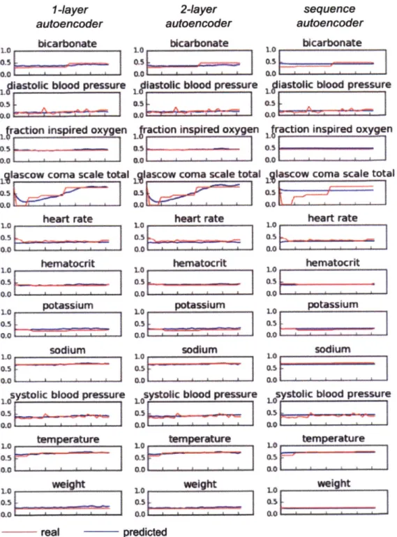
5-3 Examples of feature reconstructions for a single patient for an interval

of 32 hours. Note that the scales for each variable are normalized between 0 and 1 based on the population minimum and maximum.

All autoencoders are able to predict the values of variables well, and

the sequence autoencoder generally produces a smoother trajectory. 33

6-1 Converting data from continuous timeseries format to discrete "phys-iological words." The numeric values are first z-scored and rounded, and then each z-score is made into its own category. On the right, glucose_-2 indicates the presence of a glucose value that was 2 stan-dard deviations below the mean. A row containing all zeros for a given variable indicates that the value for that variable was missing at the tim estep . . . . 36 6-2 Given data from a fixed-length (6 hour) sliding window, models predict

the status of intervention in a prediction window (4 hours) after a gap time (6 hours). Windows slide along the entire patient record, creating multiple examples from each record. . . . . 37 6-3 Schematics of LSTM and CNN model architectures. . . . . 38

6-4 We are able to make interpretable predictions using the LSTM and oc-cluding specific features. The top eight features that cause a decrease in prediction AUC for each intervention task. In general, physiologi-cal data were more important for the more invasive interventions mechanical ventilation (6-4a, 6-4b) and vasopressors (6-4c, 6-4d) while clinical note topics were more important for less invasive tasks

- non-invasive ventilation (6-4e, 6-4f) and fluid boluses (6-4g, 6-4h). Note that all weaning tasks except for ventilation have significantly less AUC variance. . . . . 42

6-5 Trajectories of the 10 maximally and minimally activating examples

for onset of each of the interventions. . . . . 44

6-6 Trajectories generated by adjusting inputs to maximally activate a

specific output node of the CNN. . . . . 45

List of Tables

4.1 V ariables . . . . 26

4.2 Dataset Statistics . . . . 27 6.1 The proportion of each intervention class. Note that colloid and

crys-talloid boluses are not administered for specific durations, and thus have only a single class (onset). NI = non-invasive. . . . . 37 6.2 Comparison of model performance on five targeted interventions.

Mod-els that perform best for a given (intervention, task) pair are bolded. 45

A. 1 Most probable words in the topics most important for intervention

predictions. . . . . 50

Chapter 1

Introduction

As Intensive Care Units (ICUs) play an increasing role in acute healthcare delivery

[59], clinicians must anticipate patient care needs in a fast-paced, data-overloaded setting. The secondary analysis of healthcare data is a critical step toward improving modern healthcare, as it affords the study of care in real care settings and patient populations [161.

Prognostic models to predict the outcome of patients in Intensive Care Units

(ICU)

are valuable for many reasons, among them:

1. Risk stratification: Stratifying patients by their risk to various adverse events

provides a way to evaluate and compare ICUs and new therapies. For example, if one hospital has a higher mortality rate than another, it does not necessarily mean that the hospital is performing more poorly. It may just be a reflection of a difference in the average health of the two different patient populations. The ability to empirically risk stratify patients essentially allows these evaluations to calibrate themselves to the unique state of patients in the hospital for more accurate comparisons [55].

2. Resource utilization: The ICU is a high-cost and resource-constrained envi-ronment. ICUs are already over-crowded, and many patients are not able to receive critical care that would be beneficial to them [341. In this environment, utilization strategies are clearly essential. Detsky et al. showed that both total

expenditure and expenditure per day in the ICU were highest for patients whose outcomes were the most unexpected when compared to a physician's predicted prognosis [17]. Being able to predict how at-risk various patients are throughout their stay provides an empirical basis for scheduling and resource allocation. It also provide estimates for how long a patient should continue a therapy or what the optimal time for discharging a patient is [37].

3. Clinical decision-making: Predictive models can provide a reliable and unbiased

way to use past experiences to guide future ones. Outside of reducing expendi-tures [171, this guidance can lead to more efficient and helpful care for patients

[26]. Physicians perform clinical decision-making everyday. However, a

data-derived prognostic model provides the advantage of being supported by more data than any one physician's experiences, and thus being less biased than any single doctor. When implemented effectively, prognostic models have improved patient care. For example, the Thrombolytic Predictive Instrument (TPI) esti-mates the risk of key outcomes of thrombolytic therapy. Sekler et al. performed a randomized controlled clinical effectiveness trial and showed that printing the TPI on electrocardiogram headers improved and expedited the appropriate use of therapies for patients [54].

Throughout this thesis, we focus specifically on clinical decision-making. Elec-tronic Healthcare Record (EHR) systems that meet federal requirements are present in most acute care hospitals (97% in 2014 [6]) and office-based physicians' prac-tices (78% in 2015 [32]). This widespread availability allows new investigations into evidence-based decision support.

Specifically, we aim to predict when patients need or can be weaned off of certain interventions. This is important because the efficacy of interventions can drastically vary from patient to patient, and unnecessarily administering an intervention can be harmful and expensive [19].

Understanding how patients react to interventions and progress through time de-pends on a robust understanding of the patient's underlying acuity

[7].

Traditional

measures of acuity are often based on mortality evaluated at a single endpoint [5, 23], or on static scores such as SAPS that don't take into account evolving clinical infor-mation [48, 1.

We aim to create richer representations of patient health with the end goal of predicting actionable interventions. A model of patient health that is able to capture complex relationships in physiological signals over time is key to accurately predict-ing onset/weanpredict-ing of interventions for different patients and necessary for successful personalized medicine. Continuous, forward-facing event prediction is particularly applicable in an ICU setting, where we want to account for evolving clinical needs

and information throughout the patient's stay.

This type of patient phenotyping is challenging because robust representations of human physiology are complicated, and contain many non-obvious dependencies between observed measurements. Moreover, modeling evolving clinical information requires using timeseries data, but this data is often varying-length, irregularly sam-pled or has missing values. Previously, multitask gaussian processes have been tested for modelling patient acuity but only in Traumatic Brain Injury (TBI) patients [24] or only using longitudinal billing data [7].

To this end, we first experiment with using autoencoders for physiological time-series signal reconstruction. Autoencoders are neural networks where the target values are the same as the input values, and the hidden layer(s) compress the inputs into a lower dimensional embedding. Since this embedding tries to reconstruct the original input, it must capture fundamental features about the input timeseries, and can be thought of as encoding an underlying patient representation. Feature learning in this approach is entirely unsupervised, so unlike traditional acuity measures it is not lim-ited by a manually-defined feature space. Furthermore, recurrent autoencoders are able to model signals of varying length and are robust to missing data due to the ability of Long-Short Term Memory (LSTM) cells to forget unimportant inputs.

Furthermore, we focus on actionable insights using robust patient representations

by predicting onset and weaning of interventions. Any treatments come with inherent

risks, and we target interventions that span a wide severity of needs in critical care

- specifically, invasive ventilation, non-invasive ventilation, vasopressors, colloid bo-luses, and crystalloid boluses. Mechanical ventilation is commonly used for breathing assistance, but has many potential complications [63] and small changes in ventilation settings can have large impact in patient outcomes [58]. Vasopressors are a common

ICU medication, but there is no robust evidence of improved outcomes from their use

[47], and some evidence they may be harmful [19]. Fluid boluses are used to improve

cardiovascular function and organ perfusion. There are two bolus types: crystalloid and colloid. Both are often considered as less aggressive alternatives to vasopressors, but there are no multi-center trials studying whether fluid bolus therapy should be given to critically ill patients, only studies trying to distinguish which type of fluid should be given [43].

Capturing the complex relationships across many disparate data types is key for predictive performance in our tasks. We take advantage of the success of deep learn-ing models to capture rich representations of data with little hand-engineerlearn-ing by domain experts. We use long short-term memory networks (LSTM)

[311,

which have been shown to effectively model complicated dependencies in timeseries data

[3].

Pre-viously, LSTMs have achieved state-of-the-art results in many different applications, such as machine translation [28], dialogue systems [121 and image captioning [61]. They are well-suited to our modeling tasks because clinical conditions may be spread over several hours. We compare the LSTM models to a convolutional neural network

(CNN) architecture that has previously been explored for longitudinal laboratory

data [521. All models predict outcomes in a continuous manner given any patient record over vitals, labs, demographic, and notes. In doing so, we:

1. Achieve state-of-the-art prediction results in our forward-facing, hourly

predic-tion of clinical intervenpredic-tions (onset, weaning, and continuity) that could be used at the time of care.

2. Demonstrate that different data modalities and features are most important for different types of predictive tasks in our LSTM using feature occlusion. This is an important step in making models more interpretable by physicians.

14

3. Highlight patient trajectories that lead to the most and least confident

pre-dictions in our CNN across outcomes and features, further aiding model inter-pretability.

4. Compare supervised and unsupervised patient representations in their ability to predict onset and weaning of interventions.

Chapter 2

Background

2.1

Long Short-Term Memory Networks

Long Short Term Memory Networks (LSTMs)

[311

are a variant of Recurrent Neural Networks (RNNs) in which each hidden unit contains several logic gates that allow it to forget specific information from a certain timestep, or allow information to pass through several timesteps unchanged.

While traditional RNNs suffer from the vanishing gradient problem that arises when backpropagating gradients to timesteps far in the past [291, the gated flow of information in LSTMs avoids this training pitfall [30]. LSTM cells are thus able to effectively model varying-length data and capture long-term dependencies [13].

LSTMs have achieved state-of-the-art results in many different applications, such as machine translation [11], dialogue systems [12], and image captioning [13].

Having seen the input sequence x, ... xt of a given example, an LSTM performing

classification predicts #t, a probability distribution over the outcomes, with target outcome yt:

hi ... ht = LSTM(x1. ... xt) (2.1)

= softmax(Wyht + by) (2.2)

where xi E RX, Wv E RNcxL2, ht

C

RL2, by G R Nc where V is the dimensionality of

the input (number of variables), N0 is the number of classes we predict, and L2 is

the second hidden layer size.

LSTM performs the following update equations for a single layer, given its

previ-ous hidden state and the new input:

ft = U(Wf[htl1, xt] + bf) (2.3)

it= o-(Wi[ht-I, xt] + bi) (2.4)

it = tanh(We[ht_ 1, xt] + b,) (2.5)

ct = ft 0 ct_1 + it it (2.6)

ot = U(WO[ht-1, xt] + bo) (2.7)

ht = ot 0 tanh(ct) (2.8)

where Wf, W, Wc, W, E RLIx(Li+V)I bf, b b, bo E RL1 are learned parameters, and

ft, it Ii, t , ot, ht E RL1. In these equations, -stands for an element-wise application of

the sigmoid (logistic) function, and 0 is an element-wise product. This is generalized to multiple layers by providing ht from the previous layer in place of the input.

2.2

Convolutional Neural Networks

In a Convolutional Neural Network (CNN) [401, a number of filters (or kernels) slide across an image to produce a convolved output. Convolutional layers are usually alternated with max-pooling layers that achieve non-linear down-sampling, and fol-lowed by fully connected layers at the end of the network to produce a classification output.

CNNs have achieved state-of-the-art results in video classification

[36],

image recognition [56], image segmentation

[42],

and transfer learning for image process-ing tasks [49].

They have also been extended successfully to the ID space for timeseries classifi-cation. In this case, the convolutional kernels are one-dimensional and operate along the temporal dimension

[65].

CNNs have proven to be useful for timeseries because

important factors may often operate at different and unpredicatable timescales. For example, for sepsis prediction, certain fluctuation patterns in body temperature that occur over several hours have high predictive value

[181.

It is unlikely that pre-defined features will capture the most predictive variations at all important timescales.

To this end, CNNs have been used for human activity recognition using sensor-based timeseries data

[62],

for seizure prediction from intracranial EEG signals

[46],

as well as evaluated on several tasks from the UCR timeseries classification archive [14].

Chapter 3

Related Work

3.1

Computational Phenotyping

Clinical data is noisy, sparse, and heterogeneous. Additionally, many different pat-terns present both across features and time can be very important. Therefore, raw data often benefits from being transformed into a more dense and semantically mean-ingful feature space that captures the important facets of the data. Furthermore, following this transformation, patient representations can be examined or clustered to extract meaningful descriptors of health [351.

One way to create such a representation of patient state is by using features pre-defined by an expert (i.e. a physician) . However, this approach can be costly, time-consuming and/or miss important factors. Discovering latent representations automatically is a more sustainable approach and is more likely to create optimal representations [9]. When inferring latent representations, unsupervised methods have the advantage of identifying patterns that completely represent the source data, without the risk of overfitting to any specific prediction task [39].

In this vein, Multitask Gaussian Processes

[24]

were used to model multivariate clinical timeseries by transforming the irregularly-sampled data into a new discrete latent space. The inferred representations were then assessed in their ability to predict patient acuity. When used as additional classification features, these representations improved predictive performance.

Autoencoders have been trained on random 30-day patches of serum uric acid measurements

[39]

to display learned population subtypes, though using these features did not significantly improve performance on a supervised classification task.

Stacked denoising autoencoders were trained on aggregated event data [45] to learn underlying patient phenotypes. The learned features improved performance when predicting a subset of future ICD-9 codes.

These approaches concatenate or aggregate timestamped data, which makes tem-poral trends difficult to capture. Rather, it may be advantageous to use a sequence-modeling approach to capture time-dependencies in the data. We make use of se-quence autoencoders for this purpose.

Sequence autoencoders take in measured signals one timestep at a time into a layer of LSTM (Long-Short Term Memory) cells and produce a fixed-length embedding. This embedding is then used as input to another layer of LSTM cells that try to predict the original input sequence.

Sequence autoencoders using LSTM cells were inspired by the success of general sequence-to-sequence models applied to machine translation. They were recently used as an initialization step for recurrent neural networks for text classification [15], but have not been applied to the clinical space.

3.2

Actionable Prediction Tasks

Clinical decision-making often happens in settings of limited knowledge and high uncertainty; for example, 55 of the 72 ICU interventions evaluated in randomized controlled trials (RCTs) resulted in non-significant results [501. The goal of post-hoc EHR analysis is to gain insight from healthcare data previously collected during patient care.

Recent studies have applied recurrent neural networks (RNNs) to modeling se-quential EHR data to tag ICU signals with billing code labels [8, 41, 10] or to identify the impact of different drugs for diabetes

[38].

Razavian et. al. [52] compared CNNs to LSTMs for longitudinal outcome prediction on billing codes using lab tests.

22

. ... n"'

Although predicting billing codes may be useful for automating some billing tasks, the clinical usefulness of this prediction as well as the predictive strength of these models (many billing codes may be indicating chronic diseases, rather than disease onset) is unclear.

Others have focused on using representations of clinical notes [23] or patient phys-iological signals to predict mortality [24]. Evaluating mortality at a single endpoint, while providing a proxy for patient acuity, may not provide enough information to be clinically useful and actionable.

Previous work that has targeted on interventions in ICU populations have often either focused on a single outcome or used data from specialized cohorts. Such mod-els with vasopressors as a predictive target have achieved AUCs of 0.79 in patients receiving fluid resuscitation [22], 0.85 in septic shock patients [53], and 0.88 for onset after a 4 hour gap and 0.71 for weaning, only trained on patients who did receive a vasopressor

[60].

However, we train our models on general ICU populations in order to make them more applicable. In the most recent prior work on interventions, also on a general ICU population, the best AUC performances were 0.67 (ventilation),

0.78 (vasopressor) for vasopressor onset prediction after a 4 hour gap [25]. These

were lowered to 0.66 and 0.74 with a longer gap time of 8 hours.

With regard to interpretability, Choi et. al. [11] used temporal attention to identify important features in early diagnostic prediction of chronic diseases from time-ordered billing codes.

24

Chapter 4

Data

4.1

MIMIC Database

We use data from the Multiparameter Intelligent Monitoring in Intensive Care

(MIMIC-III v1.4) database [33]. Since 2001, the MIMIC database has been built up and

main-tained by the Laboratory of Computational Physiology at the Massachusetts Institute of Technology, Beth Israel Deaconess Medical Center, and Philips Healthcare, with support from the National Institute of Biomedical Imaging and Bioinformatics [23].

The most recent version of this database, MIMIC III, contains data from around

38,600 adults, comprising over 58,000 hospital admissions, from 2001-2012.

The data includes features such as demographics, bedside vital sign measurements, laboratory test results, procedures, medications, caregiver notes, imaging reports, and mortality (both in and out of hospital). MIMIC is unique in its scale, as well as the robustness of the included variables and presence of highly granular data.

4.2

Types of Data Used

We consider patients 15 and older who had ICU stays from 12 to 240 hours and consider each patient's first ICU stay only. This yields 34,148 unique ICU stays. We use patients from the Medical Care Unit (MICU), Cardiac Care Unit (CCU),

Cardiovascular Intensive Care Unit (CVICU), Medical/Surgical Intensive Care Unit

(MSICU), Surgical Intensive Care Unit (SICU), and Trauma Surgical Intensive Care Unit (TSICU).

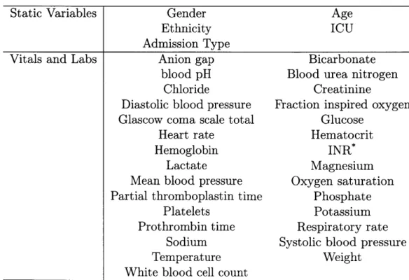
For each patient, we extract:

1. 5 static variables such as gender and age.

2. 29 time-varying vitals and labs such as oxygen saturation and blood urea nitro-gen. We use these 29 variables because they are the least sparse in the dataset, and have verified item IDs.

3. All available, de-identified clinical notes for each patient as timeseries across

their entire stay.

See Table 4.1 for a full list of static, vitals, and labs, and Table 4.2 for dataset statistics.

Table 4.1: Variables

Static Variables Gender Age

Ethnicity ICU

Admission Type

Vitals and Labs Anion gap Bicarbonate

blood pH Blood urea nitrogen

Chloride Creatinine

Diastolic blood pressure Fraction inspired oxygen

Glascow coma scale total Glucose

Heart rate Hematocrit

Hemoglobin INR*

Lactate Magnesium

Mean blood pressure Oxygen saturation Partial thromboplastin time Phosphate

Platelets Potassium

Prothrombin time Respiratory rate

Sodium Systolic blood pressure

Temperature Weight

White blood cell count International normalized ratio of the prothrombin time

variables

3 1 402

- Extract as hourly

~ x . timeselas

L ifor

Ktopc,D domw h6N wo rdorh.Ni I

A0:par" fr Dkhude 0-or

-0,-Dre:to*ldist. for docusrtd

________________ sa -Dir(i): vxrd dimtfor topich kE Or

__________________Unsupavisad LDA modal t lraermto

twforat*o

Replicate acros time F"

Figure 4-i: Data preprocessing and feature extraction with numerical and lab values, clinical notes and static demographics.

measurements

Table 4.2: Dataset Statistics

Train Test Patients Notes Elective Admission Urgent Admission Emergency Admission Mean Age Black/African American Hispanic/Latino White

CCU (coronary care unit)

CSRU (cardiac surgery recovery)

MICU (medical ICU) SICU (surgical ICU)

TSICU (trauma SICU)

Female Male ICU Mortalities In-hospital Mortalities 30 Day Mortalities 90 Day Mortalities Vasopressor Usage Ventilator Usage 27,318 564,652 4,536 746 22,036 63.9 1,921 702 19,424 4,156 5,625 9,580 4,384 3,573 11,918 15,400 1,741 2,569 2,605 2,835 8,347 11,096 27 6,830 140,089 1,158 188 5,484 64.1 512 166 4,786 993 1,408 2,494 1,074 861 2,924 3,906 439 642 656 722 2,069 2,732 Total 34,148 703,877 5,694 934 27,520 63.9 2,433 868 24,210 5,149 7,033 12,074 5,458 4,434 14,842 19,306 2,180 3,211 3,216 3,557 10,416 13,828 'I

4.3

Data Processing

Static variables were replicated across all timesteps for each patient. Vital and lab measurements are given timestamps that are rounded to the nearest hour. If an hour has multiple measurements for a signal, those measurements are averaged.

Clinical narrative notes were processed to create a 50-dimensional vector of topic proportions for each note using Latent Dirichlet Allocation [4, 27]. These vectors are replicated forward and aggregated through time [23]. For example, if a patient had a note A recorded at hour 3 and a note B at hour 7, hours 3-6 would contain the topic distribution from A, while hours 7 onward would contain the aggregated topic distribution from A and B combined. See Figure 4-1 for a schematic of data extraction and processing. Important topics are displayed in the Appendix.

Chapter 5

Unsupervised Patient Phenotyping

We use autoencoders to create low-dimensional embeddings of underlying patient phenotypes that we hypothesize are a governing factor in determining how different patients will react to different interventions. We compare the reconstruction perfor-mance of autoencoders that take fixed length sequences of concatenated timesteps as input with a recurrent sequence-to-sequence autoencoder. We evaluate our meth-ods on around 35,500 patients from the latest MIMIC III dataset from Beth Israel Deaconess Hospital.

5.1

Methods

5.1.1

Features

In this section, we use 29 vitals and labs from MIMIC III for each patient as hourly timeseries spanning their entire stay. These features were chosen because they were the least sparse, and had verified item IDs. A more detailed description of this data and preprocessing is found in Chapter 4.

Since there are many missing values, we first forward-fill for each patient using existing values, and then fill in remaining missing values with the mean value for that variable across all patients.

The work in this chapter was submitted to the NIPS 2016 Machine Learning for Healthcare workshop with Marzyeh Ghassemi.

We take one interval from each patient's record, resulting in 34,469 total examples. The data is split into training/validation/testing sets with a 70/10/20 split, stratified on in-hospital mortality in order to have a spectrum of patient severity in both the train and test sets.

5.1.2

Autoencoders

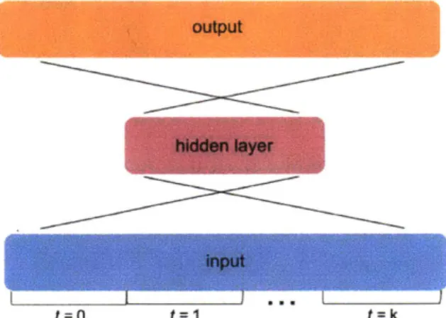
We test the ability of a simple autoencoder with a single hidden layer, an autoencoder with two hidden layers, and a sequence autoencoder to reconstruct the input (Figure

5-1). We also compare the performance of these models over inputs of different interval

lengths, specifically 4, 16, 32 and 64 hours.

For the fixed-length input autoencoders, we concatenate all 30 features for each hour throughout the given interval length. We use an embedding size equal to the total number of input values divided by 10 to achieve a compression factor of 10x.

The sequence autoencoder consists of a single hidden layer made up of LSTM cells. We feed in the input one timestep at a time. If we have k timesteps and f features per timestep, the hidden layer is of size -k-. After feeding in the entire input, this hidden layer at time k encodes the entire input of size f*k, also achieving a lIx compression.

5.1.3

Experimental Settings

We train on mini-batches of 128 samples with early stopping based on validation set loss to determine the number of epochs.

In the feedforward autoencoder, all hidden layers use a ReLU activation function, and the output layer uses a sigmoidal activation function. We implemented all models in TensorFlow version 1.0.1 using the Adam optimizer.

output

hidden layer

input

t=0 t=1 t k

(a) The single layer autoencoder takes a fixed-length timeseries where the input is fixed-length n =

k * f, where k=the number of timesteps, and f=the number of features per timestep. The hid-den layer is length m = n/10. The multi-layer au-toencoder simply adds an additional hidden layer of dimension m above the first one.

k outputs

output output

t=O t=k

kp inputs

(b) The sequence autoencoder first takes a timeseries one timestep at

a time. Each input is of size f (the number of features per timestep) and there are k inputs (one for each of k timesteps). The hidden layer is of size m = 9,and each hidden unit is an LSTM cell. After k timesteps, the m hidden units in the hidden layer encode information about all the previous k timesteps. The state of these m hidden units are then used as input to a decoder which outputs a reconstruction of the input one timestep at a time.

Figure 5-1: Schematics of autoencoder architectures.

MSE of Auenoodrst on Timeseries Intervals

0.005

E Oro&. HdiWW LaWr AE

* Do"~I HIkSef IAYSAE

0 SequnllaAE

0.004

0.001

0

4 16 32 64

(a) Performance of autoencoders on recon-structing timeseries input of various lengths.

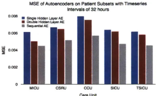
MSE of Autoencoders on Patert Subsets with Timeslere

Intm~at of 32 hours

0.005 U 00019081dde LayerAE

" Doul 1hidden LayerAEt

"* quibAE

0 gm

0.002

0.002

MICU CSRU CCU SICU TSICU

Care Unit

(b) Performance of autoencoders on patient

pop-ulation subsets with intervals of 32 hours.

Figure 5-2: Schematics of LSTM and CNN model architectures.

5.2

Results

5.2.1

Reconstruction Performance

We first evaluate the performance of each autoencoder by taking the mean squared error (MSE) between the predicted sequence of values and the true sequence of values. The sequential autoencoder with one LSTM layer achieves a lower MSE than the single-layer fixed length autoencoder on all interval lengths, but varies in comparison to the double-layer fixed length autoencoder (Figure 5-2a).

We also show that reconstructing input timeseries with autoencoders is fairly robust to stratifications in population subsets. We run the autoencoders on intervals of 32 hours with patient subsets stratified by care unit. MSEs are higher than when the autoencoders were trained on the entire patient population, but less than 0.08 in all cases, even though the training sets are much smaller (Figure 5-2b). On these smaller subsets of patients, the sequence autoencoder appears to be able to generalize to smaller amounts of training data and does better in all cases; in reconstructions, the sequence autoencoder appears less susceptible to signal noise.

1-layer autoencoder

LO bicarbonate

0.5 L

LIastollc blood pressure

cton inprd xgn

La

ascow coma scale total

0s MO J Meart rat* 1M atocft 1O potassium 0.0 sodium 0.s

I

%0 V

,,systolk blood pressure

LO tarmerature 10 1.0 0.51 0.0 2-layer autoencoder 1. bicarbonate 1.0 0.5 c.0 scl

um

Q.s 1.0 0.si 0.0 LO hematocrit 0.0 0 LO sodium 03s 0.01 A

Lytoi -blod pressure

O's "t F.-sequence autoencoder bicarbonate

I

SAM

j astolk blood pressure

00

taction inspired oxyg

1lascow coma scale total

43

0.0 LO heart rat

hematocrit

potassium

sodium

ystolIc blood pressure

10 Le enperature Ms LO wih M5 real predited

Figure 5-3: Examples of feature reconstructions for a single patient for an interval of

32 hours. Note that the scales for each variable are normalized between 0 and 1 based

on the population minimum and maximum. All autoencoders are able to predict the values of variables well, and the sequence autoencoder generally produces a smoother trajectory.

33 I

5.2.2

Predictive Ability

Accurately reconstructing the input demonstrates that a dense representation is able to capture important facets of the data. However, these facets should also have pre-dictive value. In the following chapter, we use the hidden representation from the sequence autoencoder to predict several clinical outcomes, and compare its perfor-mance along with a variety of other supervised representations.

Chapter 6

Actionable Intervention Prediction

We integrate data from all available ICU sources (vitals, labs, notes, demographics) and focus on learning rich representations of this data to predict onset and weaning of multiple invasive interventions. In particular, we compare autoencoder representa-tions, long short-term memory networks (LSTM) and convolutional neural networks

(CNN) for prediction of five intervention tasks: invasive ventilation, non-invasive

ventilation, vasopressors, colloid boluses, and crystalloid boluses.

Our predictions are done in a forward-facing manner to enable "real-time" per-formance, and predictions are made with a six hour gap time to support clinically actionable planning. We achieve state-of-the-art results on our predictive tasks using deep architectures.

6.1

Data Representation

Physiological variables, static data, and clinical text topics are extracted from MIMIC III as described in Chapter 4.

We compare forward-filled and normalized data ("raw" data) to physiological words, where we categorize the vitals data and topic distributions by first converting each value into a z-score based on the population mean and standard deviation for that

The work in this chapter was submitted to the 2017 Machine Learning for Healthcare Conference

with contributions from Nathan Hunt, Tristan Naumann, Alistair Johnson, Leo Celi, and Marzyeh Ghassemi.

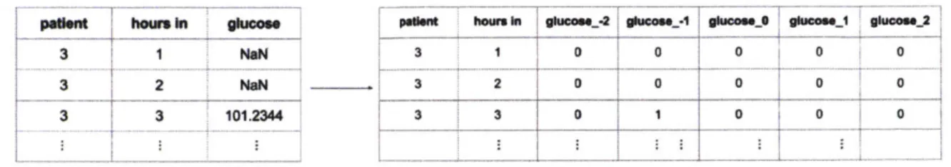
variable, and then rounding this score to the nearest integer and capping it to be between -4 and 4. Each z-score value then becomes its own column, which explicitly allows for a representation of missingness (e.g., all columns for a particular variable zeroed) that does not require imputation (Figure 6-1) [60].

Numerical Phys@logIcal Words

paet howrs in oiucone

3 1 N&M

3 2 Na

3 3 101.2344

Figure 6-1: Converting data from continuous timeseries format to discrete "physiolog-ical words." The numeric values are first z-scored and rounded, and then each z-score is made into its own category. On the right, glucose_-2 indicates the presence of a glucose value that was 2 standard deviations below the mean. A row containing all zeros for a given variable indicates that the value for that variable was missing at the timestep.

The physiological variables, topic distribution, and static variables for each pa-tient are concatenated into a single feature vector per papa-tient per hour [21]. The intervention state of each patient (a binary value indicating whether or not they are on the intervention of interest at each timestep) and the time of day for each timestep (an integer from 0 to 23 representing the hour) are also added to this feature vector. Using the time of day as a feature makes it easier for the model to capture circadian rhythms that may be present in, e.g., the vitals data.

6.2

Prediction Task

We split each patient's record into 6 hour chunks using a sliding window and make a prediction for a window of 4 hours after a gap time of 6 hours (Figure 6-2). When predicting ventilation, non-invasive ventilation, or vasopressors, the model classifies the prediction window as one of four possible outcomes: 1) Onset, 2) Wean, 3) Staying on intervention, 4) Staying off intervention. A prediction window is an onset if there is a transition from a label of 0 to 1 for the patient during that window; weaning is

36

peenut ho'' In Ouous-2 0UCae e" e..*1-j h'm". J ske'se*

3 1 0 0 0 0 0

3 2 0 0 0 0 0

PDetnt I)It

VQ

Signal (Y sklos size I'p nwIndow

FZZ1~

Figure 6-2: Given data from a fixed-length (6 hour) sliding window, models predict the status of intervention in a prediction window (4 hours) after a gap time (6 hours). Windows slide along the entire patient record, creating multiple examples from each record.

Onset Weaning Stay Off Stay On

Ventilation 0.005 0.017 0.798 0.180

Vasopressor 0.008 0.016 0.862 0.114

NI-Ventilation 0.024 0.035 0.695 0.246

Colloid Bolus 0.003 - -

-Crystalloid Bol 0.022 - -

-Table 6.1: The proportion of each intervention class. Note that colloid and crystalloid boluses are not administered for specific durations, and thus have only a single class

(onset). NI = non-invasive.

the opposite: a transition from 1 to 0. A window is classified as "stay on" if the label for the entire window is 1 or "stay off" if 0. When predicting colloid or crystalloid boluses, we classify the prediction window into one of two classes: 1) Onset, or 2) No Onset, since these interventions are not administered for on-going durations of time. After splitting the patient records into fixed-length chunks, we end up with 1,154,101 examples. Table 6.1 lists the proportions of each class for each intervention.

6.3

Methods

6.3.1

Long Short-Term Memory Network (LSTM)

We use long short-term memory networks (LSTM) as our first model, as described in Chapter 2. For a model schematic, see Figure 6-3a.

6.3.2

Convolution Neural Network (CNN)

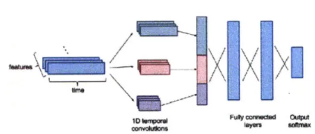
We employ a similar CNN architecture to [52], except that we do not initially convolve the features into an intermediate representation. We represent features as channels and perform 1D temporal convolutions, rather than treating the input as a 2D image. Our architecture consists of temporal convolutions at three different temporal granu-larities with 64 filters each. The dimensions of the filters are 1 x i, where i E {3, 4, 5}. We pad the inputs such that the outputs from the convolutional layers are the same size, and we use a stride of 1. Each convolution is followed by a max pooling layer with a pooling size of 3. The outputs from all three temporal granularities are concatenated and flattened

1571,

and followed by two fully connected layers with dropout in between and a softmax over the output (Figure 6-3b).

EZZ

(a) The LSTM consists of two hidden layers (b) The CNN architecture performs temporal

with 512 nodes each. We sequentially feed convolutions at 3 different granularities (3, 4,

in each hour's data. At the end of the ex- and 5 hours), max-pools and combines the out-ample window, we use the final hidden state puts, and runs this through 2 fully connected

to predict the output. layers to arrive at the prediction.

Figure 6-3: Schematics of LSTM and CNN model architectures.

6.3.3

Autoencoder Representations

We use the sequence autoencoder from Chapter 5 to generate representations in an

unsupervised framework, and compare these to the supervised representations that are learned in the neural network models. The autoencoder representation is of size

m

f

* k, where

f

is the number of features per timestep and k is the number of

timesteps being summarized. In a separate step, this representation is fed through a 2-layer feedforward neural network in order to predict the intervention class.

We compare representations trained to reconstruct either the numerical data (AE Raw) or the physiological words data (AE Words).

6.3.4

Experimental Settings

We use a train/validation/test split of 70/10/20 and stratify the splits based on .outcome. For the LSTM, we use dropout with a keep probability of 0.8 during

training (only on stacked layers), and L2 regularization with lambda = 1 x 10-4.

We use 2 hidden LSTM layers of 512 nodes each.. For the CNN, we use dropout between fully-connected layers with a keep probability of 0.5. For the feedforward neural net used to make predictions on the autoencoder representation, we use 2 layers of size 128 and 56. We use a weighted loss function during optimization to account for class imbalances. All parameters were determined using cross-validation with the validation set. We implemented all models in TensorFlow version 1.0.1 using the Adam optimizer on mini-batches of 128 examples. We determine when to stop training with early stopping based on the macro AUC on the validation set.

6.3.5

Evaluation

We evaluate our results based on per-class AUCs as well as aggregated macro AUCs.

If there are K classes each with a per-class AUC of AUCk then the macro AUC is

defined as the average of the per-class AUCS, AUC,, = ' Zk AUCk. We use the

macro AUC as an aggregate score because it weights the AUCs of all classes equally, regardless of class size

[44].

This is important because of the large class imbalance present in the data.

We use L2 regularized logistic regression (LR) as a baseline for comparison with the neural networks [51]. The same input is used as for the numerical LSTM and

CNN (imputed 6 hour chunks of data). 39

6.3.6

Interpretibility

LSTM Feature-Level Occlusions

Because of the additional time dependencies of recurrent neural networks, getting feature-level interpretability from LSTMs is notoriously difficult. To achieve this, we borrow an idea from image recognition to help understand how the LSTM uses different features of the patients. Zeiler et. al. use occlusion to understand how models process images: they remove a region of the image (by setting all values in that region to 0) and compare the model's prediction of this occluded image with the original prediction [64]. A large shift in the prediction implies that the occluded region contains important information for the correct prediction. With our LSTM model, we remove features one by one from the patients (by replacing the given feature with noise drawn from a uniform distribution in [0,1)). We then compare the predictive ability of the model with and without each feature; when this difference is large, then the model was relying heavily on that feature to make the prediction.

CNN Filter/Activation Visualization

We get interpretability from the CNN models in two ways. First, in order to un-derstand how the CNN is using the patient data to predict certain tasks, we find and compare the top 10 real examples that our model predicts are most and least likely to have a specific outcome. As our gap time is 6 hours, this means that the model predicts high probability of onset of the given task 6 hours after the end of the identified trajectories.

Second, we generate "hallucinations" from the model which maximize the predicted probability for a given task [20]. This is done by creating an objective function that maximizes the activation of a specific output node, and backpropagating gradients back to the input image, adjusting the image so that it maximally activates the output node.

6.4

Results

We found deep architectures achieved state-of-the-art prediction results for our inter-vention tasks. The AUCs for each of our five interinter-vention types and 4 prediction tasks are shown for all models in Table 6.2. All models use 6 hour chucks of "raw" data which have either been transformed to a 0-1 range (normalized and mean imputed), or discretized into physiological words (Section 6.1).

6.4.1

Physiological Words Improve Predictive Task

Perfor-mance With High Class Imbalance

We observed a significantly increased AUC for some interventions when we used physiological words - specifically for ventilation onset (from 0.61 to 0.75) and colloid bolus onset (from 0.52 to 0.72), which have the lowest proportion of onset examples (Table 6.1). This may be because physiological words have a smoothing effect. Since we round the z-score for each value to the nearest integer, if a patient has a heart rate of 87 at one hour and then 89 at the next, those will probably be represented as the same word. This may make the model invariant to small fluctuations in the patient's data and more resilient to overfitting small classes. In addition, the physiological word representation has an explicit encoding for missing data. This is in contrast to the raw data that has been forward-filled and mean-imputed, introducing noise and making it difficult for the model to know how confident to be in the measurements it is given [8]. It may be for the same reason that the autoencoder representation trained on physiological words also equal to or better on all tasks than the autoencoder for numerical values.

6.4.2

Feature-Level Occlusions Identify Important Per-Class

Features

We are able to interpret the LSTM's predictions using feature occlusion (Section 4.5.1). We note that vitals, labs, topics and static data are important for different

interventions (Figure 6-4). Table A. 1 has words for each topic mentioned.

Ventilation Onset Ventilation Weaning

a complete listing of the most probable

Vasopressor Onset Vasopressor Weaning

0.12 -030 - E010 0.0175 .10.014 00.0.2s . 0.2 - 0.1 0.0125-.0 - *2 . 0.1 - Mo00075 000

Ii.i1

-

I

0.00 0,04 - 0.0 ~ E4- 0.07-002 _U m .04 - 0.0025 -(N ) f) (g) (d)

t 0sks- Vntionnse NIVentilaton W-enn 6-4f) sdalid bolusnes (6-4, lo4h) ote that

00O2 QO051 0 100 0,02

all wenn tak ecp frvntltonhv0sgiicnl -es-ACvran.

in

In

ne (H oim lactate, eoliian

0oasu)

Ilhisssesb,

0.000 1 00000

E~ . 00Ef

V

I

bAUs for eah interetintask Ine generassstn' physiological daawrsmrmtat for thentmo inagesive intervention.mehnialverntiltiion 6-aset4b advso-a praesr (mp-tce -4d whpaiet' clcasgoe toic were (GCr ) ipant for le(ssesvsive

0tas ntion- inasive veNtlation 4e 6-f aC frid Bolusnet w4 t4h) Notnset all weaning ts texcet for veilaio have sirifiany ae d AUC varane.

For0 mehnia vetiaton, th to five imotn fetue 2aecosstn1frwen

in asr onset reddumlctate, physmoglobina, arbdssha potassiumi sensile

peattr conssesstikly bpcrasntwint seationes at critical artsofsmecthafcal

adwaninga ste larg stmobrved (pi t or an nd0.12 falne).

In ~ ~ 4000 vaorso ne rdcin hsooia vrale uhasptssu n

hemaocri are41 cosstnl imorat, whc agrees wit clnclasesetfcr

divacua stt [2] Siiary Toi 3 (noin man phsooia vle)Isnls

important for both onset and weaning. Note that the overall difference in AUC for onset ranges up to 0.16, but there is no significant decrease in AUC for weaning (< 0.02). This is consistent with previous work that demonstrated weaning to be a more difficult task in general for vasopressors 160]. We also note that weaning prediction places importance on time of day. As noted by [60], this could be a side-effect of patients being left on interventions longer than necessary.

For non-invasive ventilation onset and weaning the learned topics are more im-portant than physiological variables. This may mean that the need for less severe interventions can only be detected from clinical insights derived in notes. Similarly to vasopressors, we note that onset AUCs vary more than weaning AUCs (0.14 vs

0.01), and that time of day is important for weaning.

For crystalloid and colloid bolus onsets, topics are all but one of the five most important features for detection. Colloid boluses in general have more AUC variance for the topic features (0.14 vs. 0.05), which is likely due to the larger class imbalance compared to crystalloids.

6.4.3

Convolutional Filters Target Short-term Trajectories

We are able to understand the CNN by examining maximally activating patient tra-jectories (Section 4.5.2). Figure 6-5 shows the mean with standard deviation error bars four features of the 10 real patient trajectories that are the highest and lowest activating for each task. The trends suggest that patients who will require ventilation in the future have higher diastolic blood pressure, respiratory rate, and heart rate, and lower oxygen saturation - possibly corresponding to patients who are experiencing hyperventilation. For vasopressor onsets, we see a decreased systolic blood pressure, heart rate and oxygen saturation rate. These could either indicate altered peripheral perfusion or stress hyperglycemia. Topic 3, which was important for vasopressor onset using occlusion 6-4, is also increased.

In the less invasive tasks, we saw decreased creatinine, phosphate, oxygen sat-uration and blood urea nitrogen for non-invasive ventilation, potentially indicating neuromuscular respiratory failure. For colloid and crystalloid boluses we note general

VgnWUMa Mmope" Non-. MVnt

diastolic BP heart rate blood urea nitrogen

100 12

60 75 30

40

6

0

heart rate i satationt

1 230 43

0 so L

12

- top 10 tragectorIes

- bottor 10 trajectorIes

Figure 6-5: Trajectories of the 10 maximally and

onset of each of the interventions.

CoNOW BOAMu

blood 4re nItrgen

0 oxyge sobatimt n =4 200 75 C lyiptor rates 2S 0 Soxygen saturation D2 -0

minimally activating examples for

indicators of physiological decline, as boluses are given for a wide range of conditions. While we observe many differences in value, the trajectories do not display sig-nificant trends (i.e. spikes, increases, decreases), suggesting that an absolute value being higher or lower is more important than the way that value fluctuates in the short term.

"Hallucinations" for vasopressor and ventilation onset are shown in Figure 6-6. While our model was not trained with any physiological knowledge or priors, we note that it identifies blood pressure drops as being maximally activating for vasopressor onset, and respiratory rate decreasing for ventilation onset. This suggests that it is still able to independently learn physiological factors that are important for in-tervention prediction. We note that these hallucinations give us more insight into underlying properties of the network and what it is looking for. However, since these trajectories are made to maximize the output of the model, they do not necessarily correspond to physiologically plausible trajectories.

heat ratu -twn ep

-vawopresw or*Mse

-- ventlanon onvm*

Figure 6-6: Trajectories generated by adjusting inputs to maximally activate a specific output node of the CNN.

Task Model

Intervention Type

VENT NI-VENT VASO COL BOL CRYS BOL

Baseline 0.60 0.66 0.43 0.65 0.67

o

l i LSTM Raw 0.61 0.75 0.77 0.52 0.70 LSTM Words 0.75 0.76 0.76 0.72 0.71 CNN 0.62 0.73 0.77 0.70 0.69 AE Raw 0.56 0.71 0.73 0.61 0.62 AE Words 0.61 0.72 0.73 0.66 0.64 d 0 Baseline 0.83 0.71 0.74 - -LSTM Raw 0.90 0.80 0.91 - -LSTM Words 0.90 0.81 0.91 - -CNN 0.91 0.80 0.91 - -AE Raw 0.88 0.78 0.90 - -AE Words 0.90 0.79 0.90 -Baseline 0.50 0.79 0.55 - -2 0

<

LSTM Raw 0.96 0.86 0.96 -LSTM Words 0.97 0.86 0.95 - -CNN 0.96 0.86 0.96 -AE Raw 0.95 0.85 0.94 -AE Words 0.96 0.85 0.94 -Baseline 0.94 0.71 0.93 - -c 0

<

LSTM Raw 0.95 0.86 0.96 - -LSTM Words 0.97 0.86 0.95 - -CNN 0.95 0.86 0.96 - -AE Raw 0.95 0.80 0.92 - -AE Words 0.95 0.83 0.92 -Baseline LSTM Raw LSTM Words CNN AE Raw AE Words 0.72 0.86 0.90 0.86 0.84 0.85 0.72 0.82 0.82 0.81 0.78 0.80 0.66 0.90 0.89 0.90 0.87 0.87

Table 6.2: Comparison of model performance on five targeted interventions. Models that perform best for a given (intervention, task) pair are bolded.

45

SYStwnc SP

6.4.4

Supervised Representations Outperform Unsupervised

Previous work has shown that intermediate layers of neural networks are able to learn a robust hierarchy of representations of the input [49].

We find that the representations learned within our supervised CNN and LSTM networks perform better than the unsupervised representations learned by the au-toencoders. While supervised learning tasks risk learning features too specific to a single task, we posit that our networks are not as susceptible to overfitting due to the fact that we predict not just onset, but all parts of the patient trajectory. Using regularization, dropout, and many hidden units likely improves these representations as well.