Chemical Abundances of New Member Stars in the Tucana II Dwarf Galaxy

(1)

Chemical Abundances of New Member

Stars in the Tucana II Dwarf Galaxy

The MIT Faculty has made this article openly available. Please share

how this access benefits you. Your story matters.

Citation

Chiti, Anirudh et al “Chemical Abundances of New Member Stars in

the Tucana II Dwarf Galaxy.” The Astrophysical Journal 857, 1 (April

2018): 74 © 2018 American Astronomical Society

As Published

http://dx.doi.org/10.3847/1538-4357/AAB4FC

Publisher

American Astronomical Society

Version

Final published version

Citable link

http://hdl.handle.net/1721.1/117552

Terms of Use

Article is made available in accordance with the publisher's

policy and may be subject to US copyright law. Please refer to the

publisher's site for terms of use.

(2)

Chemical Abundances of New Member Stars in the Tucana II Dwarf Galaxy

∗

Anirudh Chiti1 , Anna Frebel1 , Alexander P. Ji2,5, Helmut Jerjen3 , Dongwon Kim4, and John E. Norris3

1

Department of Physics and Kavli Institute for Astrophysics and Space Research, Massachusetts Institute of Technology, Cambridge, MA 02139, USA

achiti@mit.edu

2

Observatories of the Carnegie Institution of Washington, 813 Santa Barbara Street, Pasadena, CA 91101, USA

3

Research School of Astronomy and Astrophysics, Australian National University, Canberra, ACT 2611, Australia

4

Astronomy Department, University of California, Berkeley, CA, USA

Received 2017 December 23; revised 2018 February 20; accepted 2018 March 2; published 2018 April 16

Abstract

We present chemical abundance measurements for seven stars with metallicities ranging from Fe/H]=−3.3 to

[Fe/H]=−2.4 in the Tucana II ultra-faint dwarf galaxy (UFD), based on high-resolution spectra obtained with the MIKE spectrograph on the 6.5 m Magellan-Clay Telescope. For three stars, we present detailed chemical

abundances for theﬁrst time. Of those, two stars are newly discovered members of Tucana II and were selected as

probable members from deep narrowband photometry of the Tucana II UFD taken with the SkyMapper telescope. This result demonstrates the potential for photometrically identifying members of dwarf galaxy systems based on chemical composition. One new star was selected from the membership catalog of Walker et al. The other four stars in our sample have been reanalyzed, following additional observations. Overall, six stars have chemical abundances that are characteristic of the UFD stellar population. The seventh star shows chemical abundances that are discrepant from the other Tucana II members and an atypical, higher strontium abundance than what is expected for typical UFD stars. While unlikely, its strontium abundance raises the possibility that it may be a foreground metal-poor halo star with the same systemic velocity as Tucana II. If we were to exclude this star,

Tucana II would satisfy the criteria to be a survivingﬁrst galaxy. Otherwise, this star implies that Tucana II has

likely experienced somewhat extended chemical evolution.

Key words: galaxies: dwarf– galaxies: individual (TucII) – Local Group – stars: abundances

Supporting material: machine-readable tables

1. Introduction

The elements in the atmospheres of metal-poor stars allow us to study the chemical composition of the early universe. The

elements in stellar atmospheres reﬂect the composition of a

star’s formative gas cloud. Thus, a low surface metal

abundance of a metal-poor star indicates its natal gas cloud must have undergone relatively few cycles of chemical

enrichments (e.g., from supernovae). This lack of enrichment

implies that metal-poor stars generally formed earlier than typical solar-metallicity stars, and that metal-poor stars can be used to probe the composition of the early universe in which they formed.

The iron abundance is typically used as a proxy for the overall

metal context(or “metallicity”) of a star and metal-poor stars are

deﬁned to have an iron abundance of[Fe H] -1 dex, where

[Fe/H]=log10(NFe NH) -log10(NFe NH) (Frebel & Norris

2015). Of particular interest are the most metal-poor stars, such as

very metal-poor stars (VMP;[Fe H]  -2.0) and extremely

metal-poor stars (EMP; [Fe H]  -3.0). The abundance of

various elements (i.e., carbon, neutron-capture elements) as a

function of overall[Fe/H] for VMP and EMP stars sheds light on

the nature of the chemical evolution of the early universe(Sneden

et al.1996; Beers & Christlieb2005; Placco et al.2014; Roederer

et al.2014). Stars with[Fe H] -4.0 can be used to constrain

the yields and properties of the veryﬁrst supernovae (e.g., Heger

& Woosley 2010) and, by extension, the properties of the ﬁrst

stars(Bromm et al.2009). Metal-poor stars have also been used to

trace old substructure in the Milky Way (e.g., Starkenburg

et al. 2017), and to address a number of questions related to

galaxy formation and cosmology(Spite & Spite1982; Freeman &

Bland-Hawthorn2002; Frebel et al.2007; Frebel & Norris2013,

2015; Karlsson et al.2013).

The simpler formation history of dwarf galaxies makes them an ideal laboratory to use metal-poor stars for studying topics such as chemical evolution, star formation history, and stellar

populations (Tolstoy et al. 2009). Furthermore, faint dwarf

galaxies are thought to be the surviving analogs of the ancient

galaxies that were accreted to form the Milky Way halo(Frebel

et al. 2010a; Belokurov 2013), and are also themselves older

and more metal-poor than some components of the Milky Way,

such as the disk(Simon & Geha2007; Kirby et al.2013). Thus,

studying the metal-poor stars in these systems provides insights

on the nature of the ﬁrst galaxies and the origins of the of

chemical signatures of the VMP and EMP stellar population in

the halo(Starkenburg & Helmi2015).

Ultra-faint dwarf galaxies(UFDs), in particular, are among the

oldest(10 Gyr), most metal-poor (typically a mean[Fe H]<

-2.0), and dark-matter dominated (M/LV100) (e.g., Brown

et al.2014) dwarf galaxy systems. These characteristics make stars

in UFDs especially promising targets for studying the aforem-entioned questions. Several surveys over the past decade have

detected dozens of UFDs(Willman et al.2005; Zucker et al.2006;

Belokurov et al.2007; Walsh et al.2007; Willman2010; Bechtol

et al.2015; Drlica-Wagner et al.2015,2016; Kim & Jerjen2015;

Kim et al. 2015; Koposov et al. 2015; Laevens et al. 2015a,

2015b; Homma et al. 2016, 2018), thus greatly increasing the

prospect for studying the population of metal-poor stars in their environments.

∗_{This paper includes data gathered with the 6.5 m Magellan Telescopes}

located at Las Campanas Observatory, Chile.

5

(3)

To investigate the detailed chemical composition of stars, it is necessary to obtain high-resolution spectra. Results already show the utility of detailed studies of the composi-tion of metal-poor stars in UFDs. For instance, the strong overabundance of neutron-capture elements associated with the r-process in seven stars in the Reticulum II UFD has constrained the dominant astrophysical site of the r-process

(Ji et al.2016a). However, only 59 stars have been observed

with high-resolution spectroscopy in 14 UFD systems

(Koch et al. 2008,2013; Feltzing et al. 2009; Frebel et al.

2010a, 2010b, 2014; Norris et al. 2010a, 2010b; Simon

et al.2010; Gilmore et al.2013; Ishigaki et al.2014; Koch &

Rich 2014; Roederer & Kirby2014; Ji et al.2016b,2016c,

2016d; Hansen et al. 2017; Kirby et al. 2017; Venn et al.

2017; Nagasawa et al. 2018) because the low stellar mass

(104M), distance (d30 kpc), and lack of giant branch

stars in UFDs (e.g., Martin et al. 2008) strictly limits the

stars for which high-resolution spectroscopy can be per-formed with current technology. Adding to the observational burden, medium-resolution spectroscopy is required to

identify which stars in their ﬁeld are members of these

systems before high-resolution observations can be carried out. All of these reasons make the time required to identify and observe member stars of UFDs a bottleneck to progress

in theﬁeld.

In this paper, we present the chemical abundances of seven

stars with[Fe/H] ranging from −2.4 to −3.3 dex in the UFD

Tucana II(Bechtol et al. 2015; Koposov et al.2015) derived

from high-resolution spectroscopy. Two stars are new

members that were identiﬁed from photometry of the Tucana

II dwarf galaxy obtained with theﬁlter set on the SkyMapper

telescope(A. Chiti et al. 2018, in preparation). The discovery

of these stars motivated studying Tucana II in more detail. We

also observed one new star that was previously conﬁrmed

as a member by Walker et al. (2016). To supplement the

new observations, we decided to re-analyze the four stars

with published measurements from Ji et al. (2016b), after

collecting additional data to improve measurement precision. As observations suggest that UFDs contain no members with [Fe/H]>−1, selecting metal-poor stars from photometry is a

potentially powerful way to identify signiﬁcant numbers of

UFD members for spectroscopic follow-up observations. This has the potential for bypassing the expensive medium-resolution spectroscopy step of the process, thus accelerating the characterization of UFDs and other dwarf galaxies.

This paper is organized as follows. We outline the target

selection procedure and observations in Section 2; discuss the

abundance analysis in Section 3; present the chemical

signatures of stars in Tucana II and implications in

Sections4; and conclude in Section5.

2. Target Selection and Observations

2.1. Members from Walker et al.(2016)

Ji et al.(2016b) observed TucII-006, TucII-011, TucII-033,

and TucII-052 with the MIKE spectrograph(see Table1). All

four stars were selected from the membership catalog of

Walker et al. (2016). They observed each star between

100 minutes to 4.42 hr in 2016 August with the MIKE spectrograph on the Magellan-Clay telescope. For the stars

with the shortest exposure times (TucII-033 and TucII-052),

this precluded the measurement of several elements and led to

large uncertainties in the measurement of the abundances of several other elements. Thus, we re-observed each star in Ji

et al. (2016b) for an additional 55 minutes to address the

aforementioned deﬁciencies. In addition to re-observing these

stars, we observed an additional member (TucII-078) from

Walker et al.(2016) that had not previously been observed with

a high-resolution spectrograph.

2.2. Members Selected from SkyMapper Photometry Through a P.I. program, we obtained SkyMapper photometry of Tucana II using the 1.3 m telescope at Siding Spring Observatory. In an upcoming paper, we will fully discuss the

implementation of the SkyMapper ﬁlter set to determine

photometric metallicities (A. Chiti et al. 2018, in preparation),

but we brieﬂy discuss the method here. The SkyMapper ﬁlter set

includes a narrowband vﬁlter that covers the prominent CaIIK

line at 3933.7Å (Bessell et al.2011). Given the strength of this

line, the preponderance or lack of metals sufﬁciently affects the

line strength which changes the totalﬂux through this ﬁlter. Thus,

a metal-poor star with a weak CaIIK line appears brighter in this

ﬁlter than more metal-rich stars. To quantify this effect, we

generated a grid of ﬂux-calibrated spectra using the

Turbospec-trum synthesis code (Alvarez & Plez 1998; Plez 2012), the

MARCS model atmospheres(Gustafsson et al.2008), and a line

list derived from the Vienna Atomic Line Database (VALD)

(Piskunov et al. 1995; Ryabchikova et al. 2015). The stellar

parameters of our grid covered the expected stellar parameters (4000<Teff[ ]K <5700; 1<logg<3) and metallicities

(-4.0<[Fe H]< -0.5) of RGB stars in dwarf galaxies. We

closely followed the methodology of Bessell & Murphy(2012)

and Casagrande & VandenBerg(2014) to generate a library of

synthetic photometry through the SkyMapper u, v, g, and iﬁlters

for spectra in this grid.

By relating our observed SkyMapper photometry in the v, g,

and i ﬁlters to the synthetic photometry from our grid, we

selected a few metal-poor targets for spectroscopic test

observations. Two of these targets (TucII-203 and TucII-206)

were conﬁrmed as members of Tucana II since radial velocity

measurements from their Magellan Inamori Kyocera Echelle (MIKE) spectra were similar to the systemic velocity of Tucana

II of−129.1 km s−1(Walker et al.2016).

2.3. High-resolution Spectroscopy

The data in this paper were obtained with the MIKE spectrograph on the Clay telescope at Las Campanas

Observatory (Bernstein et al. 2003). The observations were

taken between 2017 August 14–17 and October 7–11.

Examples of the spectra are shown in Figure 1. The location

of each star in the color–magnitude diagram of Tucana II is

shown in Figure2. Targets were observed with 2×2 binning

and the 1 0 slit(R∼28,000 on the blue chip and R∼22,000

on the red chip) covering ∼3500 Å to ∼9000 Å. The weather

was mostly clear on all nights. The spectra were all reduced and

wavelength calibrated with the MIKE CarPy pipeline6

(Kelson2003).

6

(4)

Table 1 Observations

Name R.A.(h:m:s) (J2000) Decl.(d:m:s) (J2000) Slit Size g(mag) texp(minutes) S/N

a vhelio(km s−1) TucII-006 22:51:43.06 −58:32:33.7 1 0 18.78 206b 15, 30 −126.1 TucII-011 22:51:50.28 −58:37:40.2 1 0 18.27 314b 15, 30 −124.6 TucII-033 22:51:08.32 −58:33:08.1 1 0 18.68 155b 17, 32 −126.9 TucII-052 22:50:51.63 −58:34:32.5 1 0 18.83 155b 17, 35 −119.9 TucII-078 22:53:06.67 −58:31:16.0 1 0 18.62 215 15, 30 −123.8 TucII-203 22:50:08.87 −58:29:59.1 1 0 18.81 275 16, 37 −126.1 TucII-206 22:54:36.67 −58:36:57.9 1 0 18.81 385 15, 37 −122.9 Notes. a

Signal-to-noise(S/N) per pixel is listed for 4500 and 6500 Å.

b_{Combined exposure time from Ji et al.}₍_2016b_{) and this work.}

Figure 1.Plots of the CH region(left), Mg b line region (center), and Hα feature (right) for each of the Tucana II members with no prior high-resolution chemical abundance measurements available. TucII-078 was spectroscopically identiﬁed as member (Walker et al.2016), while TucII-203 and TucII-206 were identiﬁed based

on narrowband photometry.

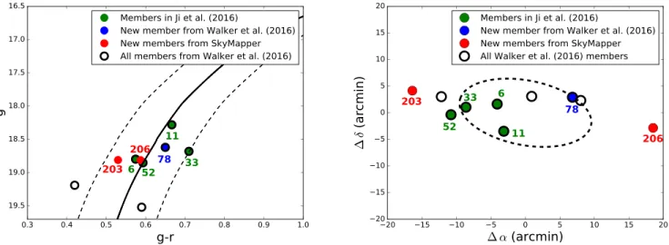
Figure 2.Left: color-magnitude diagram of TucII stars from this study. A Dartmouth isochrone(Dotter et al.2008) with an age of 12.5 Gyr, distance modulus of

18.8, and a metallicity of[Fe H/ ]= -2.5 is overplotted in black along with offsets of(g−r)±0.1 in dashed lines to guide the eye. We denote with different colors the four members previously observed by Ji et al.(2016b), one member selected from Walker et al. (2016), and two selected from our SkyMapper

photometry. Open circles indicate conﬁrmed members in Walker et al. (2016) with no high-resolution spectroscopic observations. Right: spatial distribution of

TucII members centered on the coordinates of Tucana II. The elliptical half-light radius from Koposov et al.(2015) is overplotted. In both plots, each star is

(5)

3. Abundance Analysis 3.1. Derivation of Stellar Parameters

and Chemical Abundances

The Python-based Spectroscopy Made Hard analysis

soft-wareﬁrst described in Casey (2014) was used for the majority

of our analysis, including normalizing spectra, measuring equivalent widths, and generating synthetic spectra. Our version of this software made use of the 2011 version of

MOOG (Sneden 1973), which has an updated treatment of

scattering from Sobeck et al. (2011). The spectroscopic stellar

parameter adjustment scheme by Frebel et al. (2013) is based

on this version. We usedα-enhanced, 1D plane-parallel stellar

model atmospheres from Castelli & Kurucz (2004). The line

list in Roederer et al.(2014) was used for identifying lines and

deriving abundances from equivalent width measurements. For spectral syntheses, we supplemented this line list with those

used in Ji et al. (2016d). Namely, we incorporated lines from

Hill et al.(2002), Den Hartog et al. (2003), Ivans et al. (2006),

Lawler et al.(2006,2009), Sneden et al. (2009), and Masseron

et al.(2014). Our chemical abundances are listed relative to the

solar abundances of Asplund et al. (2009).

We derived radial velocities by cross correlating our observed spectra with a template spectrum of HD 140283 over

the Hβ feature at 4861 Å. Heliocentric velocity corrections

were derived using the rvcorrect task in the Image Reduction and Analysis Facility (IRAF)

soft-ware. We ﬁnd evidence that TucII-078 may be in a binary,

since our measured velocity is ∼12 km s−1 greater than the

velocity reported in Walker et al.(2016).

We determined stellar parameters and chemical abundances

following Frebel et al. (2013) whose methodology we brieﬂy

outline in this paragraph. First, equivalent widths were

measured by ﬁtting a Gaussian proﬁle to each line. We

generally excluded lines with reduced equivalent width

measurements greater than −4.5, as these measurements

potentially lie outside the linear regime of the curve of growth.

We varied the stellar parameters(Teff, log g, vmicro, and[Fe/H])

until our FeIabundances showed no trend with both excitation

potential and reduced equivalent width. We further constrained

log g by requiring our FeIand FeIIabundances to match. We

then corrected our Teff with the prescription given in Frebel

et al.(2013), but readjusted log g, vmicro, and[Fe/H] until the

above criteria were again satisﬁed. To determine random

uncertainties, stellar parameters were varied to match the 1σ

uncertainty in the FeI abundance trends. These random

uncertainties were added in quadrature to the systematic

uncertainties, which were assumed to be 150 K for Teff,

0.3 dex for log g, and 0.2 km s−1 for vmicro. The ﬁnal stellar

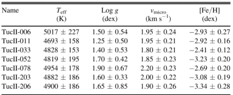
parameter measurements are listed in Table 2.

We followed a few prescriptions to determine uncertainties for abundances based on equivalent width measurements. For

abundances measured with a large number of lines(N10),

we take the standard deviation of the individual line abundances as the random uncertainty. We adopt the standard deviation as it well represents abundance uncertainties obtained

from data with poor signal-to-noise (S/N). For abundances

with a small number of lines (1<N<10), we derived

random uncertainties by multiplying the range covered by the

line abundances by the k-statistic following Kenney(1962) to

obtain a standard deviation. The k-statistic gives measurements with a smaller number of lines an appropriately larger uncertainty. For abundances derived from only one line measurement, we derived the random uncertainty by varying the continuum placement and assuming the resulting abun-dance variation as the uncertainty. If any resulting random uncertainty was below the standard deviation of the abundances of the iron lines, we nominally adopt as a conservative random uncertainty the standard deviation of the iron abundance (0.12–0.27 dex). The total uncertainty for each element was then determined by adding the random uncertainty in quadrature with the systematic uncertainties. The systematic uncertainties were assumed to be the difference in the abundances caused by varying each stellar parameter by its

1σ uncertainty.

For abundances measured by spectrum syntheses, we also derived uncertainties by adopting the procedure in the previous paragraph. If an element had only one synthesized line, the random uncertainty was assumed to be the change in abundance that was required to capture the variations of the continuum placement. The systematic uncertainty was obtained by measuring the change in the abundance after varying each

stellar parameter by its 1σ uncertainty. If an element had

measured abundances from both spectrum synthesis and equivalent width measurements, we pooled the measurements and derived random uncertainties following the procedure outlined in the previous paragraph. The random uncertainty was then added in quadrature with the systematic uncertainties for each star to derive a total uncertainty. Certain elements (e.g., Al and Si) had absorption features that were detected in

our data, but the S/N was too poor to derive a meaningful

abundance and especially uncertainty. However, we report

tentative abundances but mark them with a colon in Table3to

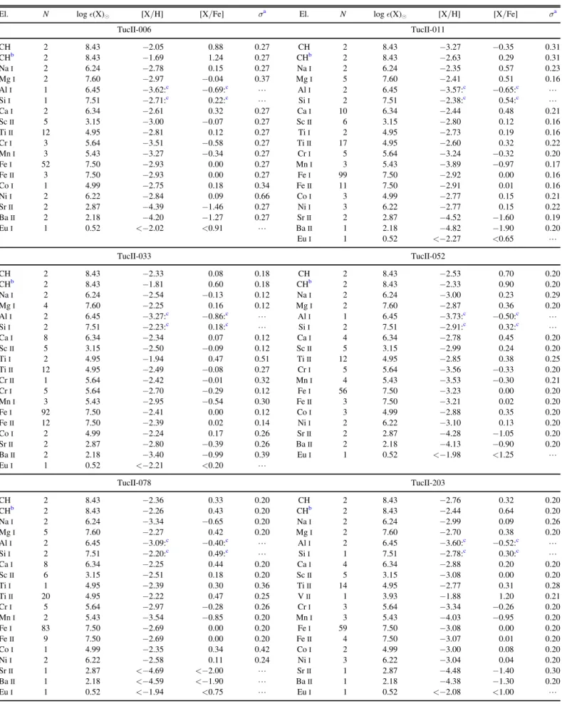
indicate a large uncertainty. Our measurements and

uncertain-ties are listed in Tables 3 and 4. Our individual equivalent

width and synthesis measurements are listed in Table5.

3.2. Comparison with Ji et al.(2016b) and Walker et al. (2016)

We compare our results with measurements from Ji et al. (2016b) and Walker et al. (2016) to check consistency with

previous studies of Tucana II. We focus on comparisons with Ji

et al. (2016b), with whom we have four stars in common, as

they also analyzed high-resolution spectra from the MIKE spectrograph.

Weﬁrst discuss our measured stellar parameters and chemical

abundances of TucII-006, TucII-011, TucII-033, and TucII-052 in

comparison with those presented in Ji et al.(2016b). For TucII-011

and TucII-052, weﬁnd excellent agreement (within 1σ) in stellar

parameters and chemical abundances. For TucII-006, we measure

a discrepant log g by 0.4±0.4 dex, a discrepant microturbulence

by 0.25±0.26 dex, and a discrepant [Fe/H] by 0.25±0.21 dex,

where the uncertainties are from Ji et al. (2016b). However,

Table 2 Stellar Parameters

Name Teff Log g vmicro [Fe/H]

(K) (dex) (km s−1₎ _(dex) TucII-006 5017±227 1.50±0.54 1.95±0.24 −2.93±0.27 TucII-011 4693±158 1.25±0.50 1.95±0.21 −2.92±0.16 TucII-033 4828±153 1.40±0.53 1.80±0.21 −2.41±0.12 TucII-052 4819±195 1.70±0.42 1.85±0.23 −3.23±0.20 TucII-078 4954±178 1.90±0.67 2.20±0.23 −2.69±0.20 TucII-203 4882±186 1.60±0.33 2.00±0.22 −3.08±0.19 TucII-206 4900±186 1.65±0.85 1.90±0.26 −3.34±0.28

(6)

Table 3 Chemical Abundances

El. N logò(X)e [X/H] [X/Fe] σa El. N logò(X)e [X/H] [X/Fe] σa

TucII-006 TucII-011 CH 2 8.43 −2.05 0.88 0.27 CH 2 8.43 −3.27 −0.35 0.31 CHb 2 8.43 −1.69 1.24 0.27 CHb 2 8.43 −2.63 0.29 0.31 NaI 2 6.24 −2.78 0.15 0.27 NaI 2 6.24 −2.35 0.57 0.23 MgI 2 7.60 −2.97 −0.04 0.37 MgI 5 7.60 −2.41 0.51 0.16 AlI 1 6.45 −3.62:c −0.69:c L AlI 2 6.45 −3.57:c −0.65:c L SiI 1 7.51 −2.71:c 0.22:c L SiI 2 7.51 −2.38:c 0.54:c L CaI 2 6.34 −2.61 0.32 0.27 CaI 10 6.34 −2.44 0.48 0.21 ScII 5 3.15 −3.00 −0.07 0.27 ScII 6 3.15 −2.80 0.12 0.16 TiII 12 4.95 −2.81 0.12 0.27 TiI 2 4.95 −2.73 0.19 0.16 CrI 3 5.64 −3.51 −0.58 0.27 TiII 17 4.95 −2.60 0.32 0.22 MnI 3 5.43 −3.27 −0.34 0.27 CrI 5 5.64 −3.24 −0.32 0.20 FeI 52 7.50 −2.93 0.00 0.27 MnI 3 5.43 −3.89 −0.97 0.17 FeII 3 7.50 −2.93 0.00 0.27 FeI 99 7.50 −2.92 0.00 0.16 CoI 1 4.99 −2.75 0.18 0.34 FeII 11 7.50 −2.91 0.01 0.16 NiI 2 6.22 −2.84 0.09 0.66 CoI 3 4.99 −2.77 0.15 0.21 SrII 2 2.87 −4.39 −1.46 0.27 NiI 3 6.22 −2.77 0.15 0.22 BaII 2 2.18 −4.20 −1.27 0.27 SrII 2 2.87 −4.52 −1.60 0.19 EuI 1 0.52 <−2.02 <0.91 L BaII 1 2.18 −4.82 −1.90 0.20 EuI 1 0.52 <−2.27 <0.65 L TucII-033 TucII-052 CH 2 8.43 −2.33 0.08 0.18 CH 2 8.43 −2.53 0.70 0.20 CHb 2 8.43 −1.81 0.60 0.18 CHb 2 8.43 −2.33 0.90 0.20 NaI 2 6.24 −2.54 −0.13 0.12 NaI 2 6.24 −3.00 0.23 0.29 MgI 4 7.60 −2.25 0.16 0.12 MgI 2 7.60 −2.87 0.36 0.20 AlI 2 6.45 −3.27:c −0.86:c L AlI 1 6.45 −3.73:c −0.50:c L SiI 2 7.51 −2.23:c 0.18:c L SiI 2 7.51 −2.91:c 0.32:c L CaI 8 6.34 −2.34 0.07 0.12 CaI 4 6.34 −2.78 0.45 0.20 ScII 5 3.15 −2.50 −0.09 0.12 ScII 5 3.15 −2.99 0.24 0.20 TiI 2 4.95 −1.94 0.47 0.51 TiII 12 4.95 −2.85 0.38 0.25 TiII 12 4.95 −2.49 −0.08 0.27 CrI 5 5.64 −3.56 −0.33 0.20 CrII 1 5.64 −2.42 −0.01 0.32 MnI 4 5.43 −3.53 −0.30 0.21 CrI 5 5.64 −2.70 −0.29 0.12 FeI 56 7.50 −3.23 0.00 0.20 MnI 3 5.43 −2.95 −0.54 0.30 FeII 3 7.50 −3.21 0.02 0.20 FeI 92 7.50 −2.41 0.00 0.12 CoI 3 4.99 −2.88 0.35 0.20 FeII 12 7.50 −2.39 0.02 0.14 NiI 2 6.22 −3.10 0.13 0.20 CoI 2 4.99 −2.24 0.17 0.26 SrII 2 2.87 −4.28 −1.05 0.20 SrII 2 2.87 −2.80 −0.39 0.26 BaII 2 2.18 −4.13 −0.90 0.20 BaII 2 2.18 −3.40 −0.99 0.39 EuI 1 0.52 <−1.98 <1.25 L EuI 1 0.52 <−2.21 <0.20 L TucII-078 TucII-203 CH 2 8.43 −2.36 0.33 0.20 CH 2 8.43 −2.76 0.32 0.20 CHb 2 8.43 −2.26 0.43 0.20 CHb 2 8.43 −2.44 0.64 0.20 NaI 2 6.24 −3.34 −0.65 0.20 NaI 2 6.24 −2.99 0.09 0.26 MgI 5 7.60 −2.27 0.42 0.20 MgI 2 7.60 −2.70 0.38 0.20 AlI 2 6.45 −3.09:c _−0.40:c _L _Al_I ₂ _6.45 _−3.60:c _−0.52:c _L SiI 2 7.51 −2.20:c 0.49:c L SiI 1 7.51 −2.78:c 0.30:c L CaI 8 6.34 −2.25 0.44 0.20 CaI 4 6.34 −2.88 0.20 0.20 ScII 6 3.15 −2.51 0.18 0.20 ScII 5 3.15 −3.08 0.00 0.20 TiI 1 4.95 −2.39 0.30 0.36 TiII 14 4.95 −2.77 0.31 0.28 TiII 20 4.95 −2.22 0.47 0.25 VII 1 3.93 −1.88 1.20 0.21 CrI 5 5.64 −2.97 −0.28 0.26 CrI 3 5.64 −3.34 −0.26 0.20 MnI 2 5.43 −3.54 −0.85 0.20 MnI 3 5.43 −4.03 −0.95 0.20 FeI 83 7.50 −2.69 0.00 0.20 FeI 59 7.50 −3.08 0.00 0.20 FeII 9 7.50 −2.69 0.00 0.20 FeII 4 7.50 −3.07 0.01 0.20 CoI 1 4.99 −2.35 0.34 0.42 CoI 2 4.99 −3.00 0.08 0.20 NiI 2 6.22 −2.58 0.11 0.24 NiI 3 6.22 −3.04 0.04 0.20 SrII 1 2.87 <−4.69 <−2.00 L SrII 1 2.87 −4.48 −1.40 0.30 BaII 1 2.18 <−4.59 <−1.90 L BaII 1 2.18 −4.38 −1.30 0.20 EuI 1 0.52 <−1.94 <0.75 L EuI 1 0.52 <−2.08 <1.00 L

(7)

0.15 dex of the discrepancy in [Fe/H] can be explained by differences in the stellar parameters, and the discrepancy in the

stellar parameters can be explained by the lack of FeII

measurements for that star in Ji et al.(2016b). We measure three

FeIIlines for the same star due to the better S/N of our spectra.

This comparison underscores the importance of propagating stellar

parameter uncertainties to ﬁnal abundance uncertainties,

particu-larly in the case of spectra with low S/N and few lines. For

TucII-033, we measure a larger microturbulence and [Fe/H], which

partially contributed to large discrepancies in the measurements of

the Sr and Ba abundances(see Section4.1). To isolate whether the

discrepancies in measurements of TucII-033 were indeed due to

the better S/N of our spectra, we performed our analysis on

exactly the spectra used in Ji et al.(2016b). Furthermore, we chose

to analyze the spectra of all four stars in Ji et al.(2016b) as a check

on our method of measuring equivalent widths and deriving stellar parameters.

Applying our methodology to the same spectra that Ji et al. (2016b) analyzed gives broadly consistent results. We recover

their measured Teff within their reported 1σ bounds. We also

recover their log g measurements to within 1σ for all stars. We

ﬁnd general agreement within 2σ between our microturbulence measurements and no obvious systematic effects.

All [Fe/H] measurements agree within 1σ as well, but we

measure a larger[Fe/H] by at least 0.15 dex for three stars

(TucII-006, TucII-033, and TucII-052). For the star with the largest

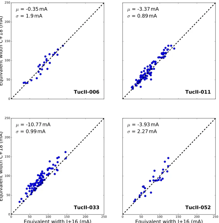
discrepancy(TucII-033), we thus inspected the equivalent width

measurements. After inspecting ﬁts to the individual absorption

lines, it became apparent that the discrepancy is likely due to unfortunate continuum placement issues with the automated

continuumﬁtting routine in previous work. We thus inspected and

compared equivalent widths of all stars, as shown in Figure3. We

ﬁnd a small (somewhat) statistically signiﬁcant difference between measurements for TucII-001 and TucII-052, but which are overall

on the level of 3–4 mÅ, and thus not a source for any signiﬁcant

abundance differences. No offset is found for TucII-006. For

TucII-033, there is indeed a signiﬁcant offset, of ∼10 mÅ, which

indeed explains why we measure systematically increased[Fe/H].

We conclude that any abundance discrepancies are

consis-tent with previous uncertainties, but we now have signiﬁcantly

better S/N than before. Thus, differences in our ﬁnal stellar

parameters and abundances between this work and Ji et al. (2016b) are likely due to the additional observations that we

have combined with theirs for a new analysis presented here.

Walker et al.(2016) measured metallicities for their Tucana II

stars by matching their observed spectra of the Mg b region (∼5150 Å) to a grid of synthetic spectra in the Segue Stellar

Parameters Pipeline(Lee et al.2008). They obtained R∼18,000

spectra of their brighter targets and R∼10,000 of their fainter

targets. Weﬁnd that our metallicities are typically much lower (at

least∼0.50 dex) than those in Walker et al. (2016) for the ﬁve

stars in common, including the four stars in Ji et al.(2016b). There

is no obvious signiﬁcant systematic difference between other

stellar parameters that could explain this offset. We do measure

lower Teffvalues by 70 K on average, but this difference does not

explain such a large difference in the metallicities. Neither do we see trends in our measured Mg abundances that could affect the Mg b region, and consequently, the metallicity measurements in

Walker et al.(2016). Much of the discrepancy, however, can be

attributed to the fact that Walker et al.(2016) applied a metallicity

offset of 0.32 dex to their measurements based on an offset with respect to the measured metallicity of a solar spectrum, which may not be appropriate in our case, given that the Sun and these dwarf galaxy stars have very different stellar parameters.

4. Chemical Signatures of the Tucana II Stellar Population

We ﬁrst explore the possibility that TucII-033 is a halo

interloper in Section 4.1. Then, we discuss the trends of

element abundances provided, and how they characterize the stellar population of Tucana II in the remainder of this section.

Table 3 (Continued)

El. N logò(X)e [X/H] [X/Fe] σa El. N logò(X)e [X/H] [X/Fe] σa

TucII-206 CH 2 8.43 −2.87 0.47 0.28 CHb ₂ _8.43 _−2.61 _0.73 _0.28 NaI 2 6.24 −2.72 0.62 0.46 MgI 3 7.60 −2.89 0.45 0.28 AlI 2 6.45 −3.96:c _−0.62:c _L SiI 1 7.51 −3.14:c _0.20:c _L CaI 2 6.34 −3.08 0.26 0.32 ScII 5 3.15 −3.09 0.25 0.28 TiII 9 4.95 −3.07 0.27 0.28 CrI 3 5.64 −3.46 −0.12 0.28 MnI 3 5.43 −3.81 −0.47 0.28 FeI 46 7.50 −3.34 0.00 0.28 FeII 3 7.50 −3.33 0.01 0.34 SrII 2 2.87 −4.64 −1.30 0.28 BaII 1 2.18 −4.19 −0.85 0.28 EuI 1 0.52 <−2.04 <1.30 L Notes. a

Random uncertainties. See Table4for total uncertainties.

b

Corrected for the evolutionary status of the star following Placco et al.(2014).

c

Colons(:) indicate large uncertainties despite the detection of a line feature. (This table is available in machine-readable form.)

(8)

4.1. Is TucII-033 a Member of Tucana II?

Traditionally, the membership status of stars in dwarf galaxies is derived from a combination of velocity and metallicity measurements. However, the detailed chemical abundances of candidate member stars might also be used to determine membership because UFDs are expected to show distinct

chemical signatures(e.g., lower Fe, Sr, Ba) compared with the

halo background. Additional evidence for non-membership might be gained if any star has chemical abundances distinct from those of other stars in the sample. The small number of stars currently known in UFDs that do not necessarily yield

well-deﬁned abundance trends over large parameter space (e.g.,

[Fe/H]) requires, in particular, that any claim of chemical (non-) membership be investigated thoroughly. Thus, in this section we discuss if any stars in our sample have chemical signatures that challenge their radial velocity membership status.

All stars in our sample except one have abundances that are consistent with those of typical UFD stars, as can be seen in

Figures 4–6. The exception is TucII-033, the most metal-rich

([Fe/H]=−2.41) star. It displays a Sr abundance ([Sr/Fe]= −0.39, [Sr/H]=−2.8) that is in disagreement with that of the

typical UFD stars(Frebel et al.2010b,2014) and, importantly,

with that of the other stars in Tucana II. TucII-033 has a[Sr/H]

abundance distinctly different by 1.7 dex (a 50 fold increase)

from ﬁve of the stars in Tucana II, which have an average

[Sr/H]=−4.46 (with a standard deviation of only 0.14 dex).

The remaining star(TucII-078) is also distinct in that it has a

low upper limit on its Sr abundance. The lack of Sr in TucII-078 relative to the other Tucana II members is puzzling, but

similar stars are known to exist in other UFDs(e.g., Segue I).

TucII-033 has an enhancement in Sr that appears to agree with

the trend for halo stars as shown in Figure6, whereas

TucII-078 and the other Tuc II members have Sr abundances far below the halo trend. This comparison raises the possibility that TucII-033 might be an interloping halo star with the same systemic velocity as TucII.

To further investigate, we determined whether it was plausible for a halo star to have the same systemic velocity

of Tucana II(vsys=−129.1 km s−1; Walker et al. 2016). We

retrieved the velocities of halo stars with metallicities of

[Fe/H]<−2.0 in the literature (Abohalima & Frebel 2017).

Weﬁnd that this sample of 799 halo stars has a distribution of

Table 4 Uncertainties

El. N σrand σsys σtot El. N σrand σsys σtot

TucII-006 TucII-011 CH 2 0.27 0.51 0.58 CH 2 0.31 0.39 0.50 NaI 2 0.27 0.39 0.47 NaI 2 0.23 0.33 0.40 MgI 2 0.37 0.32 0.49 MgI 5 0.16 0.24 0.29 AlI 1 L L L AlI 2 L L L SiI 1 L L L SiI 2 L L L CaI 2 0.27 0.30 0.40 CaI 10 0.21 0.16 0.26 ScII 5 0.27 0.28 0.39 ScII 6 0.16 0.15 0.22 TiII 12 0.27 0.64 0.69 TiI 2 0.16 0.20 0.26 CrI 3 0.27 0.53 0.59 TiII 17 0.22 0.23 0.32 MnI 3 0.27 0.29 0.40 CrI 5 0.20 0.29 0.35 FeI 52 0.27 0.28 0.39 MnI 3 0.17 0.22 0.28 FeII 3 0.27 0.20 0.34 FeI 99 0.16 0.23 0.28 CoI 1 0.34 0.57 0.67 FeII 11 0.16 0.20 0.26 NiI 2 0.66 0.45 0.80 CoI 3 0.21 0.25 0.33 SrII 2 0.27 0.22 0.35 NiI 3 0.22 0.29 0.36 BaII 2 0.27 0.26 0.37 SrII 2 0.19 0.21 0.28 EuI 1 L L L BaII 1 0.20 0.20 0.28 EuI 1 L L L TucII-033 TucII-052 CH 2 0.18 0.41 0.45 CH 2 0.20 0.43 0.47 NaI 2 0.12 0.27 0.30 NaI 2 0.29 0.27 0.40 MgI 4 0.12 0.25 0.28 MgI 2 0.20 0.33 0.39 AlI 2 L L L AlI 1 L L L SiI 2 L L L SiI 2 L L L CaI 8 0.12 0.14 0.18 CaI 4 0.20 0.17 0.26 ScII 5 0.12 0.20 0.23 ScII 5 0.20 0.16 0.26 TiI 2 0.51 0.22 0.56 TiII 12 0.25 0.19 0.31 TiII 12 0.27 0.21 0.34 CrI 5 0.20 0.28 0.34 CrII 1 0.32 0.18 0.36 MnI 4 0.21 0.22 0.30 CrI 5 0.12 0.28 0.30 FeI 56 0.20 0.28 0.34 MnI 3 0.30 0.31 0.43 FeII 3 0.20 0.14 0.24 FeI 92 0.12 0.23 0.26 CoI 3 0.20 0.28 0.34 FeII 12 0.14 0.18 0.23 NiI 2 0.20 0.28 0.34 CoI 2 0.26 0.30 0.40 SrII 2 0.20 0.23 0.30 SrII 2 0.26 0.19 0.32 BaII 2 0.20 0.19 0.28 BaII 2 0.39 0.16 0.42 EuI 1 0.20 0.16 0.26 EuI 1 L L L TucII-078 TucII-203 CH 2 0.20 0.39 0.44 CH 2 0.20 0.43 0.47 NaI 2 0.20 0.21 0.29 NaI 2 0.26 0.24 0.35 MgI 5 0.20 0.25 0.32 MgI 2 0.20 0.29 0.35 AlI 2 L L L AlI 2 L L L SiI 2 L L L SiI 1 L L L CaI 8 0.20 0.15 0.25 CaI 4 0.20 0.19 0.28 ScII 6 0.20 0.23 0.30 ScII 5 0.20 0.20 0.28 TiI 1 0.36 0.25 0.44 TiII 14 0.28 0.17 0.33 TiII 20 0.25 0.25 0.35 VII 1 0.21 0.13 0.25 CrI 5 0.26 0.28 0.38 CrI 3 0.20 0.29 0.35 MnI 2 0.20 0.28 0.34 MnI 3 0.20 0.28 0.34 FeI 83 0.20 0.23 0.30 FeI 59 0.20 0.25 0.32 FeII 9 0.20 0.25 0.32 FeII 4 0.20 0.13 0.24 CoI 1 0.42 0.29 0.51 CoI 2 0.20 0.25 0.32 NiI 2 0.24 0.27 0.36 NiI 3 0.20 0.27 0.34 SrII 1 L L L SrII 1 0.30 0.22 0.37 BaII 1 L L L BaII 1 0.20 0.18 0.27 EuI 1 L L L EuI 1 L L L TucII-206 CH 2 0.28 0.51 0.58 NaI 2 0.46 0.32 0.56 Table 4 (Continued)

El. N σrand σsys σtot El. N σrand σsys σtot

MgI 3 0.28 0.31 0.42 AlI 2 L L L SiI 1 L L L CaI 2 0.32 0.27 0.42 ScII 5 0.28 0.26 0.38 TiII 9 0.28 0.29 0.40 CrI 3 0.28 0.29 0.40 MnI 3 0.28 0.24 0.37 FeI 46 0.28 0.27 0.39 FeII 3 0.34 0.29 0.45 SrII 2 0.28 0.25 0.38 BaII 1 0.28 0.29 0.40 EuI 1 L L L

(9)

velocities that is roughly Gaussian and centered on 15 km s−1

with a standard deviation of 154 km s−1. Using this distribution

of velocities, we can calculate the odds of ﬁnding an

interloping halo star around the mean systemic velocity of

Tucana II. We derive a 6% chance ofﬁnding a halo star within

two times the velocity dispersion (8.6 km s−1 in Walker

et al. 2016) around the mean velocity of Tucana II, and a 9%

chance if we increase the bounds to three times the velocity dispersion. Thus, it is unlikely, but not unreasonable, for a metal-poor halo star to have the same systemic velocity as Tucana II. As an aside, we do note that considering exclusion from our sample likely does not affect the status of Tucana II

as a dwarf galaxy. Walker et al. (2016) measure a mean

velocity for Tucana II of -129_-+3.53.5km s−1 and a velocity

dispersion of 8.6_-+2.7

4.4_{km s}−1_{. The velocity measurement of}

TucII-033(vhelio=−127.5 km s−1) is close to 1σ of the error

on the measured systemic velocity of Tucana II. Thus, it is unlikely that the exclusion of this star would remove any velocity spread that is used to classify Tucana II as a UFD.

While there are also stars in Reticulum II(Ji et al.2016c), a

star in Tucana III (Hansen et al. 2017), and a star in Canes

Venatici II(François et al.2016) that show an enhancement in

Sr, we do not consider them to be typical UFD stars. In the case of Reticulum II and Tucana III, this Sr enhancement is

reﬂective of strong and moderate r-process enrichments,

respectively. Given that the origin of these enhancements clearly derive from r-process events that occurred in these systems, and that these events are regarded rare, we do not consider them to be typical examples of UFDs. Moreover,

TucII-033 is not a r-process enhanced star. It is difﬁcult to

judge the signiﬁcance of the one available Sr abundance

([Sr/Fe]=1.32) in Canes Venatici II. This star has a Sr enhancement that could be a result of a weak r-process

enrichment event(e.g., Wanajo2013) and, in theory, a similar

event may have enhanced TucII-033. However, more data from

Canes Venatici II is needed to deriveﬁrm conclusions. Thus,

around the metallicity of TucII-033 ([Fe/H]∼−2.5), the

typical UFD stellar population either has extremely low upper

limits on the Sr abundance (i.e., Segue 1; [Sr/H]−4.0) or

marginal detections(e.g., stars in Coma Berenices, Ursa Major

II; Frebel et al. 2010b,2014).

This high Sr abundance measurement of TucII-033 also naturally raises the question of why the Sr abundance was not recognized as such in the previous study of this galaxy. Upon

investigation, weﬁnd that we measure a higher Sr abundance

than Ji et al.(2016b) by 0.70 dex. However, their Sr abundance

has a large uncertainty(∼0.6 dex) and somewhat distorted lines

due to low S/N at the Sr lines (407 and 4215 Å). Our improved

S/N in this region clearly shows that high Sr is required.

We do note that TucII-033 is distinct from halo stars in that it

has a markedly lower[α/Fe] ratio (∼0.05 dex) than other halo

stars (∼0.4 dex) as discussed in Section 4.3. Using the

compilation by Abohalima & Frebel(2017), we ﬁnd that only

8% of halo stars have a lower Ca abundance than TucII-033 and 15% have a lower Mg abundance. These fractions, when viewed in the context that TucII-033 has the same systemic velocity as Tucana II, make it less likely that TucII-033 is an interloping star.

For these reasons, for the remainder of the analysis, we present two lines of argument: one assuming TucII-033 as a member, and one assuming TucII-033 as a non-member. The exclusion of TucII-033 from the interpretation of this galaxy

would be meaningful, since its low [α/Fe] abundance would

otherwise imply that Tucana II had an extended star formation

history and would thus not be a surviving ﬁrst galaxy (see

Sections 4.3 and 4.5). While the Sr abundance of TucII-033

might suggest that it is a halo interloper, its[α/Fe] and velocity

make this scenario less likely.

4.2. Carbon

Empirically, a high fraction of EMP stars in the halo(∼42%;

Placco et al.2014) are enhanced in carbon ([C/Fe]>0.7 dex)

and are thus classiﬁed as carbon-enhanced metal-poor stars.

This enhancement in carbon has been used to constrain potential sites of nucleosynthesis that may have dominated

early chemical evolution(e.g., Tominaga et al.2007; Cooke &

Madau 2014; Frebel & Norris 2015). From the paradigm of

hierarchical galaxy formation, we might expect that stars in dwarf galaxies also display this enhancement given that accreted analogs perhaps contributed to the metal-poor population of the halo. However, recent studies of the prevalence of carbon-rich stars in dwarf galaxies give differing

results (Kirby et al. 2015; Jablonka et al. 2015; Chiti

et al.2018).

In Tucana II, we ﬁnd that three stars out of ﬁve with

<

-[Fe H] 2.9 are enhanced in carbon, following the

correction in Placco et al. (2014). This fraction is slightly

larger than that of the halo, with the caveat of the small size of

our sample. One star(TucII-011) appears to be somewhat less

enhanced in carbon ([C/Fe]=0.29 after correction for the

evolutionary state of the star). This slight outlier might reﬂect

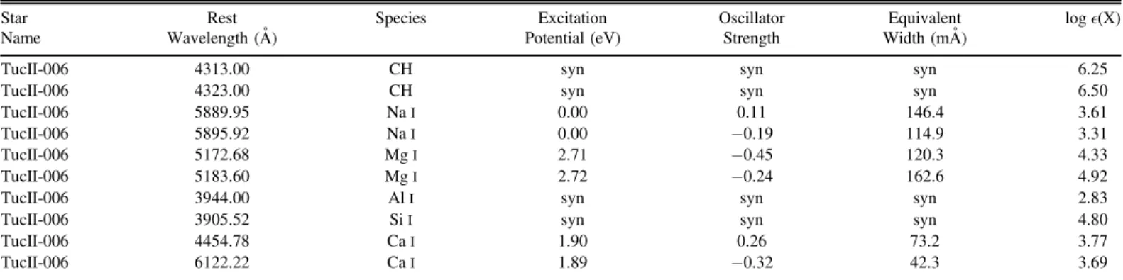
Table 5 Line Measurements

Star Rest Species Excitation Oscillator Equivalent logò(X)

Name Wavelength(Å) Potential(eV) Strength Width(mÅ)

TucII-006 4313.00 CH syn syn syn 6.25

TucII-006 4323.00 CH syn syn syn 6.50

TucII-006 5889.95 NaI 0.00 0.11 146.4 3.61

TucII-006 5895.92 NaI 0.00 −0.19 114.9 3.31

TucII-006 5172.68 MgI 2.71 −0.45 120.3 4.33

TucII-006 5183.60 MgI 2.72 −0.24 162.6 4.92

TucII-006 3944.00 AlI syn syn syn 2.83

TucII-006 3905.52 SiI syn syn syn 4.80

TucII-006 4454.78 CaI 1.90 0.26 73.2 3.77

TucII-006 6122.22 CaI 1.89 −0.32 42.3 3.69

(10)

inhomogeneous mixing of gas in the system or multiple avenues of enrichment that contributed to the chemical evolution of the system.

4.3.α-Elements

The abundance ofα-elements (Mg, Si, Ca, Ti) in stars can be

used investigate the integrated supernovae (SNe) population

that chemically enriched the natal gas cloud of the stars. In

particular, enrichment by core-collapse SNe results in a ﬂat

[α/Fe]∼0.4 trend versus [Fe/H], whereas Type Ia SNe

enrichment result in a declining[α/Fe] abundance trend versus

[Fe/H] (e.g., Iwamoto et al. 1999; Kirby et al. 2011).

Typically, this switch from aﬂat to a declining [α/Fe] versus

[Fe/H] indicates the metallicity at which type Ia SNe started dominating the Fe production. The most metal-rich member

of our sample, TucII-033, shows a slight deﬁciency in its

α-element abundance compared to the other stars in our

sample. This deﬁciency suggests that Type Ia SNe contributed

to the chemical abundances of at least some stars in this galaxy, which in turn would suggest somewhat extended star formation

and chemical enrichment in Tucana II(e.g., Kirby et al.2011).

Declining [α/Fe] is seen in most UFDs (Vargas et al.2013),

though Tucana II is one of the least luminous UFDs with

available[α/Fe] measurements.

If TucII-033 were a halo interloper (see Section 4.1), our

sample would instead show a trend consistent with a constant

Figure 3.Comparison of the equivalent widths of FeIlines measured on the same spectra using our method and Ji et al.(2016b). The mean offset and standard error

(11)

[α/Fe], as produced by core-collapse SNe only. We note, that the lower Mg abundance displayed by TucII-006 is likely due to a distortion in one of the two lines used to measure its

abundance, which is reﬂected in the larger uncertainties on its

Mg abundance of 0.46 dex.

4.4. Odd-Z, Iron-peak, and Neutron-capture Element Abundances

Weﬁnd no signiﬁcant deviation from the halo trend in the

odd-Z elements (Na, Al, Sc) and iron-peak elements (Cr, Mn,

Co, Ni). This is also consistent with abundances of other UFD

stars in the literature(see Figures4and5). We do ﬁnd one star

(TucII-078) with a lower Na abundance than typical halo and dwarf galaxy stars.

We ﬁnd low strontium and barium abundances in six stars

that are characteristic of the stellar populations set by other

UFD stars (see Figure6). See Section 4.1for a discussion of

the neutron-capture element abundances in TucII-033. We do

not detect europium or other neutron-capture elements in any stars in our sample.

4.5. Tucana II As a Surviving First Galaxy

Frebel & Bromm(2012) predict chemical characteristics of

the population of survivingﬁrst galaxies:

1. a large spread in[Fe/H] (∼1 dex);

2. light element abundance ratios in agreement with a core-collapse supernova enrichment;

3. no stars with[α/Fe] systemically lower than the galactic

halo abundance of[α/Fe]∼0.35; and

4. no signatures of s-process enhancement from AGB stars.

The ﬁrst prediction is a consequence of inhomogeneous

mixing in the ﬁrst galaxies, and the last two predictions are

consequences of theﬁrst galaxies being enriched by “one-shot”

chemical enrichment events as extended star formation is not

thought to have occurred in the ﬁrst galaxies. The second

Figure 4.[X/Fe] vs. [Fe/H] ratio for the abundances of carbon, the odd-Z elements, the iron-peak elements, and europium. Gray data points correspond to stars in the halo (Frebel2010; Roederer et al. 2014). Colored symbols are UFD stars. Error bars correspond to random uncertainties; see Table4for total uncertainties. Abundances marked by colons(:) in Table3are shown with uncertainties of 0.5 dex. The carbon abundances in this plot are not corrected for the evolutionary state of each star following(Placco et al.2014); see Table3for corrected carbon abundances. In general, the abundances of these elements in Tucana II stars agree with trends in other UFDs and the Milky Way halo. UFD abundances are from Koch et al.(2008), Feltzing et al. (2009), Frebel et al. (2010a,2010b,2014), Norris et al. (2010a,

2010b), Simon et al. (2010), Gilmore et al. (2013), Koch et al. (2013), Ishigaki et al. (2014), Koch & Rich (2014), Roederer & Kirby (2014), Ji et al. (2016b,2016c,

(12)

criterion simply conﬁrms enrichment by supernovae. Accord-ing to our chemical abundance results, Tucana II largely

satisﬁes the aforementioned ﬁrst, second, and fourth criteria for

a survivingﬁrst galaxy. The second one would also be satisﬁed

if we exclude TucII-033 when assuming it is a halo interloper

(see Section 4.1). However, if we include TucII-033 in the

interpretation, then its Sr relative enhancement relative to other

Tuc II members and[α/Fe] deﬁciency would imply that Tuc II

had undergone some period of chemical evolution, and would

thus not be a surviving ﬁrst galaxy. Given the low luminosity

of Tucana II(~ ´3 103L;Bechtol et al.2015; Koposov et al.

2015), it would still be interesting to ﬁnd that Tucana II has

some chemical evolution as opposed to isolated chemical enrichment events.

Together with Segue 1(Frebel et al.2014), Tucana II might

still be one of the best candidates for a survivingﬁrst galaxy, as

determined from chemical abundances of six stars in each galaxy. Moreover, these six stars form the majority of known members in Tucana II, and their chemical abundances suggest that most stars in the galaxy are consistent with having formed

in an environment similar to a ﬁrst galaxy. Theoretical

modeling of early galaxies such as these two systems could shed further light on this issue. However, detailed abundances

of more stars with[Fe/H]−2.5 in Tucana II are needed to

further investigate the nature and origin of Tucana II, as is the

case with other potential ﬁrst galaxy candidates (i.e., Ursa

Major II, Coma Berenices, Leo IV).

5. Conclusion

In this paper, we presented the high-resolution chemical abundance measurements of seven stars in the Tucana II dwarf galaxy. Three stars with no previous high-resolution chemical abundance measurements were analyzed. Four other stars had

been reanalyzed from the sample in Ji et al. (2016b) with the

addition of new data.

From the detection of new members and the reanalysis of known members, we were able to discuss the chemical signatures of stars in the Tucana II UFD. We raise the

possibility that one of the stars (TucII-033) may be an

interloping halo star given its high Sr abundance with respect

to other known UFD stars, but its velocity and [α/Fe] ratio

make this unlikely. Excluding TucII-033 from the

interpreta-tion, Tucana II does meet all the criteria to be a survivingﬁrst

galaxy (Frebel & Bromm 2012). Assuming TucII-033 is a

member, Tucana II would not meet the one-shot enrichment

criterion due to the star’s low [α/Fe] and likely somewhat

extended chemical evolution.

We conﬁrmed two new members of Tucana II that were

pre-selected as probable members from SkyMapper

photo-metry. Given the large ﬁeld of view of the SkyMapper

telescope(5.7 sq. deg.) and the metallicity discriminating “v”

ﬁlter, we were able to search for metal-poor stars within a large area around TucII UFD. As a result, our two new

members are∼2 half-light radii from the center of Tucana II

and may have been missed by traditional spectroscopic

follow-up observations (see Figure 2). Interestingly, one of

these new members is the most metal-poor star discovered in

Tucana II thus far ([Fe/H]=−3.34). From our small

sample, we cannot, however, claim these new members display systematic differences to stars near the center of Tucana II.

This new photometric metal-poor star identiﬁcation

techni-que might aid in identifying members for detailed chemical analysis and studying potential correlations with substructure of UFD systems. Combining this photometric selection technique with traditional spectroscopic follow-up would result

in more accurate parameters for UFDs (e.g., half-light radii,

mass-to-light ratios), supposing the photometry itself could

predict membership status. In particular, this highly efﬁcient

large ﬁeld of view method for ﬁnding members would be

interesting to apply on systems that show potential elongated

Figure 5.[X/Fe] vs. [Fe/H] ratio of abundances of α-element abundances in stars in Tucana II. Gray data points correspond to stars in the halo (Frebel2010; Roederer et al.2014). Colored symbols are UFD stars. Error bars correspond to random uncertainties; see Table4for total uncertainties. Abundances marked by colons(:) in Table3are shown with uncertainties of 0.5 dex. The decrease in the[α/Fe] ratio of the most metal-rich star (TucII-033) would suggest that Tucana II had an extended star formation history, but see Section4.1for a discussion on the membership of TucII-033.

(13)

tidal features, such as Tucana III (Drlica-Wagner et al. 2016;

Simon et al.2017). Moreover, the spectroscopic study of more

stars in UFDs would have multiple beneﬁts. For instance,

detecting more stars with [Fe/H]∼−2.5 in Tuc II would

potentially resolve whether the entire galaxy had undergone chemical evolution. This would better inform whether TucII-033 is indeed a halo interloper or rather signaling unusual enrichment events or some degree of chemical evolution in that UFD. At minimum, future work will extend this selection

technique to other UFDs for the purpose of efﬁciently

identifying new members and enabling detailed abundance measurements.

We thank Dougal Mackey and Christian Wolf for helpful comments on reducing the SkyMapper photometry. A.C. and A.F. are supported by NSF CAREER grant AST-1255160. A.F. acknowledges partial support from PHY 14-30152; and

Physics Frontier Center/JINA Center for the Evolution of the

Elements (JINA-CEE), awarded by the US National Science

Foundation. A.P.J. is supported by NASA through Hubble Fellowship grant HST-HF2-51393.001 awarded by the Space Telescope Science Institute, which is operated by the Associa-tion of Universities for Research in Astronomy, Inc., for NASA, under contract NAS5-26555. H.J. and J.E.N. acknowl-edge the support of the Australian Research Council through

Figure 6.[X/Fe] vs. [Fe/H] and [X/H] vs. [Fe/H] ratio of abundances of strontium and barium in stars in Tucana II. Gray data points correspond to stars in the halo (Frebel2010; Roederer et al.2014). Colored symbols are UFD stars. Error bars correspond to random uncertainties; see Table4for total uncertainties and Section3.1

for a discussion on deriving uncertainties. The most metal-rich star in Tucana II(TucII-033) has Sr and Ba abundances that are above those typically seen in UFD stars.

(14)

Discovery project DP150100862. The national facility cap-ability for SkyMapper has been funded through ARC LIEF grant LE130100104 from the Australian Research Council, awarded to the University of Sydney, the Australian National University, Swinburne University of Technology, the Uni-versity of Queensland, the UniUni-versity of Western Australia, the University of Melbourne, Curtin University of Technology, Monash University and the Australian Astronomical Observa-tory. SkyMapper is owned and operated by The Australian

National University’s Research School of Astronomy and

Astrophysics. This work made use of NASAs Astrophysics Data System Bibliographic Services. This work has also made

extensive use of the astropy package (Astropy Collaboration

et al.2013).

Facilities: Magellan:Clay (MIKE), SkyMapper.

Software: Turbospectrum(Alvarez & Plez1998; Plez2012),

MARCS(Gustafsson et al.2008), MIKE CarPy (Kelson2003),

MOOG (Sneden 1973), Astropy (Astropy Collaboration et al.

2013).

ORCID iDs

Anirudh Chiti https://orcid.org/0000-0002-7155-679X

Anna Frebel https://orcid.org/0000-0002-2139-7145

Helmut Jerjen https://orcid.org/0000-0003-4624-9592

John E. Norris https://orcid.org/0000-0002-7900-5554

References

Abohalima, A., & Frebel, A. 2017, ApJS, in press(arXiv:1711.04410)

Alvarez, R., & Plez, B. 1998, A&A,330, 1109

Asplund, M., Grevesse, N., Sauval, A. J., & Scott, P. 2009,ARA&A,47, 481

Bechtol, K., Drlica-Wagner, A., Balbinot, E., et al. 2015,ApJ,807, 50

Beers, T. C., & Christlieb, N. 2005,ARA&A,43, 531

Belokurov, V. 2013,NewAR,57, 100

Belokurov, V., Zucker, D. B., Evans, N. W., et al. 2007,ApJ,654, 897

Bernstein, R., Shectman, S. A., Gunnels, S. M., Mochnacki, S., & Athey, A. E 2003,Proc. SPIE,4841, 1694

Bessell, M., Bloxham, G., Schmidt, B., et al. 2011,PASP,123, 789

Bessell, M., & Murphy, S. 2012,PASP,124, 140

Bromm, V., Yoshida, N., Hernquist, L., & McKee, C. F. 2009,Natur,459, 49

Brown, T. M., Tumlinson, J., Geha, M., et al. 2014,ApJ,796, 91

Casagrande, L., & VandenBerg, D. A. 2014,MNRAS,444, 392

Casey, A. R. 2014, PhD thesis, Australian National Univ. Castelli, F., & Kurucz, R. L. 2004, arXiv:astro-ph/0405087

Chiti, A., Simon, J. D., Frebel, A., et al. 2018,ApJ,856, 142

Cooke, R. J., & Madau, P. 2014,ApJ,791, 116

Den Hartog, E. A., Lawler, J. E., Sneden, C., & Cowan, J. J. 2003,ApJS,

148, 543

Dotter, A., Chaboyer, B., Jevremović, D., et al. 2008,ApJS,178, 89

Drlica-Wagner, A., Bechtol, K., Allam, S., et al. 2016,ApJL,833, L5

Drlica-Wagner, A., Bechtol, K., Rykoff, E. S., et al. 2015,ApJ,813, 109

Feltzing, S., Eriksson, K., Kleyna, J., & Wilkinson, M. I. 2009,A&A,508, L1

François, P., Monaco, L., Bonifacio, P., et al. 2016,A&A,588, A7

Frebel, A. 2010,AN,331, 474

Frebel, A., & Bromm, V. 2012,ApJ,759, 115

Frebel, A., Casey, A. R., Jacobson, H. R., & Yu, Q. 2013,ApJ,769, 57

Frebel, A., Christlieb, N., Norris, J. E., et al. 2007,ApJL,660, L117

Frebel, A., Kirby, E. N., & Simon, J. D. 2010a,Natur,464, 72

Frebel, A., & Norris, J. E. 2013, in Planets, Stars, and Stellar Systems, Vol. 5, ed. T. Oswalt & G. Gilmore(Dordrecht: Springer),55

Frebel, A., & Norris, J. E. 2015,ARA&A,53, 631

Frebel, A., Simon, J. D., Geha, M., & Willman, B. 2010b,ApJ,708, 560

Frebel, A., Simon, J. D., & Kirby, E. N. 2014,ApJ,786, 74

Freeman, K., & Bland-Hawthorn, J. 2002,ARA&A,40, 487

Gilmore, G., Norris, J. E., Monaco, L., et al. 2013,ApJ,763, 61

Gustafsson, B., Edvardsson, B., Eriksson, K., et al. 2008,A&A,486, 951

Hansen, T. T., Simon, J. D., Marshall, J. L., et al. 2017,ApJ,838, 44

Heger, A., & Woosley, S. E. 2010,ApJ,724, 341

Hill, V., Plez, B., Cayrel, R., et al. 2002,A&A,387, 560

Homma, D., Chiba, M., Okamoto, S., et al. 2016,ApJ,832, 21

Homma, D., Chiba, M., Okamoto, S., et al. 2018,PASJ,70, S18

Ishigaki, M. N., Aoki, W., Arimoto, N., & Okamoto, S. 2014, A&A,

562, A146

Ivans, I. I., Simmerer, J., Sneden, C., et al. 2006,ApJ,645, 613

Iwamoto, K., Brachwitz, F., Nomoto, K., et al. 1999,ApJS,125, 439

Jablonka, P., North, P., Mashonkina, L., et al. 2015,A&A,583, A67

Ji, A. P., Frebel, A., Chiti, A., & Simon, J. D. 2016a,Natur,531, 610

Ji, A. P., Frebel, A., Ezzeddine, R., & Casey, A. R. 2016b,ApJL,832, L3

Ji, A. P., Frebel, A., Simon, J. D., & Chiti, A. 2016c,ApJ,830, 93

Ji, A. P., Frebel, A., Simon, J. D., & Geha, M. 2016d,ApJ,817, 41

Karlsson, T., Bromm, V., & Bland-Hawthorn, J. 2013,RvMP,85, 809

Kelson, D. D. 2003,PASP,115, 688

Kenney, J. F. 1962, Mathematics of Statistics (3rd ed; Princeton, NJ: Van Nostrand)

Kim, D., & Jerjen, H. 2015,ApJL,808, L39

Kim, D., Jerjen, H., Mackey, D., Da Costa, G. S., & Milone, A. P. 2015,ApJL,

804, L44

Kirby, E. N., Cohen, J. G., Guhathakurta, P., et al. 2013,ApJ,779, 102

Kirby, E. N., Cohen, J. G., Simon, J. D., et al. 2017,ApJ,838, 83

Kirby, E. N., Cohen, J. G., Smith, G. H., et al. 2011,ApJ,727, 79

Kirby, E. N., Guo, M., Zhang, A. J., et al. 2015,ApJ,801, 125

Koch, A., Feltzing, S., Adén, D., & Matteucci, F. 2013,A&A,554, A5

Koch, A., McWilliam, A., Grebel, E. K., Zucker, D. B., & Belokurov, V. 2008,

ApJL,688, L13

Koch, A., & Rich, R. M. 2014,ApJ,794, 89

Koposov, S. E., Belokurov, V., Torrealba, G., & Evans, N. W. 2015,ApJ,

805, 130

Laevens, B. P. M., Martin, N. F., Bernard, E. J., et al. 2015a,ApJ,813, 44

Laevens, B. P. M., Martin, N. F., Ibata, R. A., et al. 2015b,ApJL,802, L18

Lawler, J. E., Den Hartog, E. A., Sneden, C., & Cowan, J. J. 2006,ApJS,

162, 227

Lawler, J. E., Sneden, C., Cowan, J. J., Ivans, I. I., & Den Hartog, E. A. 2009,

ApJS,182, 51

Lee, Y. S., Beers, T. C., Sivarani, T., et al. 2008,AJ,136, 2022

Martin, N. F., de Jong, J. T. A., & Rix, H.-W. 2008,ApJ,684, 1075

Masseron, T., Plez, B., Van Eck, S., et al. 2014,A&A,571, A47

Nagasawa, D. Q., Marshall, J. L., Li, T. S., et al. 2018,ApJ,852, 99

Norris, J. E., Gilmore, G., Wyse, R. F. G., Yong, D., & Frebel, A. 2010a,

ApJL,722, L104

Norris, J. E., Yong, D., Gilmore, G., & Wyse, R. F. G. 2010b,ApJ,711, 350

Piskunov, N. E., Kupka, F., Ryabchikova, T. A., Weiss, W. W., & Jeffery, C. S. 1995, A&AS,112, 525

Placco, V. M., Frebel, A., Beers, T. C., & Stancliffe, R. J. 2014,ApJ,797, 21

Plez, B. 2012, Turbospectrum: Code for spectral synthesis, Astrophysics Source Code Library, ascl:1205.004

Astropy Collaboration, Robitaille, T. P, Tollerud, E. J, et al. 2013, A&A,

558, A33

Roederer, I. U., & Kirby, E. N. 2014,MNRAS,440, 2665

Roederer, I. U., Preston, G. W., Thompson, I. B., et al. 2014,AJ,147, 136

Ryabchikova, T., Piskunov, N., Kurucz, R. L., et al. 2015,PhyS,90, 054005

Simon, J. D., Frebel, A., McWilliam, A., Kirby, E. N., & Thompson, I. B. 2010,ApJ,716, 446

Simon, J. D., & Geha, M. 2007,ApJ,670, 313

Simon, J. D., Li, T. S., Drlica-Wagner, A., et al. 2017,ApJ,838, 11

Sneden, C., Lawler, J. E., Cowan, J. J., Ivans, I. I., & Den Hartog, E. A. 2009,

ApJS,182, 80

Sneden, C., McWilliam, A., Preston, G. W., et al. 1996,ApJ,467, 819

Sneden, C. A. 1973, PhD thesis, Univ. Texas

Sobeck, J. S., Kraft, R. P., Sneden, C., et al. 2011,AJ,141, 175

Spite, F., & Spite, M. 1982, A&A,115, 357

Starkenburg, E., Martin, N., Youakim, K., et al. 2017,MNRAS,471, 2587

Starkenburg, T. K., & Helmi, A. 2015,A&A,575, A59

Tolstoy, E., Hill, V., & Tosi, M. 2009,ARA&A,47, 371

Tominaga, N., Maeda, K., Umeda, H., et al. 2007,ApJL,657, L77

Vargas, L. C., Geha, M., Kirby, E. N., & Simon, J. D. 2013,ApJ,767, 134

Venn, K. A., Starkenburg, E., Malo, L., Martin, N., & Laevens, B. P. M. 2017,

MNRAS,466, 3741

Walker, M. G., Mateo, M., Olszewski, E. W., et al. 2016,ApJ,819, 53

Walsh, S. M., Jerjen, H., & Willman, B. 2007,ApJL,662, L83

Wanajo, S. 2013,ApJL,770, L22

Willman, B. 2010,AdAst, 2010, 285454

Willman, B., Blanton, M. R., West, A. A., et al. 2005,AJ,129, 2692

(15)

Erratum:

“Chemical Abundances of New Member Stars in the Tucana II Dwarf Galaxy”

(

2018, ApJ, 857, 74

)

Anirudh Chiti1 , Anna Frebel1 , Alexander P. Ji2,5, Helmut Jerjen3 , Dongwon Kim4, and John E. Norris3

1

Department of Physics and Kavli Institute for Astrophysics and Space Research, Massachusetts Institute of Technology, Cambridge, MA 02139, USA;

achiti@mit.edu

2

Observatories of the Carnegie Institution of Washington, 813 Santa Barbara Street, Pasadena, CA 91101, USA

3

Research School of Astronomy and Astrophysics, Australian National University, Canberra, ACT 2611, Australia

4_{Astronomy Department, University of California, Berkeley, CA, USA}

Received 2018 May 9; published 2018 June 14

The coordinates for TucII-078 in Table1and the location of TucII-078 in the right panel of Figure2were incorrect. The correct

coordinates for TucII-078 are now listed in Table1and the correct location of the star is shown in the right panel of Figure2. There

were no other references to the coordinates of this star in the text.

Table 1 Observations

Name R.A.(h:m:s) (J2000) Decl.(d:m:s) (J2000) Slit Size g(mag) texp(minutes) S/Na vhelio(km s−1)

TucII-006 22:51:43.06 −58:32:33.7 1 0 18.78 206b 15, 30 −126.1 TucII-011 22:51:50.28 −58:37:40.2 1 0 18.27 314b _{15, 30} _−124.6 TucII-033 22:51:08.32 −58:33:08.1 1 0 18.68 155b _{17, 32} _−126.9 TucII-052 22:50:51.63 −58:34:32.5 1 0 18.83 155b _{17, 35} _−119.9 TucII-078 22:50:41.07 −58:31:08.3 1 0 18.62 215 15, 30 −123.8 TucII-203 22:50:08.87 −58:29:59.1 1 0 18.81 275 16, 37 −126.1 TucII-206 22:54:36.67 −58:36:57.9 1 0 18.81 385 15, 37 −122.9 Notes. a

S/N per pixel is listed for 4500 and 6500 Å.

b

Combined exposure time from Ji et al.(2016) and this work.

Figure 2.Left: color–magnitude diagram of Tuc II stars from this study. A Dartmouth isochrone (Dotter et al.2008) with an age of 12.5 Gyr, distance modulus of

18.8, and a metallicity of[Fe/H]=−2.5 is overplotted in black along with offsets of (g−r)±0.1 in dashed lines to guide the eye. We denote with different colors the four members previously observed by Ji et al.(2016), one member selected from Walker et al. (2016), and two selected from our SkyMapper photometry. Open circles

indicate conﬁrmed members in Walker et al. (2016) with no high-resolution spectroscopic observations. Right: spatial distribution of Tuc II members centered on the

coordinates of Tucana II. The elliptical half-light radius from Koposov et al.(2015) is overplotted. In both plots, each star is labeled by its identiﬁer as found Table1.

5

(16)