Optimization of Gas Transmission Networks under Energetic and Environmental Considerations

HAL Id: hal-03151331

https://hal.archives-ouvertes.fr/hal-03151331

HAL is a multi-disciplinary open access archive for the deposit and dissemination of sci-entific research documents, whether they are pub-lished or not. The documents may come from teaching and research institutions in France or abroad, or from public or private research centers.

L’archive ouverte pluridisciplinaire HAL, est destinée au dépôt et à la diffusion de documents scientifiques de niveau recherche, publiés ou non, émanant des établissements d’enseignement et de recherche français ou étrangers, des laboratoires publics ou privés.

Optimization of Gas Transmission Networks under

Energetic and Environmental Considerations

Guillermo Hernandez-Rodriguez, Luc Pibouleau, Catherine Azzaro-Pantel,

Serge Domenech

To cite this version:

Guillermo Hernandez-Rodriguez, Luc Pibouleau, Catherine Azzaro-Pantel, Serge Domenech. Opti-mization of Gas Transmission Networks under Energetic and Environmental Considerations. Inter-national Journal of Chemical Reactor Engineering, De Gruyter, 2010, 8 (1), pp.0. �10.2202/1542-6580.2083�. �hal-03151331�

OATAO is an open access repository that collects the work of Toulouse researchers and makes it freely available over the web where possible

Any correspondence concerning this service should be sent

to the repository administrator: tech-oatao@listes-diff.inp-toulouse.fr

This is an author’s version published in: http://oatao.univ-toulouse.fr/27476

To cite this version:

Hernandez-Rodriguez, Guillermo and Pibouleau, Luc and Azzaro-Pantel, Catherine and Domenech, Serge Optimization of Gas Transmission Networks under Energetic and Environmental Considerations. (2010)

International Journal of Chemical Reactor Engineering, 8 (1). ISSN 1542-6580

I

NTERNATIONAL

J

OURNAL OF

C

HEMICAL

R

EACTOR

E

NGINEERING

Volume8 2010 ArticleA136

Optimization of Gas Transmission

Networks under Energetic and

Environmental Considerations

Guillermo Hernandez Rodriguez∗ Luc Guy Pibouleau†

Catherine Azzaro Pantel‡ Serge Domenech∗∗

∗_{Laboratoire de G´enie Chimique, guillermo.hernandez@ensiacet.fr} †_{Laboratoire de G´enie Chimique, luc.pibouleau@ensiacet.fr} ‡_{Laboratoire de G´enie Chimique, catherine.azzarol@ensiacet.fr} ∗∗_{Laboratoire de G´enie Chimique, serge.domenech@ensiacet.fr}

Optimization of Gas Transmission Networks under

Energetic and Environmental Considerations

Guillermo Hernandez Rodriguez, Luc Guy Pibouleau, Catherine Azzaro Pantel, and Serge Domenech

Abstract

The transport of large quantities of natural gas (NG) is carried out by pipeline network systems across long distances. Pipeline network systems include one or several compressor stations which compensate for pressure drops. A typical net-work today might consist of thousands of pipes, dozens of stations, and many other devices, such as valves and regulators. Inside each station, there can be sev-eral groups of compressor units of various vintages that were installed as the ca-pacity of the system expanded. The compressor stations typically consume about 3 to 5% of the transported gas. It is estimated that the global optimization of operations can save considerably the fuel consumed by the stations. Hence, the problem of minimizing fuel cost is of great importance. This study presents a mathematical formulation for NG transport through pipelines and compressors by considering the mass and energy balance equations on the basic elements of a di-dactic network from the literature. First, a deterministic optimization procedure is implemented. The objective of this formulation is the fuel minimization problem in the compressor stations for a fixed gas mass flow delivery. A second example is devoted to the simultaneous consideration of gas mass flow delivery maximization and fuel consumption minimization. In that case, two procedures are compared: a genetic algorithm coupled with a Newton-Raphson procedure and the scalariza-tion method of ?-constraint. In both monobjective and biobjective cases, a study of carbon dioxide (CO2) emissions is carried out. The Pareto front deduced from

the biobjective optimization can be used either for identifying the minimum and maximum network capacity in terms of CO2 emissions and mass flow delivery or

∗_{The authors graciously acknowledge the funding of this work to the Secretaria de Educacio}

Pub-lica (SEC) and the Consejo Nacional de Ciencia y Tecnologia (CONACYT) from the Mexican Government.

for a given mass flow delivery for determining the minimal CO2 emissions from

an appropriate operating of the compressor stations.

KEYWORDS: optimization, pipeline, fuel consumption, natural gas, carbon diox-ide emissions

Introduction

Natural Gas (NG) is an important source of energy for reducing pollution and maintaining a clean and healthy environment. In addition to being a domestically abundant and secure source of energy, the use of NG also offers a number of environmental benefits over other sources of energy, particularly other fossil fuels. The transport of large quantities of NG is carried out by pipeline network systems across long distances. As the gas flows through the network, pressure (and energy) is lost due to both friction between the gas and the pipe inner wall, and heat transfer between the gas and its environment. Typically, NG compressor stations are located at regular intervals along the pipeline to boost the pressure lost through the friction of the NG moving through the steel pipe. They consume a significant part of the transported gas (3 to 5%, Suming et al., 2000), thus resulting in an important fuel consumption cost on the one hand, and in a significant contribution to CO2 emissions, on the other hand. Nowadays, more than 50% of the total human-caused Greenhouse gas (GHG) emissions result from the production and use of energy. About 70% of GHG emissions from NG occur when it is burned to produce heat or energy. Pipelines emit CO2 mainly due to energy used at compression stations. Therefore, pipeline companies reduce GHG emissions mainly by improving the use of energy by acquiring more efficient equipment and by adopting better operating practices (Mora and Ulieru, 2005).

Thus, efficient operation of compressor stations is of major importance for enhancing the performance of the pipeline network. This paper is devoted to the presentation of (1) a gas transportation model taking into account the elements of the network under steady-state conditions that serve for operation condition optimization or design targets and, (2) two approaches for optimizing the performance of compression stations.

In the first part, gas pipeline network modelling provides the ability to represent the behaviour of the system under a variety of conditions, so that it can be used to support optimization procedures. In the second part, a classical deterministic optimization procedure based either on the nonlinear programming tool CONOPT3 of the GAMS (General Algebraic Modelling System) library or on the MATMAB toolbox has been implemented. The objective of this formulation is the fuel minimization problem in the compressor stations for fixed gas mass flow delivery. Then, a genetic algorithm (NSGA IIb, Gomez, 2008) coupled with a Newton-Raphson method and a scalarization procedure based on the -constraint technique are used to solve a biobjective problem, that is the simultaneous maximization of the gas mass flow delivery and the minimization of the fuel consumption in the compression stations. Both monobjective and biobjective optimization procedures are implemented on a didactic network

coming from the literature (Abbaspour et al., 2005), and a study of carbon dioxide emissions by the compression stations is carried out.

Transmission pipeline modelling

Previous works

Since 20 years, there has been an increased interest on the optimization of gas pipe distribution networks. Tian and Adewumi (1994) have proposed a one-dimensional compressible fluid flow equation. Lewandowski (1994) has implemented an object-oriented methodology for modelling a natural gas transmission network, and Osiadacz (1994) has presented a dynamic optimization of high-pressure gas networks. Surry et al. (1995) have formulated the optimization problem based on a multiobjective genetic algorithm. Mohitpour et al. (1996) have used a dynamic simulation approach. Boyd et al. (1997) have studied steady-state gas pipeline networks by modelling the compressor stations. Sung(1998) has based the modelling approach on a hybrid network. Sun et al. (1999) have used a software support system, called the Gas Pipeline Operation Advisor for minimizing the overall operating costs, subject to a set of constraints such as the horsepower requirement, availability of individual compressors, compressor types and cycles. A reduction technique for natural gas transmission network was implemented by Rios-Mercado et al. (2001). Martinez-Romero et al. (2002) have used the software package “Gas Net”. A MINLP model for the problem of minimizing the fuel consumption in a pipeline network was implemented by Cobos-Zaleta and Rios-Mercado (2002). Costa et al. (2002) have developed a steady-state gas pipeline simulation. Mora and Ulieru (2005) have determined the pipeline operation configurations requiring the minimum amount of energy. Chauvelier-Alario et al. (2006) have developed CARPATHE, a simulation package (French Company GdF Suez) for representing the behaviour of multi-pressure networks. Optimization methods for reinforcement planning on gas transportation networks and for minimizing the investment cost of an existing gas transmission network were used by André et al. (2006).

Modelling gas pipeline networks

The objective of this work is to propose a general framework able to embed formulations from design to operational purposes for steady-state problems. The goal is to implement, for a given pipeline network, an accurate numerical method able to be used within an optimization loop. The modelling of gas pipeline networks has already been presented by Tabkhi (2007); only the main points are recalled here.

Gas pipeline equations

The governing equation giving the pressure at each point of a straight pipe can be derived as follows: 0 ) ( 2 2 2 _{ }  v dx d v D f dx dP _{ } (1)

where  is the gas density (kg/m3), D the pipe diameter, v the average gas velocity (m/s).

The Darcy friction factor, f, is a dimensionless value that is a function of the Reynolds number, Re, and relative roughness of the pipeline, /D. The Darcy friction factor is numerically equal to four times of the Fanning friction factor that is preferred by some engineers. Since the regime of the gas passing through pipelines lies in the turbulent range, it is assumed that the wall roughness is the limiting factor compared with the Reynolds number to find out the value of the friction factor. The work of Romeo et al. (2002) is used to estimate the friction factor. The momentum balance in terms of pressure and throughput can be written in the following form:

0 ) ( 16 8 4 2 2 5 2 2    P ZT dx d MD m R P MD m fZRT dx dP     (2)

In this equation, Z is the compressibility factor, R the universal gas constant (8314 J/kmol-°K), T the temperature (°K), M the average molecular mass of the gas, and m the pipe throughput (flow rate in kg/s).

By integrating Eq. (2) between two points i and j, the following equation is obtained and will be used in the numerical formulations:

0 16 ln 32 5 2 2 4 2 2 2 2   _          MD L m fZRT P P MD m ZRT P P j i j i _{ }   ₍₃₎

where L (m) is the pipe length between points i and j.

The compressibility factor, Z, is used to alter the ideal gas equation to account for the real gas behaviour. This factor can be expressed by the following relation: c ij c p p T T Z 1(0.257-0.533 ) (4)





The pseudo-critical temperature of natural gas, Tc, and pseudo-critical pressure, pc, can be calculated using an adequate mixing rule starting from the critical properties of the NG components. In this work, average pseudo-critical properties of the gas are determined from the given mole fractions of its components by Kay’s rule which is a simple linear mixing rule shown in Eq. (5) and (6). Then average pressure, pij, can be calculated from two end pressures (Mohring et al., 2004): ) -( 3 2 j i j i j i ij p p p p p p p    (7)

Maximum allowable operational pressure (MAOP)

The internal pressure in a pipe causes the pipe wall to be stressed, and if it is allowed to reach the yield strength of the pipe material, it could cause permanent deformation of the pipe and ultimate failure. In addition to the internal pressure due to gas flowing through the pipe, the pipe might also be subjected to external pressure which can result from the weight of the soil above the pipe in a buried pipeline, and also by the probable loads transmitted from vehicular traffic. The pressure at all points of the pipeline should be less than the maximum allowable operating pressure (MAOP) which is a design parameter in the pipeline engineering. This upper limit is calculated using Eq. (9), where t is the thickness of the pipe (Menon, 2005):

MAOP p (8) T E F f f f t D t SMYS MAOP -2  (9)

The yield stress used in Eq. (9), is called the specified minimum yield strength (SMYS) of pipe material. SMYS is a mechanical property of the construction material of the gas pipeline. The factor fF is the so-called design factor. This factor is usually 0.72 for cross-country or offshore gas pipelines, but can be as low as 0.4, depending on class location and type of construction. The class location, in turn, depends on the population density in the vicinity of the pipeline. The seam joint factor, fE, varies with the type of pipe material and joint type. Seam joint factors are between 1 and 0.6 for the most commonly used

material types. The temperature factor,fT, is equal to 1 for the gas temperature below 393°K but it can reach 0.867 at 503°K. For each particular problem, these factors are well known by the NG practitioners.

Critical velocities

As flow rate increases due to the augmentation in pressure drop, so does the gas velocity. For a compressible flow, the increase in flow owing to the pressure drop increase is limited to the velocity of sound in the fluid, i.e., the critical velocity. Sonic or critical velocity is the maximum velocity which a compressible fluid can reach in a pipe. For trouble-free operation, velocities maintain under a half of sonic velocity. The sonic velocity in a gas, c is calculated using Eq. (11), where κ is the average isentropic exponent of the gas, and Cp is the heat capacity at constant pressure in J/(kmol.K).

2 / c v (10) M ZRT c  (11) R y C y C i i p i i p  





Increasing gas velocity in a pipeline can have a particular effect on the level of vibration and increase the noises too. The upper limit of the velocity range should be such that erosion-corrosion cavitations or impingement attack will be minimal. The upper limit of the gas velocity for the design purposes is usually computed empirically with the following equation (Menon, 2005). The erosional velocity must always be lower than the speed of sound in the gas.

e v v (13) PM ZRT v_e 122 (14) Compressor characteristics

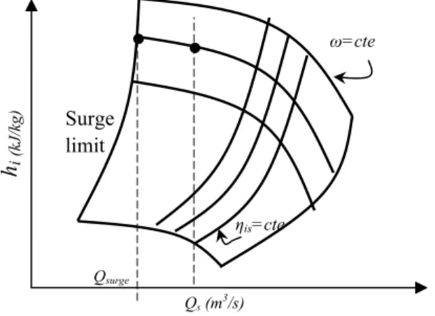
As shown on Figure 1, a centrifugal gas compressor is characterized by delivered flow rate and pressure ratio, the ratio between suction side pressure of the compressor and its discharge pressure. The compression process in a centrifugal compressor can be well formulated using isentropic process for calculating horsepower for a compressor station. The pressure ratio of a centrifugal

compressor is usually linked with a specific term named "head" carried over from pump design nomenclature and expressed in kJ/kg for compressors. The "head" developed by the compressor is defined as the amount of energy supplied to the gas per unit mass of gas.

Figure 1. A typical centrifugal compressor map The equation for power calculation can be expressed as follows:

is i ach m Pw    (15)

where m (kg/s) is the mass flow rate of compressed gas, h_ac i (kJ/kg) the compressor isentropic head, ηis the compressor isentropic efficiency.

For adiabatic compressor the adiabatic efficiency is defined by:

w ideal w is P P_,   (16)

As shown in the following equation, head is an index of the pressure ratio across the compressor. In this equation, pd is the discharge pressure of the compressor and ps, the suction pressure. The compressibility factor and the temperature here are considered at suction side of the compressor, where M is the average molecular mass of the gas (Smith and Van Ness, 1998).

Qs (m3/s) hi (kJ/kg) ω=cte ηis=cte Qsurge Surge limit

        ( )  1 1 -1     s d s s i p p M RT Z h (17)

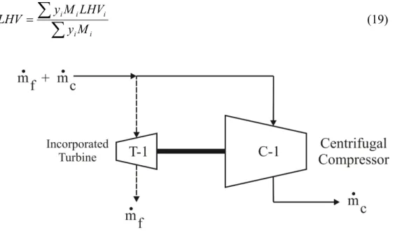
Centrifugal compressors in the station are assumed to be driven by turbines whose supply energy is provided from a line of the gas derived from the pipeline passed through the station in order to be compressed as shown in Figure 2. The flow rate of the consumed gas as fuel for the compression process in each compressor is obtained by dividing required power for compression, Pw, by the mechanical efficiency, ηm, driver efficiency, ηd and LHV (low heating value):

LHV n n n h m m d m is i ac f   3 10  (18)

According to Abbaspour et al. (2005), we have chosen a value of _m (respectively_d) equal to 0.90 (respectively 0.35). LHV represents the quantity of energy released by mass unity of the gas during complete combustion. It is considered at 298°K and 1 bar in (kJ/kg) and is calculated from the mass lower heating values, LHVi of the molecules composing the gas (Mi is the molecular mass of specie i):





Figure 2. Representation of the centrifugal compressor and its incorporated turbine

The adiabatic efficiency _is is defined by Eq. (21). Applying standard polynomial curve-fitting procedures for each compressor, the normalized head hi/ω2 can thus be obtained under the form of the following equation (Abbaspour et al., 2005). 2 3 2 1 2 _ (_ ) i s s Q b Q b b h    (20)

where Qs is the volumetric flow rate (m3/s).

In the same way, contours of constant isentropic efficiency could be fitted in the polynomial form of second degree shown in Eq. (21):

2 6 5 4 _ (_ )  s s is Q b Q b b    (21)

The rotational speed  (defined from Eq. 17 and 20) of all compressors is comprised between lower and upper bound as represented below. To prevent from surge phenomenon, by considering a surge margin, λsurge, the following constraint is introduced (Odom, 1990): u l      (22) s surge s surge _Q Q Q -  (23)

There is a surge flow rate, Qsurge, corresponding to each compressor rotational speed (Pugnet, 1999):

2 / 1 2 1 2 2 7 ( ) ) ( ) ) 1 (( M p RT Z M p RT Z h Mp RT Z b Q s s s s s s surge s s s surge         (24)

In this equation, hsurge is the surge head at a specified compressor speed and can be calculated using following equation:

2 3 2 1 2 _ ( _ )  surge surge surge Q b Q b b h    (25)

Considering a fixed value for a given surge efficiency, the surge efficiency will be introduced as a parameter during the optimization procedure. To avoid chocking occurrence at inlet, the following inequality should be considered.

) 1 ( 2 1 1 2            c A Q_{s s} (26)

As is the cross sectional area and c is the gas sonic velocity at the compressor inlet. Another inequality is introduced corresponding to the protection of a compressor against chocking phenomenon in impeller passages as shown in Inequality (27). In this expression, the impeller radius, r in (m) and A, the flow rate area in (m2), are considered at the section of rotating passages as well as Q, Z, T, p. The index 1 indicates the impeller inlet state.

) 1 ( 2 1 2 1 2 1 1 1 / ) )( 1 ( 2                  cA r c pM ZRT Q (27)

To prevent from diffuser choking, another inequality similar to that of the compressor inlet is considered, but as shown below, in this relation the gas properties are in the conditions of the diffuser and index 2 is used for diffuser inlet. ) 1 ( 2 1 02 02 1 2             _f f f f f c A M p RT Z Q (28)

Representing network topology by using incidence matrices

The different links between the elementary sections of a network can be defined using incidence matrices. Each pipe, each compressor and each fuel stream are represented by an arc. Consider a network with Nn nodes, Np pipe arcs and Nc compressor arcs. Therefore, there will be Nc fuel streams since for each compressor unit there is a stream that carries fuel to it. Because in a compressor, compression process is carried out, a compressor unit can be named an active arc. In this way, a pipe segment, in where the pressure decreases, may be called a passive arc. Let us note that the fuel streams have been considered as inert arcs regarding pressure change through them. A flow direction is assigned preliminarily to each pipe that can or not coincide with the real flow direction of

the gas that running through the arc. Nv valves can be introduced into the network to break the pressure between some pairs of arcs in order to balance the network.

Let A be a matrix of dimension Nn(Np Nc NV), where each of its

elements, aij, is given the following attribution:

       otherwise 0 i node into goes j arc if 1 i node from out comes j arc if 1 ij a (29)

A is called the node-arc incidence matrix. Similarly, let B be another matrix of dimension N_p N_c whose elements, bij, are defined below and it is named the pipe-compressor incidence matrix:

       otherwise 0 j compressor of node suction to connected is i pipe if 1 j compressor of node discharge to connected is i pipe if 1 ij b (30)

The last matrix is the node-fuel incidence matrix which describes the existing fuel stream derivations from a node, and it is called the compressor-fuel matrix. The dimension of this matrix is N_n N_c and elements are defined below:

    otherwise 0 j node from derived be i stream fuel if 1 ij c (31)

This matrix indicates which fuel stream belongs to which compressor.

These three incidence matrices are used to write the material balances around each node i, the flow rate of the consumed gas as fuel for the compression process in each compressor, and the equation of movement. For example, the material balance around the node i is expressed as Eq. (32). In this equation Si represents the gas delivery or supply relative to this node. It is negative if the node is a delivery one and positive for a supply node where the gas is injected to the node. i s compressor j i j f j arcs j i j j S m b m a 





Optimization procedures

Previous works

Monobjective optimization

A great diversity of optimization methods was implemented to meet the industrial stakes and provide competitive results. But if they prove to be well fitted to the particular case they consider, the numerical performances cannot be constant whatever the treated problem is. Actually, the efficiency of a given method for a particular example is hardly predictable, and the only certainty we have is expressed by the No Free Lunch Theory (Wolpert and Macready, 1997): there is no method that outdoes all the other ones for any considered problem. Among the diversity of optimization techniques, two important classes have to be distinguished: deterministic methods and stochastic ones. Complete reviews are proposed in literature for the two classes (Hao et al., 1999; Grossmann, 2002, Biegler and Grossmann, 2004). A thorough analysis of both classes was previously studied by Ponsich (2005) with the support of batch plant design problems.

The deterministic methods assume the verification of mathematical properties of the objective function and constraints, such as continuity, differentiability and convexity. In practice, these assumptions (particularly convexity) do not always hold, and the convergence towards a global optimum is no longer guaranteed. This working mode enables only to ensure to get a local optimum, which is for all that a great advantage versus stochastic methods. Among the deterministic class, particularly for NLP and MINLP problems, the following procedures can be mentioned: the Outer Approximation algorithm (Duran and Grossmann, 1986), the Branch & Bound methods for scanning trees (Gupta and Ravindran, 1985; Ryoo and Sahinidis, 1995; Smith and Pantelides, 1999), the Generalized Benders Decomposition (Geoffrion, 1972), the Extended Cutting Plane method for problems with a moderate degree of nonlinearity (Westerlünd and Petterson, 1995), disjunctive programming for quasi-convex problems (Raman and Grossmann, 1995). Even though most of the above-mentioned methods are only academic tools, some computational codes are available: the SBB, BARON, DICOPT++ and LOGMIP solvers within the GAMS modelling environment (Brooke et al., 2004), MINLP_BB (Leyffer, 1999) and ECP (Westerlünd and Lundqvist, 2003). Concerning the global optimization of non convex problems, the interval analysis method (Kearfott, 2001, Csendes, 2004) is a promising tool, but restricted at the present time to small problems, due to very high computational times.

The second class, namely stochastic methods, is based on the evaluation of the objective function at different points of the search space. These points are chosen through a set of heuristics, combined with generations of random numbers. Thus, stochastic procedures cannot guarantee to obtain an optimum.

However by allowing occasional objective function increases (for minimization problems) they may go out of local optimum gaps. They are divided into neighbourhood techniques such as Simulated Annealing (Kirkpatrick et al., 1982), Tabu Search (Teh and Rangaiah, 2003), and evolutionary algorithms comprising genetic algorithms (Holland, 1975), evolutionary strategies (Beyer and Schwefel, 2002) and evolutionary programming (Yang et al., 2006). Even if stochastic methods do not require any mathematical property for the objective function and constraints, they are difficult to implement for problems involving a significant number of equality constraints.

Multiobjective optimization

In many real world cases, the problem often involves several competing measures of performance, or objectives (Collette and Siarry, 2002). Using the formulation of multiobjective constrained problems of Fonseca and Fleming, (1998), a general multiobjective problem is made up of a set of n criteria fk, k = 1, …, n to be minimized or maximized. Each fk may be nonlinear with respect to the decision variable vector x in an m-dimensional universe U.

 



 

 



f  ₁ ,_, _n (33)

This kind of problem has not a unique solution in general, but presents a set of non-dominated solutions, named Pareto-optimal set or Pareto-optimal front. The Pareto-domination concept lies on two basic rules:

In the universe U a given vector u = (u1, …, un) dominates another vector v = (v1, …, van), if and only if,









i    

 1,_, : 1,_, : (34)

For a concrete mathematical problem, Eq. 34 gives the following definition of the Pareto front: for a set of n criteria, a solution f(x), related to a decision variable vector x = (x1, …, xm), dominates another solution f(y), related to y = (y1,…, ym) when the following condition is checked (for a minimization problem),





 

 





 

 

i _i  _i   _i  _i

The last definition concerns the Pareto optimality: a solution xu  U is called Pareto-optimal if and only if there is no xv  U for which v = f(xv) = (v1, … , vn) dominates u = f(xu) = (u1, … , un). These Pareto-optimal non-dominated individuals represent the solutions of the multiobjective problem. In practice, the decision maker has to select a single solution by searching among the whole Pareto front, and it may be difficult to pick one “best” solution out of a large set of alternatives. Branke et al. (2004), and Taboada and Coit (2006) suggest picking the knees in the Pareto front, that is to say, solutions where a small improvement in one objective function would lead to a large deterioration in at least one other objective. Other MCDM methods (Miettinen, 1999) like Topsis (Olson, 2004), can be used.

As in the monobjective case, for solving a multiobjective optimization problem, two classes of numerical methods are available. In the deterministic approach, the MOOP (MultiObjective Optimization Problem) is solved by means of NLP or MINLP procedures by optimizing a unique objective resulting from the aggregation of the various conflicting objectives to be optimized (Sawaragi et al., 1985). Classical toolboxes like GAMS or MATLAB can be used. The Pareto front is obtained by scanning the search space corresponding to the possible values of weighting factors. Another approach, called -constraint method consists in optimizing a single objective function, the other objective being considered as parameterized constraints (Mavrotas, 2006, Bérubé et al., 2009). The major inconvenience of these methods is that they are highly dependent on the choice either of weighting factors or of the RHS of the constraints defined by the objectives.

An alternative way consists in implementing stochastic methods. All the algorithms cited above can be adapted to the multiobjective case, and as it can be observed in the list of references recently proposed by Coello Coello (2009). Since 1990, the number of published papers per year is very important (more than 3700). Starting from a quasi null value in 1990, this number continuously increases, reaching 100 in 1995, 200 in 2000, 400 in 2005 and 500 the last year. The analysis of the list shows that genetic algorithms (GA) are cited in almost 40% of cases, and far behind them they are simulated annealing and particle swarms, followed by tabu search and differential evolution algorithms, then come the ant colonies and artificial neural networks, followed by constraint propagation methods, honeybee colonies, artificial immune systems and Monte-Carlo procedures. The two most popular methods in the chemical engineering field are MOGA (MultiObjective Genetic Algorithm, see Konac et al., 2006), and MOSA (MultiObjective Simulated Annealing, see Shu et al., 2004, Smith et al., 2004, Bandyopadhyay et al., 2008). None of these two methods is perfect and selecting one depends on the requirements of the particular design situation considered. From the literature survey (Van Veldhuizen and Lamont, 2000, Branke et al.,

2004, Turinsky et al., 2005, Mansouri et al., 2007) it appears that MOGA is generally preferred to MOSA.

Choice of optimization methods

The compressor adjustment problem presented in the next section is a NLP one, first solved for minimizing the total fuel consumption in compressors at the compression stations, and then solved in the multiobjective case by considering besides the fuel consumption, the throughput (delivery gas mass flow) of the system. As mentioned above, in the monobjective case, the deterministic methods are the most efficient. A solver (CONOPT3) of the GAMS environment was chosen, since this optimization package is widely used, and even stands as a reference for the solution of problems coming from the Process Systems Engineering field. The MATLAB optimization toolbox (namely FMINCON) was also used for comparison purposes.

In the multiobjective case, two solution methods are implemented and compared. A genetic algorithm called NSGA-IIb belonging to the genetic algorithm library (MULTIGEN) recently developed in the research group by Gomez (2008) has been first retained. Compared with the well-known NSGA II of Deb et al (2002), new genetics operators are introduced for clones creation limiting. The classical crossover operator SBX has been modified to produce children different from parents. The objective is to prevent unnecessary calculations for clones of existing solutions: all solutions generated by the crossover and mutation procedures are statistically different (Gomez, 2008). The set of constraints is made up of mass and momentum balances on the one hand and of compressor equations on the other hand. The numerical solution of this set of equations must be done carefully, making sure that the equality system of equations captures all the relevant aspects of the associated network problem. This square set of nonlinear equations is parameterized by the optimization variables (rotational speeds of compressors), and so the MOOP is solved by means of a two-stage strategy. At the upper level the GA returns values of the rotational speeds, which are reported into the set of constraints, written under the format of MATLAB R2008a and solved by a Newton-Raphson procedure of the MATLAB toolbox. To efficiently solve this set of nonlinear equations, suitable variable bounds and initial values have to be applied at each node of the network. These values are taken from Tabkhi’s PhD Thesis (2007).

The second method implemented is the -constraint procedure. In this method one of the objective functions is minimized while all the other objective functions are upper bounded by introducing supplementary constraints. So the multiobjective problem is transformed into the following monobjective one:

U x x f_k  ) ( Min

with the additional constraints: (36)

, to 1 , ) (x i n i k f_i _i  

By parametrical variation in the RHS of the constrained objective functions the efficient solutions of the problem can be obtained. In order to properly apply the ε-constraint method, the range of the n-1 objective functions that are used as constraints, must be known. The calculation of the range of the objective functions over the efficient set is not a trivial task. While the best value is easily attainable as the optimum of the individual optimization, the worst value over the efficient set (Nadir value) is not. The most common approach is to calculate these ranges from the payoff table (the table with the results from the individual optimization of the n objective functions). From Ehrgott and Wiecek (2005), the optimal solution of problem (36) is guaranteed to be an efficient solution only if all the (n-1) objective function constraints are binding. To overcome this difficulty, Mavrotas (2006) proposes the transformation of the objective function constraints to equalities by explicitly incorporating the appropriate slack or surplus variables. In the same time, the sum of these slack or surplus variables is used as a second term (with lower priority) in the objective function forcing the program to produce only efficient solutions. A quite similar approach based on slack variables is presented by Ehrgott and Ruzika (2008).

Numerical example: compressor adjustment problem

Network characteristics

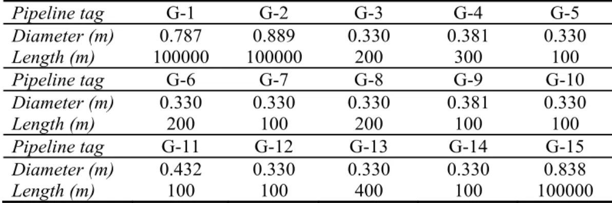
The example is inspired from the work of Abbaspour et al. (2005) (see Figure 3). The network consists of three long pipelines of 100 kilometres. There are two compressor stations that operate to compensate for pressure drop in the pipelines. Each compressor station includes three parallel centrifugal compressors. In each station, there are six short pipe segments of about a hundred meters linked to the entrances and outlets of the compressors. Although the length and the diameter of these pipes is lower than those of the three major pipelines, their role in the pressure change through the network may not be negligible and may even sometimes become bottleneck of the system. Therefore, these pipelines are also considered in the model. The technical features of the pipeline system corresponding to Figure 3, considered as fixed parameters for the optimization problem, are proposed in Table 1.

Figure 3. Schema of the considered pipeline network

Table 1.Technical features of the pipelines of the system shown in Figure 3

Pipeline tag G-1 G-2 G-3 G-4 G-5 Diameter (m) 0.787 0.889 0.330 0.381 0.330 Length (m) 100000 100000 200 300 100 Pipeline tag G-6 G-7 G-8 G-9 G-10 Diameter (m) 0.330 0.330 0.330 0.381 0.330 Length (m) 200 100 200 100 100 Pipeline tag G-11 G-12 G-13 G-14 G-15 Diameter (m) 0.432 0.330 0.330 0.330 0.838 Length (m) 100 100 400 100 100000 G1 G2 G3 G4 G9 G8 G7 G15 G5 G12 G6 G10 G13 G11 G14 1 2 3 4 5 6 7 14 15 8 9 10 11 12 13 16 0 17 C1 C2 C3 C4 C5 C6 Supply Delivery

compressors are assumed to be 0.90 and 0.35 respectively according to values proposed in the dedicated literature (Menon, 2005).

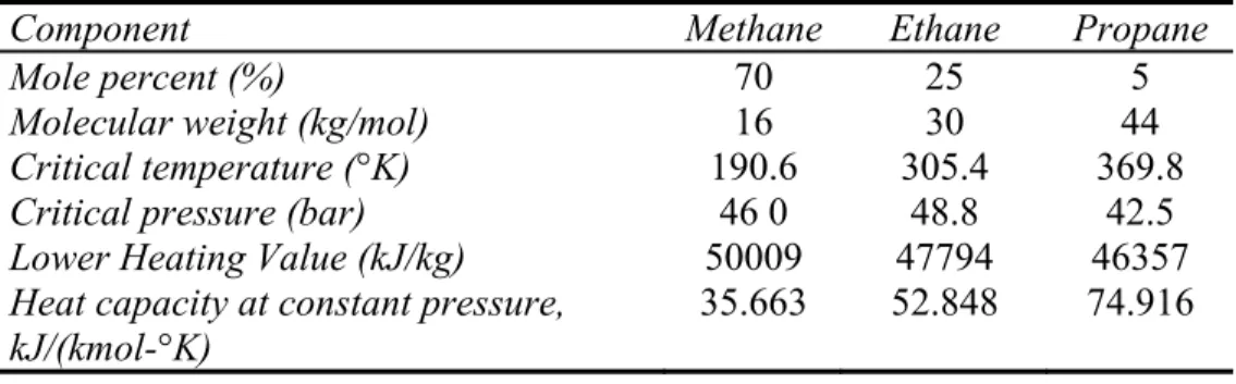
Table 2. Thermodynamic properties of the components of gas flowing in the pipelines

Component Methane Ethane Propane

Mole percent (%) 70 25 5

Molecular weight (kg/mol) 16 30 44

Critical temperature (°K) 190.6 305.4 369.8 Critical pressure (bar) 46 0 48.8 42.5 Lower Heating Value (kJ/kg) 50009 47794 46357 Heat capacity at constant pressure,

kJ/(kmol-°K)

35.663 52.848 74.916

The network includes 18 nodes, 15 pipes arcs and 6 compressor arcs. As for each compressor unit, there is a stream that carries fuel to it; there are 6 fuel streams which have not been shown in Figure 3 to avoid complexity. For each compressor, this stream originates from suction node. A flow direction is assigned to each pipe so the gas flows from 0 to 17. For example, the node-arc incidence matrix A (see Table 3) is a matrix of dimension 18 × (15+6) (the network does not involve any valve). The material balance around the nodes can be stated in a very concise way by using this matrix.

Roughness of inner surface of the pipes is considered to be equal to 46×10-6 (traditional value reported for stainless steel). The temperature is assumed to be isothermal and equal to 330°K all over the system. The adiabatic efficiency _is is defined by Eq. (21), and mechanical efficiency and driver efficiency for the The pressure is considered to be equal to 60 bar with a margin of ±2% at the entrance point of the network, node 0, as well as the delivery pressure, at node 17 (in other words the lower bound is 58.8 bar and the upper one is 61.2 bar). The gas flows from node 0 towards node 17, and there is no input or output in the other nodes. The typical composition of NG considered in the numerical runs is presented in Table 2 with also the thermodynamic properties of gas components.

Table 3. Node-arc incidence matrix corresponding to Figure 3 (+ represents +1, - represents -1, blank represents 0)

G 1 G2 G3 G4 G5 6 G G7 G8 G9 G 10 G 11 G 12 G 13 G 14 G 15 C1 2 C C3 C4 C5 C6 Node + 0 _ + + + 1 _ + 2 _ + 3 _ + 4 + _ 5 + - 6 + _ 7 _ + 8 _ + 9 _ + 10 + _ 11 + _ 12 + _ 13 _ _ _ + 14 + + + _ 15 + _ _ _ 16 _ 17

Monobjective case: total fuel consumption optimization

NLP formulation

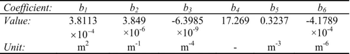
The continuous variables of this problem are: 18 pressure variables governing the nodes and 21 flow rate variables (including fuel streams) corresponding to pipes and compressors. The rotational speeds of the compressors have not been explicitly considered as variables, since the flow rates of the fuel streams have already been considered as variables for each compressor. As shown in Eq. (18) to (25), the rotational speeds are directly dependent on the fuel stream flow rates. The coefficients bi of Eq. (20) and (21) are reported in Table 4.

Table 4. Coefficients of the isentropic head equation and coefficients of the isentropic efficiency equation of the compressors

Coefficient: b1 b2 b3 b4 b5 b6 Value: 3.8113 4 10  3.849 ×10-6 -6.3985×10-9 17.269 0.3237 -4.1789 ×10-4 Unit: m2 m-1 m-4 - m-3 m-6

The equality constraints consist of 18 mass balances around nodes, 15 equations of motion for the pipe arcs, 6 isentropic head equations for compressors as shown in Eq. (17), 6 relationships between rotational speed, suction volumetric flow rate and head of each compressor (Eq. 20), 6 equations to calculate isentropic efficiency according to Eq. (21), 6 equations to determine fuel consumption at each compressor unit. The set of inequality constraints is constituted by a lower bound for delivery flow rate (flow rate in arc G2) equal to 150 kg/s, an upper bound as well as a lower bound for the pressures of the nodes (MAOP as an upper bound and atmosphere pressure as a lower bound, the following values were chosen for computing the MAOP: fF = 0.72, fE = 1, fT = 1), sonic velocity and erosional velocity in the role of upper bounds of the velocities through pipes, lower and upper bounds on the rotation speed of all compressors (166.7 and 250 rps respectively), a lower bound on compressor throughput in order to avoid pumping phenomenon, an upper bound on compressor throughput to prevent from chocking phenomenon. In total, there are 57 equality constraints and 76 inequality constraints.

The total sum of the fuel consumption in compressors is the objective function, as expressed in Eq. (37). For each compressor, fuel consumption flow rate,

i f

m is obtained by using Eq. (18).



As indicated above, in this monobjective case, the solver CONOPT3 of the GAMS package has been retained for solving the problem. The initialization of the variables is performed directly through the software CONOPT3 under the condition that the problem is well-scaled and that bounds are assigned adequately. For bounded variables, CONOPT3 takes the initial values in the middle of the bounds. Several other initial points were randomly selected (inside the bounds, for bounded variables), the same solution was obtained. Strictly considering the nonconvexity feature, the example is not so strongly nonconvex.

The options used for implementing CONOPT3 are following: optimality tolerance = 10-8, maximum feasibility tolerance = 10-5, number of stalled iterations = 100. The resolution takes about 0.5s CPU on a PC (processor Intel Core 2 Duo, 2.99 GHz, RAM 1.96 Go). With same tolerances MATLAB gives identical results, but the CPU time is higher (a few seconds). Table 5 presents the results relative to pressure values at each node. Observe that at node 0 (i.e., supply node), the algorithm has taken the maximum possible pressure (61.2 bar) whereas

the minimum possible value (58.8 bar) was obtained at node 17 (i.e., delivery node).

Table 5. Pressure of NG at all of the nodes of the pipeline network

Node Pressure (bar)

Node Pressure (bar)

0

61.2

9

58.3

1

47.4

10

58.4

2

47.0

11

65.2

3

47.1

12

65.5

4

47.2

13

65.2

5

67.0

14

66.8

6

66.9

15

58.4

7

67.0

16

65.0

8

58.3

17

58.8

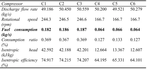
The value of objective function that is the total fuel consumption in the compressor stations is equal to 0.749 kg/s (sum of individual compressor consumptions, see Table 6, bold line) leads to a significant reduction of 13% from the initial solution (0.863 kg/s for initial values between their bounds). Other results are listed in Table 6. The optimum percentage of the input gas that is consumed in the stations can thus be calculated and is found equal to 0.499 %. For each compressor, consumption ratio is defined as the fuel consumption divided by the input mass flow rate. Let us mention in this example that the compressors involved in the second station work at their minimum rotational speeds, whereas the compressors of the first station work close to their maximum speeds. Finally, the transmitted power of the pipeline, that is the product of the pipeline delivery throughput (150 kg/s) and the lower heating value (LHV) of the NG (48830 kJ/kg) is found to be equal to 7324 MW at this optimal point.

Table 6. Optimal values of discharge flow rates, rotational speeds, fuel consumptions, isentropic head and isentropic efficiency for the compressor units

of the network

Compressor C1 C2 C3 C4 C5 C6

Discharge flow rate (kg/s) 49.186 50.450 50.559 50.200 49.521 50.279 Rotational speed (rpm) 244.3 246.5 246.6 166.7 166.7 166.7 Fuel consumption (kg/s) 0.182 0.186 0.187 0.064 0.066 0.064 Consumption ratio (%) 0.369 0.367 0.369 0.127 0.133 0.127 Isentropic head (kJ/kg) 42.592 42.188 42.201 12.664 13.367 12.607 Isentropic efficiency (%) 74.917 74.215 74.207 64.195 65.331 64.101 The Lagrange multipliers obtained at the solver convergence can be used to carry out a sensitivity analysis. All these parameters are null or quasi-null except for the supply pressure at node 0 (value=-0.047) and the delivery pressure at node 17 (value 0.017). This means for example that if the supply pressure is increased of one bar, the total fuel consumption will be decreased of 0.047 kg/s. In the same way, if the delivery pressure is decreased of one bar, the total fuel consumption will be decreased of 0.017 kg/s.

Carbon dioxide emissions

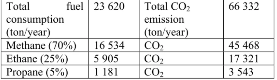
The total fuel consumption in the compressor stations is found equal to 0.749 kg/s, that is to say 23 640 ton/year. The combustion reaction of one molecule of methane (molar mass = 16 g) produces one molecule of CO2 (molar mass = 44 g). One molecule of ethane (molar mass = 30 g) gives two molecules of CO2, and for one molecule of propane (molar mass = 44 g), three molecules of CO2 are obtained.

The results are summarized in Table 7. The carbon dioxide emissions are 66 332 ton/year. Let us recall that the NG delivery is 150 kg/s that is to say 4 730 400 ton/year. The carbon dioxide emissions represent only 1.4% of the delivery gas, which is very acceptable.

Table 7. CO2 emissions Total fuel consumption (ton/year) 23 620 Total CO2 emission (ton/year) 66 332 Methane (70%) 16 534 CO2 45 468 Ethane (25%) 5 905 CO2 17 321 Propane (5%) 1 181 CO2 3 543

Multiobjective case: total fuel consumption minimization and NG

delivery maximization

Problem formulation

In the previous section the fuel consumption in the compressor stations was minimized for a given gas mass flow delivery. However for a natural gas delivery Company, the demand may vary according to climatic conditions or industrial requirements. So the problem which arises is to determine, for a given supply at the network entrance nodes, the minimal and maximal network capacities in terms of NG mass flow delivery and fuel consumption in compressor stations. This problem can be formulated as a biobjective optimization problem.

In fact, it’s not about a problem a decision making strictly speaking, as far as the practical problem formulates as follows. For a NG delivery Company, the total mass flow delivery is imposed on a given period, and the problem is to operate the compressor stations so as to minimize the fuel consumption in the stations. When performing the biobjective optimization, the Pareto front (see Figure 4) provides an easy way for:

1 – identifying the minimum and maximum network capacities in terms of mass flow delivery and fuel consumption;

2 – for a given mass flow delivery between the above bounds, the minimal fuel consumption and thus the minimal carbon dioxide emission can be deduced.

Concerning the optimization variables and constraints, the problem is identical to the previous one, but here the NG mass flow delivery is not fixed at 150 kg/s. The goal is to simultaneously minimize the total fuel consumption (this objective is noted f1) in the compressor stations, while maximizing the NG delivery mass flow (objective noted f2).

Problem solution

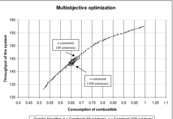
As mentioned above, the solver NSGA-IIb of the MULTIGEN library, coupled with a Newton-Raphson procedure was implemented for solving the multiobjective problem. To simplify the scanning of the search space, it was assumed that the rotational speeds can only take integer values. The options used for implementing NSGA-IIb are: population size = 100, maximum number of generations = 300. The GA was run 10 times with different initial values for the rotational speeds (randomly generated); the Pareto front (symbols crosses) reported on Figure 4 has been obtained five times. The resolution of one GA takes an average time of 9 hours CPU on the same PC as above.

Figure 4. Pareto front

Relevant information lies in the two extreme points of the front, insofar as they represent the minimum and maximum capacities of the network in terms of NG delivery and fuel consumption. These solutions were verified by performing monobjective optimizations of the fuel consumption for a NG mass flow delivery of 133 kg/s and then of 157 kg/s; the same solutions for the fuel consumption

Multiobjective optimization 130 135 140 145 150 155 160 0.4 0.45 0.5 0.55 0.6 0.65 0.7 0.75 0.8 0.85 0.9 0.95 1 1.05 1.1 Consumption of combustible Thr ou ghput of t h e syst em

Genetic Algorithm ε-Constraint (40 solutions) ε-Constraint (100 solutions)

ε-constraint (40 solutions)

ε-constraint (100 solutions)

were found again. Conversely, the NG mass flow delivery was computed with compressor rotational speeds given at the two extreme points, the mass flow delivery of 133 kg/s and of 157 kg/s were obtained again.

It can be observed on the Pareto front, that for NG mass flow delivery of 150 kg/s, the same value (0.749 kg/s) of the total fuel consumption as in the monobjective case is found again. The values of pressures, discharge flow rates, rotational speeds, fuel consumptions, isentropic head and isentropic efficiency for the compressors are the same as the ones listed in Tables 5 and 6. The carbon dioxide emissions are given in Table 7.

A supplementary verification was carried out by implementing the -constraint method. The obtained front is given by symbols circles for 40 generated solutions and triangles for 100 generated solutions on Figure 4. The two fronts obtained from genetic algorithm and -constraint are superimposed but the front of -constraint is much more restricted than the one of genetic algorithm. If the problem was a MCDM one, the -constraint would be a more efficient tool than the genetic algorithm due to its restricted front.

From these checks, we can assume that the Pareto front given by the genetic algorithm is correct and brings more information because more extended than the one of -constraint.

Carbon dioxide emissions

For the pair (f1 = 0.749 kg/s, f2 = 150 kg/s), the results are reported in Table 7. Two new studies for the extreme solutions (case 1: f1 = 0.540 kg/s, f2 = 133 kg/s) and (case 2: f1 = 0.980 kg/s, f2 = 157 kg/s) are carried out, the results are indicated in Tables 8 and 9.

Case 1

The carbon dioxide emissions are 47 823 ton/year (see Table 8). The NG delivery is 133 kg/s that is to say 4 194 288 ton/year. The carbon dioxide emissions represent 1.1% of the delivery gas.

Table 8. CO2 emissions (case 1) Total fuel consumption (ton/year) 17 029 Total CO2 emission (ton/year) 47 823 Methane (70%) 11 920 CO2 32 780 Ethane (25%) 4 257 CO2 12 487 Propane (5%) 852 CO2 2 556

Case 2

The carbon dioxide emissions are 86 794 ton/year (see Table 9). The NG delivery is 157 kg/s that is to say 4 951 152 ton/year. The carbon dioxide emissions represent 1.8% of the delivery gas.

Table 9. CO2 emissions (case 2) Total fuel consumption (ton/year) 30 905 Total CO2 emission (ton/year) 86 794 Methane (70%) 21 635 CO2 59 496 Ethane (25%) 7 726 CO2 22 663 Propane (5%) 1 545 CO2 4 635 Discussion

Along the Pareto front, the carbon dioxide emissions vary from 1.1% to 1.8% of the NG mass flow delivery. These values are very lower than those usually admitted; indeed as mentioned in the Introduction section it is estimated (Suming et al., 2000) that the compressor stations typically consume about 3 to 5% of the transported gas. So the optimization of compression operations yields significant savings for the fuel consumed in the stations.

Conclusion

Efficient operation of compressor stations is of major importance for enhancing the performances of pipeline networks. In this paper, a pipeline network system including two compressor stations is optimized by implementing two strategies. In the monobjective case a deterministic optimization procedure is used. In the multiobjective case a genetic algorithm and a -constraint method are implemented and compared. A didactic example coming from the literature illustrates the approach.

In the monobjective study, the objective function is the total fuel consumption in the compressor stations to be minimized for a fixed gas delivery mass flow, since reduction of the energy used in pipeline operations will have a significant economical impact. Typical results are analyzed and the characteristic values of some key parameters like isentropic head and isentropic efficiency are computed. The numerical results show that numerical optimization is an effective tool for optimizing compressor rotational speeds, and can yield significant reductions in fuel consumption. The carbon dioxide emissions evaluated at the

optimal solution represent only 1.4% of the delivery gas, which is very acceptable.

For the multiobjective study, the goal consists in simultaneously minimizing the total fuel consumption while maximizing the gas mass flow delivery. The problem is solved by means of a genetic algorithm and -constraint procedure. The two methods give superimposed Pareto fronts, but the one from genetic algorithm is much larger than the one from -constraint.

Along the Pareto front provided by the genetic algorithm, the carbon dioxide emissions vary from 1.1% to 1.8% of the NG mass flow delivery. It is estimated that the compressor stations typically consume about 3 to 5% of the transported gas. So the optimization of compression operations yields big savings for the fuel consumed in the stations, and thus has a real environmental impact. Contrary to classical decision making problems, where the best points have to be found on the Pareto front by searching “knees” on the front or by using MCDM method like Topsis, the Pareto front supplies two significant information. First, bounds on the network capacity in terms of mass flow delivery and CO2 emissions can directly be obtained from the curve. Second, for an imposed mass flow delivery that corresponds to practical case for a NG delivery Company, the minimal fuel consumption directly linked to CO2 emissions can be obtained by tuning compressor stations (particularly rotational speeds of compressors) at values provided by the optimizer.

References

Abbaspour M., Chapman K.S. and P. Krishnaswami, “Nonisothermal compressor station optimization”, Journal of energy resources technology, 2005, 127, 131-141.

André J., Bonnans F. and L. Cornibert, “Planning reinforcement on gas transportation networks with optimization methods”, Process Operation Research Models and Methods in the Energy Sector Conference, ORMMES, Coimbra, Portugal, 2006.

Bandyopadhyay S., Saha S., Maulik U. and K Deb, “A simulated annealing–based multiobjective optimization algorithm: AMOSA”, IEEE Trans Evolutionary Computation 12, 2008, 269-283.

Bérubé J.F, Gendreau M. and J.Y. Potvin, “An exact e-constraint method for bi-objective combinatorial optimization problems”, European Journal of Operational Research, 2009, 39-50.

Beyer H.G. and H.P. Schwefel, “Evolution strategies, a comprehensive introduction”, Natural Computing, 2002, 1, 3-52.

Biegler L.T. and I.E. Grossmann, “Retrospective on optimization”, Computers and Chemical Engineering 2004, 28, 1169-1188.

Boyd E.A., Scott L.R. and S.S. Wu, “Evaluating the quality of pipeline optimization algorithms”, 29th annual meeting of Pipeline Simulation Interest Group, Tucson, 1997, 5-17 October.

Branke J., Deb K., Dierolf H. and M. Osswald, “Finding knees in multiobjective optimization, Parallel problems solving from nature”, in LNCS, Springer, 2004, 3242, 722-731.

Brooke A., Kendrick D., Meeraus A. and R. Raman, “GAMS: a user’s guide”, GAMS Development Corporation, Washington, 2004.

Chauvelier-Alario M., Mathieu B., and C. Toussaint”, Decision making software for Gaz de France distribution network operators”, Carpathe, 23rd World Gas Conference, Amsterdam, Netherlands, 2006.

Cobos-Zaleta D. and R.Z. Rios-Mercado, “A MINLP model for minimizing fuel consumption on natural gas pipeline networks”, XI Latin-Ibero-American conference on operations research, 2002, 27-31 October, Concepción Chile.

Coello Coello C.A., http://www.lania.mx./~coello/EMOO/EMOObib.html (2009). Collette Y. and P. Siarry, “Optimisation multiobjectif”, Eyrolles, 2002.

Costa A.L.H., de Medeiros J.L. and F.L.P.Pessoa, “Steady-state modelling and simulation of pipeline networks for compressible fluids”, Brazilian Journal of Chemical Engineering, 1998, 15, 344-357.

Csendes T., “Generalized subinterval violation criteria for interval global optimization”, Numerical Algorithms, 2004, 37, 93-100.

Deb K., Pratap A., Agarwal S. and T. Meyarivan, “A Fast and Elitist Multiobjective Genetic Algorithm: NSGA-II”, IEEE Transactions on Evolutionary Computation, 2002, 182-197.

Duran M.A. and I.E. Grossmann, “An outer-approximation algorithm for a class of mixed-integer nonlinear programs”, Mathematical Programming, 1986, 36, 307-339.

Ehrgott M. and M. Wiecek, “Multiobjective Programming, Multiple Criteria Decision Analysis. State of the Art Surveys”, J. Figueira, S. Greco, M. Ehrgott Eds, Springer, 2005, 667-722.

Ehrgott M. and S. Ruzika, “Improved -constraint method for multiobjective programming”, JOTA, 2008, 138, 375-396.

Fonseca C.M. and P.J. Fleming, “Multiobjective Optimization and Multiple Constraint Handling with Evolutionary Algorithm-Part I: A Unified Formulation”, IEEE Transactions on Systems, Man and Cybernetics – Part A: Systems and Humans, 1, 1998, 26-37.

Geoffrion A.M., “Generalized benders decomposition”, Journal of Optimization Theory and Applications, 1972, 10, 237-260.

Gomez A., « Optimisation technico-économique multi-objectif de systèmes de conversion d’énergie : Cogénération électricité-hydrogène à partir d’un réacteur nucléaire de IVème génération », Thèse de Doctorat de l’Université de Toulouse (Institut National Polytechnique), Toulouse, France, 2008.

Grossmann I.E., “Review of nonlinear mixed-integer and disjunctive programming techniques”, Optimization and Engineering, 2002, 3, 227-252.

Gupta O.K. and V. Ravindran, “Branch and bound experiments in convex nonlinear integer programming”, Management Science, 1985, 31, 1533-1546.

Hao J., Galinier P. and M. Habib, “Métaheuristiques pour l’optimisation combinatoire et l’affectation sous contrainte“, Revue d’intelligence Artificielle, 1999, 13, 283-324.

Holland J.H., “Adaptation in natural and artificial systems”, MI University of Michigan Press, 1975.

Kearfoot R.B., “Interval analysis: interval Newton method”, Encyclopedia of Optimization, 2001, 3, 76-78.

Kirkpatrick S., Gelatt J.C.D. and M.P. Vecchi, “Optimization by simulated annealing”, IBM Research Report, RC9355, 1982.

Konac A., Coit D.W. and A.E. Smith, “Multi-objective optimization using genetic algorithms: A tutorial”, Reliability Engineering and System Safety,91, 2006, 992-1007.

Lewandowski A, “Object-oriented modelling of the natural gas pipeline network”, 26th annual meeting of Pipeline Simulation Interest Group, San Diego, 1994, 13-14 October.

Leyffer S. “User manual for MINLP_BB”, University of Dundee, Numerical Analysis Report NA/XXX, 1999.

Mansouri S.A., Hendizadeh S.H. and N. Salmassi, “Bicriteria two-machine flowshop scheduling using metaheuristics”, GECCO’07, London, UK, CD-ROM, ISBN 978-59593-697, 2007.

Martinez-Romero N., Osorio-Peralta O. and I. Santan-Vite, “Natural gas network optimization and sensibility analysis”, Proceedings of the SPE International Petroleum Conference and Exhibition of Mexico, 2002, 357-370.

Mavrotas G., “Generation of efficient solutions in multiobjective mathematical programming problems using GAMS”, Tech. Rep., School of Chemical Engineering, National Tevhnical University of Athens, 2006.

Menon E.S., “Gas pipeline hydraulics“, Boca Raton, CRC Press, Taylor & Francis Group, 2005.

Miettinen K.M., “Nonlinear Multiobjective Optimization”, Kluwer Academic Publishers, 1999.

Mohitpour M., Thompson W. and B. Asante, “The importance of dynamic simulation on the design and optimization of pipeline transmission systems”, Proceedings of ASME International Pipeline Conference, 1996, 2, 1183-1188.

Mohring J., Hoffmann J., Halfmann T., Zemitis A., Basso G. and P. Lagoni, “Automated model reduction of complex gas pipeline networks”, 36th annual meeting of pipeline simulation interest group, Palm Springs, California, 2004.

Mora T. and M. Ulieru, “ Minimization of energy use in pipeline operations - an application to natural gas transmission systems”, Industrial Electronics Society, IECON, 31st annual conference of IEEE, 2005, ISBN 0-7803-9252-3.

Odom F.M., “Tutorials on modelling of gas turbine driven centrifugal compressors”, 22nd annual meeting of pipeline simulation interest group, Baltimore, Maryland, 1990.

Olson D.L., “Comparison of weights in TOPSIS model”, Mathematical and Computer Modelling, 2004, 40, 721-727.

Osiadacz A.J., “Dynamic optimization of high Pressure gas Networks using hierarchical systems theory”, 26th _{annual meeting of Pipeline Simulation} Interest Group, San Diego, 1994, 13-14 October.

Ponsich A. “Stratégies d’optimisation mixte en Génie des Procédés - Application à la conception d’ateliers discontinus“, PhD Thesis, Institut National Polytechnique de Toulouse, France, 2005.

Pugnet J.M., “Pompage des compresseurs“, Techniques de l'ingénieur, Génie mécanique, 1999, BL2 :BM4182.1-BM4182.18.

Raman R. and I.E. Grossmann, “Modelling and computational techniques for logic based integer programming”, Computers and Chemical Engineering, 1995, 18, 563-578.

Rios-Mercado R.Z., Wu S., Scott L.R. and E.A. Boyd, “A Reduction technique for natural gas transmission network optimization problems”, Annals of Operations Research, 2001, 117, 217-234.

Romeo E., Royo C. and A. Monzon, “Improved explicit equations for estimation of the friction factor in rough and smooth pipes, Chemical engineering journal, 2002, 86, 369-374.

Ryoo H.S. and N.V. Sahinidis, “Global optimization of nonconvex NLPs and MINLPs with applications in process design”, Computers and Chemical Engineering, 1995, 19, 551-566.