HAL Id: hal-01087279
https://hal.archives-ouvertes.fr/hal-01087279
Submitted on 5 Sep 2020
HAL is a multi-disciplinary open access
archive for the deposit and dissemination of
sci-entific research documents, whether they are
pub-lished or not. The documents may come from
teaching and research institutions in France or
abroad, or from public or private research centers.
L’archive ouverte pluridisciplinaire HAL, est
destinée au dépôt et à la diffusion de documents
scientifiques de niveau recherche, publiés ou non,
émanant des établissements d’enseignement et de
recherche français ou étrangers, des laboratoires
publics ou privés.
emissions inferred from SCIAMACHY, TANSO-FTS,
IASI and surface measurements
C. Cressot, F. Chevallier, P. Bousquet, C. Crevoisier, E.J. Dlugokencky, A.
Fortems-Cheiney, C. Frankenberg, R. Parker, I. Pison, R.A. Scheepmaker, et
al.
To cite this version:
C. Cressot, F. Chevallier, P. Bousquet, C. Crevoisier, E.J. Dlugokencky, et al.. On the consistency
between global and regional methane emissions inferred from SCIAMACHY, TANSO-FTS, IASI and
surface measurements. Atmospheric Chemistry and Physics, European Geosciences Union, 2014, 14
(2), pp.577-592. �10.5194/acp-14-577-2014�. �hal-01087279�
www.atmos-chem-phys.net/14/577/2014/ doi:10.5194/acp-14-577-2014
© Author(s) 2014. CC Attribution 3.0 License.
Atmospheric
Chemistry
and Physics
On the consistency between global and regional methane emissions
inferred from SCIAMACHY, TANSO-FTS, IASI and surface
measurements
C. Cressot1, F. Chevallier1, P. Bousquet1, C. Crevoisier2, E. J. Dlugokencky3, A. Fortems-Cheiney1, C. Frankenberg4, R. Parker5, I. Pison1, R. A. Scheepmaker6, S. A. Montzka3, P. B. Krummel7, L. P. Steele7, and R. L. Langenfelds7
1Laboratoire des Sciences du Climat et de l’Environnement, UMR8212, 91191 Gif-sur-Yvette, France 2Laboratoire de Météorologie Dynamique/CNRS/IPSL, Ecole Polytechnique, Palaiseau, France 3Climate Monitoring and Diagnostics Laboratory, NOAA, Boulder, Colorado, USA
4Jet Propulsion Laboratory, California Institute of Technology, Pasadena, California, USA 5Earth Observation Science, Space Research Centre, University of Leicester, Leicester, UK 6SRON Netherlands Institute for Space Research, Utrecht, the Netherlands
7Centre for Australian Weather and Climate Research, CSIRO Marine and Atmospheric Research, Aspendale, Victoria,
Australia
Correspondence to: C. Cressot (cindy.cressot@lsce.ipsl.fr)
Received: 22 February 2013 – Published in Atmos. Chem. Phys. Discuss.: 25 March 2013 Revised: 26 November 2013 – Accepted: 28 November 2013 – Published: 20 January 2014
Abstract. Satellite retrievals of methane weighted atmo-spheric columns are assimilated within a Bayesian inversion system to infer the global and regional methane emissions and sinks for the period August 2009 to July 2010. Inversions are independently computed from three different space-borne observing systems and one surface observing system under several hypotheses for prior-flux and observation errors. Pos-terior methane emissions are compared and evaluated against surface mole fraction observations via a chemistry-transport model. Apart from SCIAMACHY (SCanning Imaging Ab-sorption spectroMeter for Atmospheric CartograpHY), the simulations agree fairly well with the surface mole frac-tions. The most consistent configurations of this study us-ing TANSO-FTS (Thermal And Near infrared Sensor for carbon Observation – Fourier Transform Spectrometer), IASI (Infrared Atmospheric Sounding Interferometer) or sur-face measurements induce posterior methane global emis-sions of, respectively, 565 ± 21 Tg yr−1, 549 ± 36 Tg yr−1
and 538 ± 15 Tg yr−1over the one-year period August 2009–
July 2010. This consistency between the satellite retrievals (apart from SCIAMACHY) and independent surface mea-surements is promising for future improvement of CH4
emis-sion estimates by atmospheric inveremis-sions.
1 Introduction
Methane (CH4) is the second most important anthropogenic
greenhouse gas in terms of radiative forcing after carbon dioxide (Forster, 2007). CH4sources are of biogenic origin
(wetlands, rice cultivation, ruminant animals, termites, land-fills and waste), of pyrogenic origin (biomass burning) and of thermogenic origin (production, transport and distribution of fossil fuels, natural geological leakages). The emissions are about 2/3 anthropogenic and 1/3 natural, with large un-certainties for each individual source (20–100 %) (Kirschke et al., 2013). Its loss in the atmosphere, mainly controlled by its chemical reaction with hydroxyl free radical (OH), gives the CH4molecule a lifetime of about 9 yr. Methane
concen-trations have reached unprecedented values since the begin-ning of the industrial era (+150 %) and the explanation for their recent variability is still debated (Bousquet et al., 2011; Rigby et al., 2008). Methane sources and sinks are classically estimated either using bottom-up approaches (process-based modelling and inventories) or top-down approaches (atmo-spheric inversions). Atmo(atmo-spheric inversions, mostly based so far on surface CH4 observations (Houweling et al., 1999;
Bousquet et al., 2006; Bergamaschi et al., 2009, 2010; Pi-son et al., 2009), have shown to improve bottom-up methane
emission estimates from global to regional scales. One diffi-culty with atmospheric inversions is the determination of er-ror statistics attached to atmospheric observations and prior knowledge of emissions and sinks. More or less empirical methods have been set up by various authors to fill the as-sociated covariances matrices (Pison et al., 2009; Bergam-aschi et al., 2010; Chen and Prinn, 2006). These approaches generally rely on proxy methods and expert judgement. Since 2003, retrievals of methane mixing ratios from space are available from the SCanning Imaging Absorption spec-troMeter for Atmospheric CartograpHY (SCIAMACHY) on board the ENVIronmental SATellite (ENVISAT), largely increasing the number of available constraints for atmo-spheric inversions, but with a lower individual precision of measurements (∼ 2 %) as compared to surface observations (∼ 0.2 %). First inversions using SCIAMACHY retrievals have been produced, with the need for specific and empiri-cal treatment to account for retrieval biases (Meirink et al., 2008).
We study four different observing systems that measure or retrieve CH4 mole fractions (nmol mol−1, abbreviated
ppb): SCIAMACHY, the Thermal And Near infrared Sen-sor for carbon Observation – Fourier Transform Spectrome-ter (TANSO-FTS) on board the Greenhouse Gas Observing SATellite (GOSAT), the Infrared Atmospheric Sounding In-terferometer (IASI) on board the Meteorological Operational Polar satellite (MetOp) and surface air sample sites from various networks (the National Oceanic and Atmospheric Administration (NOAA), the Italian National Agency for New Technology, Energy and the Environment (ENEA), the Japan Meteorological Agency (JMA), the Commonwealth Scientific and Industrial Research Organisation (CSIRO) and the National Institute of Water and Atmospheric Research (NIWA)). These observations do not have the same spatial (horizontal but also vertical) resolution nor the same spa-tiotemporal sampling, and therefore they are not easy to com-pare directly. We use the transport model of the Laboratoire de Météorologie Dynamique (LMDz4) coupled with the at-mospheric chemistry module Simplified Assimilation Chem-ical System (SACS) to invert the methane fluxes from each data set on a spatial grid of 3.75◦×2.5◦with a weekly tem-poral resolution. SACS allows combining methane observa-tions and methyl-chloroform (CH3CCl3, called MCF
here-inafter) observations to simultaneously optimize the emis-sions and oxidation of CH4(Pison et al., 2009). We compare
the posterior methane emissions and losses inferred from the various observing systems at both global and regional scales in order to assess the consistency of their information about methane emissions over the globe. The inversion that assim-ilates surface measurements is taken here as the reference to evaluate the satellite products.
The theoretical framework used to infer methane emis-sions and their uncertainties is presented in Sect. 2. The data sets from the various observing systems used in this study are detailed in Sect. 3. Results are presented in Sect. 4 and
discussed in Sect. 5, including sensitivity tests introducing a bias correction in the satellite retrievals as a function of the air mass factor and the tuning of the input error statistics.
2 Method
2.1 Inversion system
Our inversion scheme relies on Bayes’ theorem and is based on a variational data assimilation system that has been de-tailed by Chevallier et al. (2005). The variational formula-tion of data assimilaformula-tion provides a powerful technique when the dimension of the observation vector is very large, which is the case with satellites, and when the number of vari-ables to be optimized is large as well, which is the case for grid-point-scale inversions. High-resolution inversions avoid some of the aggregation errors that hit low-resolution inver-sions (Bocquet et al., 2011; Kaminski et al., 2001). Varia-tional data assimilation involves minimizing a cost function
Jdefined as follows: J (x) =1 2(x − x b)TB−1(x − xb) +1 2(H (x) − y) TR−1(H (x) − y); (1)
x is the state vector that contains the variables to be
op-timized during the inversion process – the time series of weekly grid-point emission fluxes of CH4 and MCF,
to-gether with their initial conditions (in the form of 2-D scal-ing factors on the CH4 and MCF columns) and time
se-ries of weekly scaling factors of OH column concentrations averaged into four bands of latitude (−90◦/−30◦, −30◦/0◦,
0◦/30◦, 30◦/90◦). The vector xbrepresents the prior state of
x, the error statistics of which are defined by the covariance
matrix B. Likewise, the vector y contains the observations of CH4and MCF mole fractions with their associated errors
described by the covariance matrix R. Observation errors are defined with respect to the inversion system and there-fore combine measurement errors, errors of the chemistry-transport model and representativity errors. The covariance matrix R is assumed diagonal to simplify calculations, mean-ing that no correlations between the observation errors are explicitly taken into account. Following Chapnik et al. (2006) and Chevallier (2007), the variances in R are inflated to ac-count for the missing correlations. H is the non-linear vation operator that projects the state vector x onto the obser-vation space. It contains the LMDz-SACS model presented in Sect. 2.4 and appropriate observation averaging kernels or weighting functions associated with the satellite retrievals.
The iterative minimizing process implies calculating the gradient of the cost function, which is implemented using the adjoint technique. The gradient of J can be written as follows:
∇J (x) = B−1(x − xb) +HTR−1(H (x) − y), (2) where H is the tangent linear of the observation operator H , which is calculated at each iteration. The inversion process is
−160˚ −160˚ −120˚ −120˚ −80˚ −80˚ −40˚ −40˚ 0˚ 0˚ 40˚ 40˚ 80˚ 80˚ 120˚ 120˚ 160˚ 160˚ −80˚ −80˚ −40˚ −40˚ 0˚ 0˚ 40˚ 40˚ 80˚ 80˚
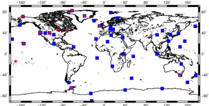
Fig. 1. Surface sites from the NOAA, ENEA, CSIRO, JMA and NIWA networks used in this study with red circles for surface sites observing MCF dry air mole fractions and blue squares for surface sites observing CH4
dry air mole fractions.
24
Fig. 1. Surface sites from the NOAA, ENEA, CSIRO, JMA and
NIWA networks used in this study with red circles for surface sites observing MCF dry air mole fractions and blue squares for surface sites observing CH4dry air mole fractions.
iteratively solved with the M1QN3 algorithm developed by Gilbert and Lemaréchal (1989) until the gradient norm gets reduced by more than 99 %. The inversion system provides the statistically-optimal solution, given the observations, the prior information and their respective uncertainties (i.e. the maximum of the posterior probability density function), but not directly the uncertainties associated with this solution. In fact, these uncertainties can be estimated by calculating the Hessian matrix but this is practically very costly given the dimension of the state vector. Instead, we use a robust Monte Carlo approach to compute the posterior uncertain-ties (Chevallier et al., 2007). This method involves perform-ing several inversions with randomly perturbed observations and priors according to their respective error statistics. Be-cause the estimation of the posterior uncertainties seems to become stable from 8 inversions (not shown), an ensemble of ten 19-month inversions (i.e. 190 members) is assumed to be enough to produce an ensemble of solutions well repre-senting the dispersion around the optimal solution xa. It
com-pletes the description of the posterior distribution for aggre-gated values (typically regional and annual). The improve-ment of methane emissions brought by an inversion is char-acterized by the uncertainty reduction, defined as one minus the ratio between posterior and prior uncertainties.
In addition to testing default configurations of the inver-sion system, we perform two sensitivity tests, which are de-fined as follows.
2.2 Bias correction
The first sensitivity test relies on a bias correction for some of the satellite retrievals. In a previous inversion study, Berga-maschi et al. (2009) proposed a bias correction as a function of the latitude and of the month for SCIAMACHY. Here, we parameterize possible biases of SCIAMACHY and TANSO-FTS as a function of the air mass factor AF. AFis a parameter
varying with the latitude as well, but it has the advantage of directly accounting for the geometrical position of the
ob-serving satellite and of the Sun.
AF=
1 cos(θ )+
1
cos(ξ ), (3)
where θ represents the solar zenith angle and ξ the viewing angle of the satellite. The optimized 4-D CH4state obtained
from the inversion using surface measurements is considered as our reference. We linearly regress the difference between this optimized state and the satellite observations of TANSO-FTS and SCIAMACHY against AF for the 19-month
pe-riod at once. With 2 parameters only, estimated from the 19 months of the reference inversion with seasonally-varying data coverage, we still consider our reference to be indepen-dent from the other inversions for the quantities studied in the following.
2.3 Tuning of error statistics
In our second sensitivity test, we use the method of Desroziers et al. (2006) to compute simple diagnostics about the error variances of the observations (diagonal of R matrix) and of the prior emissions (diagonal of B matrix) projected into the observation space. In principle, this method is an iter-ative process in which B and R are tuned from the following equations until convergence:
(HBHT)i+1=E[(H (xai) − H (xb))(y − H (xb))T] (4)
(R)i+1=E[(y − H (xia))(y − H (xb))T] (5)
(HBHT)i+1+(R)i+1=E[(y − H (xb))(y − H (xb))T] (6)
with i the iteration index within this process. Practically, this iterative process is very costly. In fact, Eqs. (4)–(6) require the implementation of the inversion, of which the error statis-tics are diagnosed, and the implementation of the complete Monte Carlo study associated (i.e. 10 more perturbed inver-sions see Sect. 2.1). In this study, only one iteration of these diagnostics is implemented for each inversion. Eqs (4)–(6) are applied here to the ensemble defined by all observations at once for the period June 2009–December 2010, i.e. by av-eraging the diagonals of the matrices described by both sides of the equations. By doing so, both sides are scalar values. These equations allow calculating the values diago, diagband diag respectively representing the diagnosed values for the observations, the prior and the full variances (right-hand side of the equations). From our initial inverse set-up, we com-pute the observation error variances (varo), the prior error
variances in the observation space (varb) and the sum of the
observation error variances and of the prior error variances, called the full variances hereinafter (var = varo+varb), that
are defined in our system (left-hand side of the equations).
(HBHT)i+1 (i.e. varb) is computed from the spread of a
Monte Carlo ensemble simulation, where each ensemble member is drawn from B. The ratio (ratio = diagvar) is an indi-cator of the goodness of the variances used in our inversions
and, in the best case, equals one. These diagnostics can be ad-vantageously extended to also tune the error correlations (off diagonal terms of R and B) and not only variances. However, this implies defining retrieval ensembles for each correlation lag, in spite of irregular spatiotemporal sampling; this is not attempted here.
2.4 Chemistry-transport model: LMDz-SACS
The inversion scheme includes a chemistry-transport model (CTM) that combines the LMDz4 transport model (Hourdin et al., 2006) in a nudged (towards analysed winds) and of-fline (transport mass fluxes are precomputed) mode, and the chemistry module SACS implemented by Pison et al. (2009) to estimate the methane emissions that most likely generated the observed mole fractions. The SACS module accounts for the interactions between CH4, OH and MCF. Indeed, MCF
only reacts with OH, which controls 90 % of the destruc-tion of CH4in the troposphere. Measurements of MCF mole
fractions, the emissions of which are relatively well known, are used as an additional constraint for the OH modelled mole fractions. CH4 and MCF mole fractions are
synergis-tically optimized during the inversion process to estimate the methane surface sources and the methane atmospheric sink on a spatial grid of 3.75◦×2.5◦and with a weekly temporal resolution.
3 Prior information and observations 3.1 Prior information
Our system exploits some prior information xbwhich
com-bines different standard and recent inventories (Table 1). The anthropogenic emissions of CH4are drawn from the
Emis-sion Database for Global Atmospheric Research EDGAR v4.2 (Olivier and Berdowski, 2001) and biomass burning emissions are from the interannual Global Fire and Emis-sion Database GFED3 (van der Werf et al., 2010), both valid for 2008. No effort is made here to adapt these inventories to the years of the study (2009 and 2010). Other sources are added to these emissions: termites from a study of Sander-son (1996), ocean from Lambert and Schmidt (1993) and wetlands from Kaplan (2002) which have been rescaled by P. Bergamaschi (personal communication, 2009). Soil uptake is based on Ridgwell et al. (1999). The 3-D concentrations of OH are obtained from a previous simulation of the full atmo-spheric chemistry model LMDz-INCA (Hauglustaine et al., 2004). MCF emissions are described by the EDGAR v3.2 database and are extrapolated for the years 2009 and 2010 based on a former atmospheric inversion (Bousquet et al., 2005), which has been updated.
Current bottom-up inventories range between 223 Tg yr−1 and 469 Tg yr−1 for the global methane natural sources and between 296 Tg yr−1and 353 Tg yr−1for the global methane anthropogenic sources (Kirschke et al., 2013), implying large
uncertainties of methane emissions. The standard deviation of the errors of grid-point weekly CH4 prior emissions are
defined here as a percentage (120 %) of the maximum value of the prior emissions between the 8 nearest neighbours in the corresponding month for each grid point (Pison et al., 2009). Errors on OH scaling factors are set at ±10 % and those on MCF are set at ±1 % of the flux (from now on, the ± sign is used to represent standard deviations). MCF er-rors are relatively small because their emissions are consid-ered to be well known, which motivates their use to constrain the OH concentrations. Errors on the initial conditions are set at ±10 % for MCF concentrations and ±3 % for CH4
con-centrations. All error spatial correlations are defined by an e-folding length of 500 km over land and of 1000 km over sea, without any correlation between land and ocean grid points. Temporal error correlations are all defined by an e-folding length of 2 weeks. Combining variances and correlations, the CH4prior emissions budget amounts to 554±51 Tg yr−1,
which is consistent with the large range seen among the cur-rent bottom-up inventories (Kirschke et al., 2013). This ini-tial B will be further tuned in a sensitivity test (Sect. 4.3) based on the objective diagnostics described in Sect. 2.3: a scalar factor α is estimated so that the new covariance ma-trix αB satisfies Eq. (4).
3.2 Surface measurements
Pointwise methane surface measurements are sparsely dis-tributed but provide observations of the dry air mole frac-tions with high accuracy and precision (0.2 %). We have se-lected 49 sites that had regular measurements during the pe-riod June 2009–December 2010 (Fig. 1) from the NOAA global cooperative air sampling network (Dlugokencky et al., 1994, 2009), JMA (Matsueda et al., 2004), ENEA (Artuso et al., 2007), CSIRO (Francey et al., 1999) and NIWA (Lowe et al., 1991) networks. The synoptic variability from NOAA’s GLOBALVIEW-CH4 (2009) is used as a proxy for transport error, which largely dominates the observation error. Over-all, observation standard deviations range from 3.4 ppb (sta-tion Casey, Australia) to 58.5 ppb (sta(sta-tion Tae-ahn Peninsula, Republic of Korea).
Methyl chloroform (MCF) is a molecule used in the past as an industrial solvent. Its use and emission have been re-stricted since the Montreal Protocol and its amendments so that its concentration has exponentially decreased in the last decades. Following Montzka et al. (2000, 2011), only flask data from the NOAA network are used in our inversions. Twelve sites have been selected over our study period; they are not homogeneously distributed (Fig. 1). During the in-version process, OH columns are scaled into 4 latitude bands to fit the MCF and CH4observations. In the southern
tropi-cal band, only Samoa Observatory (SMO) observes the MCF dry air mole fractions. SMO did not have a regular sam-pling, with no data between April and July 2010, implying that MCF does not add much constraint on the chemical
Table 1. Global annual prior methane emissions used in the inversions.
Emissions Tg yr−1 Source
Anthropogenic emissions 364 EDGAR v4.2, Olivier and Berdowski (2001) Biomass burning 14 GFED3, van der Werf et al. (2010)
Termites 20 Sanderson (1996)
Ocean 17 Lambert and Schmidt (1993)
Wetlands 177 Kaplan (2002) rescaled by P. Bergamaschi (personal communication, 2009)
Soil −38 Ridgwell et al. (1999)
Total 554
loss in this band. The MCF monthly variances are averaged over each year from NASA’s Advanced Global Atmospheric Gases Experiment (AGAGE) program (Prinn et al., 2005) when available, otherwise from the NOAA. These averages, representing synoptic variability, are used as MCF observa-tion errors. MCF standard deviaobserva-tions range from 0.07 ppt (station Summit, Denmark) to 0.21 ppt (station Harvard For-est Massachusetts, USA).
3.3 Satellite observations
SCIAMACHY was operated on board the European satel-lite ENVISAT between March 2002 and April 2012. It or-bited at 800 km and covered Earth in full every 6 days with a swath of 960 km and a ground resolution of 30 km (along track) and 60 km (across track) at nadir. The instrument ob-served the solar radiation reflected at the surface and the top of the atmosphere in the short wave infrared (SWIR) domain that allows deducing total columns of methane in cloud-free and sunlight conditions. The ratio of the CH4and
CO2dry air mole fractions is retrieved together with the
cor-responding averaging kernels using the Iterative Maximum A Posteriori (IMAPv55) DOAS (differential optical absorp-tion spectroscopy) algorithm initially detailed by Franken-berg et al. (2006). We use this ratio and the 4-D CO2
analy-sis from the surface air-sample inversion of Chevallier et al. (2010) to obtain the column-averaged dry air mole fraction of CH4(XCH4). The retrievals have a lower accuracy over
the oceans, where the reflection of the solar radiation is very weak and at high latitudes as well. To avoid biases that may be introduced by these data and following Bergamaschi et al. (2009), we limit our study to the observations over land within 50◦from the Equator and for which ground altitudes
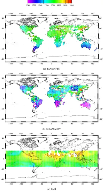
and model orography differ by less than 250 m. The selected XCH4 data (Fig. 2b) are then averaged (non-weighted by
their errors) into grid cells for each time step of the model so that “super-observations” are obtained. Lastly, we remove outliers by suppressing the super-observations whose depar-ture to the prior is larger than three times the standard de-viation of all departures. The mean of these averaged obser-vations is about 1747 ppb. The uncertainty of the XCH4
re-trievals is around 2 % (Frankenberg et al., 2006). Following Pison et al. (2009) and Spahni et al. (2011), a CTM error of 8 % of the observation values, describing the inability of the model to represent the observations and accounting for cor-related errors (see Sect. 2.1), is quadratically added to this retrieval error. In a sensitivity test (Sect. 4.3), a tuning will be computed based on the objective diagnostics described in Sect. 2.3: a scalar factor γ is estimated so that the new co-variance matrix of the observation errors γ R satisfies Eq. (5). The Japanese satellite GOSAT was launched in January 2009 and has a polar sun-synchronous orbit at 667 km. It provides a full coverage of Earth every 3 days with a swath of 750 km and a ground pixel resolution of 10.5 km at nadir. The TANSO-FTS instrument also observes in the SWIR do-main. Version 3.2 of the TANSO-FTS XCH4proxy retrievals
performed at the University of Leicester (Parker et al., 2011) are used with associated averaging kernels and a priori pro-files. The XCH4 retrieval algorithm uses an iterative
re-trieval scheme based on Bayesian optimal estimation. The retrieval accuracy is estimated to be about 0.6 %. As for SCIAMACHY, CO2columns at appropriate time and
loca-tion from Chevallier et al. (2010) are then used as a proxy for light path to retrieve the averaged mole fractions of methane. A CTM error of 8 % of the observation is quadratically added to this error (see previous paragraph). Given the similar-ity between SCIAMACHY and TANSO-FTS measurements, we apply the data selection of the previous paragraph (see Fig. 2a), create “super-observations” and remove outliers as well. The assimilated observations have a mean of 1775 ppb. Moreover, the covariance matrix for TANSO-FTS R will also be tuned with a scalar γ in Sect. 4.3.
The European MetOp-A satellite was launched in Octo-ber 2006 and has a polar sun-synchronous orbit at an al-titude of 817 km. On board MetOp-A, the Infrared Atmo-spheric Sounding Interferometer (IASI) measures the ther-mal radiation coming from Earth and the atmosphere in the thermal infrared domain (TIR) with a spectral resolu-tion of 0.5 cm−1 apodized. It provides a full global cov-erage daily with a swath of 1066 km and a ground reso-lution of 12 km at nadir. The retrieval algorithm is based on a non-linear inference scheme (Crevoisier et al., 2009,
(a) TANSO-FTS
(b) SCIAMACHY
(c) IASI
Fig. 2. Satellite ”super-observations” ( ppb) used in the inversions for the month of July 2010.Fig. 2. Satellite “super-observations” (ppb) used in the inversions25
for the month of July 2010.
2013). It allows inferring mid-to-upper troposphere columns of methane for the tropical band between 30◦S and 30◦N, in-cluding both land and ocean, twice a day at 09:30 a.m./p.m. local time, with an accuracy of 1.2 %. A CTM error of 3 % of the CH4mid-to-upper troposphere columns is quadratically
added to the retrieval error. The lower CTM error compared to TANSO-FTS and SCIAMACHY relates to the lesser verti-cal extent of the IASI (partial) column retrieval that does not include the boundary layer. IASI retrievals (Fig. 2c) are also averaged into super-observations and outliers are removed as well. This removal suppresses about 10 % of the super-observations which now have a mean of 1788 ppb. A tuning
of the observation error covariance matrix for IASI is done as for the other instruments in Sect. 4.3.
4 Results
A series of grid-point inversions covering the period from June 2009 to December 2010 are computed with the inverse model presented in Sect. 2 and the data sets presented in Sect. 3. To avoid edge effects, we study the methane emis-sions for the one-year period from August 2009 to July 2010. This time period has been chosen to have all observing sys-tems available. Posterior states given by the inversions are then aggregated at global or regional scales and evaluated at the local scale, i.e. at the surface sites. Each inversion will be called XXαγ with XX a two-letter code specific to each ob-serving system (SC for SCIAMACHY, TA for TANSO-FTS, IA for IASI and SU for surface sites) and α and γ the multi-plicative factors associated, respectively, with the covariance matrices B (see Sect. 3.1) and R (see Sect. 3.3).
4.1 Default configurations
For this first set of inversions, no tuning of inversions errors is performed. We present and analyse SU11, SC11, TA11 and IA11.
4.1.1 Global and regional budgets
Figure 3a presents the methane global annual emissions and losses as inferred by the inversions. When compared to the prior fluxes, the global emission budgets of TANSO-FTS (TA11) and SCIAMACHY (SC11) are respectively increased by 3.9 % (+22 Tg yr−1) and 4.2 % (+24 Tg yr−1) (see Table 3). They are decreased for IASI (IA11) and the surface (SU11) re-spectively by 2.3 % (−12 Tg yr−1) and 3.6 % (−19 Tg yr−1). Chemical losses are increased by 0.4 % (+2 Tg yr−1) for TA11 only. For the other observing systems, they are de-creased by 1.4 % (−8 Tg yr−1), 0.3 % (−2 Tg yr−1) and 3 % (−17 Tg yr−1) respectively for SC1 1, IA 1 1and SU 1 1. This leads
to global annual growth rates of +39 Tg yr−1, +51 Tg yr−1,
+9 Tg yr−1and +17 Tg yr−1respectively for TA11, SC11, IA11 and SU11. Uncertainty reductions on global budgets, esti-mated with a Monte Carlo approach as detailed in Sect. 2.1, are of 41 %, 51 %, 56 % and 60 % respectively for TA11, SC11, IA11 and SU11 (see Table 2). The global posterior un-certainty is inferred from the unun-certainty reduction and the global prior uncertainty of 51 Tg yr−1and completes the
de-scription of posterior global annual estimates of methane. The global emission budgets amount to 576 ± 30 Tg yr−1, 578 ± 25 Tg yr−1, 542 ± 22 Tg yr−1and 535 ± 20 Tg yr−1 re-spectively for TA11, SC11, IA11and SU11. As shown by Fig. 3a, with error bars representing the 1-sigma standard deviations (68 % of the posterior distribution), the global emissions and chemical losses of methane inferred from the different
(a)
(b)
Fig. 3. Global emissions (circles) and losses (triangles) for the configurations T A1
1(blue), SC11(red), IA11
(green) and SU1
1(violet) (a) and for T A11(dark blue), SC11(red) and bias-corrected configurations T A11CAF
(light blue) and SC1
1CAF(magenta) (b). Numbers describe the global growth rates in Tg yr−1inferred by the
inversions. Error bars represent the posterior uncertainties estimated with the Monte-Carlo study (see Section 2.1).
26
Fig. 3. Global emissions (circles) and losses (triangles) for the
con-figurations TA11(blue), SC11(red), IA11(green) and SU11(violet) (a) and for TA11 (dark blue), SC11(red) and bias-corrected configura-tions TA11CAF (light blue) and SC11CAF(magenta) (b). Numbers
describe the global growth rates in Tg yr−1inferred by the inver-sions. Error bars represent the posterior uncertainties estimated with the Monte Carlo study (see Section 2.1).
observing systems are statistically consistent with each other, in the sense that they agree within at least two sigmas.
The methane emissions are then aggregated over large continental regions (shown in Fig. 4a and adapted from Gur-ney et al., 2002). As shown by Fig. 4b, the three satellites show a very good agreement for 8 regions: North American Boreal, USA, South American Temperate, Southern Africa, West Europe, Eurasian Boreal, Middle East and Australia. In some of them (USA, South American Temperate, Southern Africa, West Europe, Eurasian Boreal and Middle East), this agreement combined with significant uncertainty reductions reflects a good improvement of our knowledge of methane emissions. For some other regions (North American Boreal and Australia), the inversion process infers marginal incre-ments and very weak uncertainty reductions for the three satellites, meaning that we do not really improve our knowl-edge of methane emissions for these regions. Large differ-ences are found between satellite- and surface-based inver-sions for regions USA, South American Temperate and South
(a)Sub-continental regions inspired from Gurney et al. (2002)
(b)
(c) Fig. 4. Regional methane emissions for default configurations T A1
1(blue), SC 1 1(red), IA 1 1(green) and SU 1
1(violet) (b) and for
configurations T A1
1(dark blue), SC11(red) and bias-corrected configurations T A11CAF(light blue) and SC11CAF(magenta) (c). Error
bars represent the posterior uncertainties estimated with the Monte-Carlo study (see Section 2.1).
27
Fig. 4. (a) Sub-continental regions inspired from Gurney et
al. (2002). Regional methane emissions for default configurations TA11(blue), SC11 (red), IA11(green) and SU11 (violet) (b) and for configurations TA11(dark blue), SC11(red) and bias-corrected con-figurations TA11CAF(light blue) and SC11CAF(magenta) (c). Error
bars represent the posterior uncertainties estimated with the Monte Carlo study (see Section 2.1).
East Asia. The surface-based inversion does not agree with the satellite ones, especially in the Tropics where there are few surface data. It seems that the increments found in re-gion USA by the surface-based inversion are highly overes-timated. Large differences between IASI and the other ob-serving systems are found in regions South East Asia and In-donesia. The IASI-based inversion achieves high uncertainty reductions for these regions (64 % in Indonesia and 51 % in South East Asia). However, the uncertainty reduction com-putation only accounts for random errors but biases in the transport model for this area may degrade the actual perfor-mance. Therefore, the differences are more likely due to a misattribution of the emissions in these regions because of a
Table 2. Uncertainty reduction (%) on methane emissions for the
default configurations.
Regions TA11 SC11 IA11 SU11 North American Boreal 07 00 00 41
USA 18 15 10 35
South American Tropical 21 31 48 16 South American Temperate 41 37 43 33 Northern Africa 53 61 63 49 Southern Africa 13 12 24 29 West Europe 15 16 04 51 East Europe 21 15 00 46 Eurasian Boreal 11 17 06 45 Middle East 30 24 07 13 South Asia 35 44 35 33 South East Asia 39 32 36 51 Australia 01 00 02 26 Indonesia 29 20 64 38
Global 41 51 56 60
larger footprint of the IASI free tropospheric column com-bined with a lack of retrievals during the monsoon period. 4.1.2 Initial conditions
2-D scaling factors adjust the initial conditions of CH4 and
MCF on 1 June 2009 at 00:00 UTC (see Sect. 3.1) and there-fore influence the mass budget of the inversion. After the in-versions SC11, TA11, IA11 and SU11, the initial CH4 columns
show increments of about 1.1±0.6 %, 0.7±0.6 %, 0.8±1.0 % and 0.8 ± 0.7 % respectively. The spatial distribution of these columns is very different between SCIAMACHY and the other observing systems. Figure 5b shows a decrease of the amplitude of the columns in the two hemispheres that can reach 3 % for SCIAMACHY, with a slight increase in the Tropics (less than 1 %). However, for TANSO-FTS, IASI and the surface sites, Fig. 5a, c, 6a show an increase especially located in the Southern Hemisphere that can reach 4 % for IASI, 3 % for TANSO-FTS and 2 % for the surface.
4.1.3 Fit to surface measurements
The fit to the surface data is summarized by the absolute mean of the biases (called mean bias hereinafter) and the root mean squares of the bias (called rms hereinafter) (last 2 columns of Table 3) between the posterior states ob-tained by using the different data sets, respectively TA11, SC11, IA11 and SU11, and their equivalent seen at each sur-face site (see Figs. 7a–c and 8a respectively). The mean bias obtained by TA11 is 4.1 ppb, which is well bellow the SC11 one (39.1 ppb) and the IA11 one (13.0 ppb), and close to the SU11one (0.8 ppb). The rms obtained by TA11is 15.4 ppb, the one by SC11is 40.5 ppb, the one by IA11is 20.0 ppb and the one by SU11 is 5.5 ppb. Note that for SU11, surface
observa-(a) T A1 1 (b) SC1 1 (c) IA1 1
Fig. 5. Increments of the initial conditions of methane for the various inversions expressed as a fraction of the prior.
28
Fig. 5. Increments of the initial conditions of methane for the
vari-ous inversions expressed as a fraction of the prior.
tions are assimilated by the inverse system, therefore explain-ing low rms and mean-bias values. Only the SCIAMACHY-based inversion does not result in improved agreement with surface measurements when compared to the prior mean bias (24.3 ppb) and rms (28.1 ppb).
(a) SU1 1 (b) T A1 1CAF (c) SC1 1CAF
Fig. 6. Increments of the initial conditions of methane for the various inversions expressed as a fraction of the prior. 29
Fig. 6. Increments of the initial conditions of methane for the
vari-ous inversions expressed as a fraction of the prior.
4.2 Bias correction
A bias correction as a function of the air mass factor AF(see
Sect. 2.2) is applied to TANSO-FTS and SCIAMACHY re-trievals, as presented in Sect. 3.3. SC11CAFand TA11CAF
rep-resent the inversions using bias-corrected satellite retrievals
(a) T A1 1 (b) SC1 1 (c) IA1 1
Fig. 7. Fit at surface sites (unitless) represented as the ratio of the posterior to the prior values of bias (in absolute values) between simulated and observed methane concentrations.
30
Fig. 7. Fit at surface sites (unitless) represented as the ratio of the
posterior to the prior values of bias (in absolute values) between simulated and observed methane concentrations.
of SCIAMACHY and TANSO-FTS respectively. As shown by Fig. 9a, b, the linear model is 4.0 × AF−34.0 ppb for
TANSO-FTS and 13.7 × AF−26.6 ppb for SCIAMACHY.
SC11CAFand TA11CAFare compared to SC11 and TA11 from
Sect. 4.1 to evaluate the impact of such a correction. 4.2.1 Global and regional budgets
At the global scale, as shown by Fig. 3b and Table 3, the bias correction decreases both posterior emissions and losses for TANSO-FTS respectively by 1 % (6 Tg yr−1) and 0.6 % (3 Tg yr−1), leading to a decrease of 7 % in the annual growth
(a) SU1 1 (b) T A1 1CAF (c) SC1 1CAF
Fig. 8. Fit at surface sites (unitless) represented as the ratio of the posterior to the prior values of bias (in absolute values) between simulated and observed methane concentrations.
31
Fig. 8. Fit at surface sites (unitless) represented as the ratio of the
posterior to the prior values of bias (in absolute values) between simulated and observed methane concentrations.
rate (36 Tg yr−1 instead of 39 Tg yr−1 without correction). For SCIAMACHY, the correction increases both posterior emissions and losses respectively by 0.7 % (4 Tg yr−1) and
0.2 % (2 Tg yr−1), leading to an increase of 6 % in the
an-nual growth rate (53 Tg yr−1 instead of 51 Tg yr−1 without correction). The correction induces increments of the same order of magnitude for the two satellites but these do not have the same signs. The bias correction in TANSO-FTS retrievals shows methane emissions, growth rates and fit to surface sites closer to the surface-based inversion ones. For SCIAMACHY, the correction does not improve the
agree-(a)
(b) Fig. 9. Linear regression for SU1
1 posterior state (Model) minus TANSO-FTS observations (a) or
SCIA-MACHY observations (b) as a function of the airmass factor (AF).
32
Fig. 9. Linear regression for SU11 posterior state (model) minus TANSO-FTS observations (a) or SCIAMACHY observations (b) as a function of the air mass factor (AF).
ment between the posterior state and the surface in terms of methane emissions and growth rates even though improves the fit to independent surface sites (see Fig. 8c and Table 3).
At the regional scale, when compared to the non-corrected inversion TA11, posterior methane emissions of TA11CAFare
slightly increased or decreased, getting closer to the ref-erence inversion for all regions. As shown by Fig. 4c, the emissions are increased especially in mid- and high-latitudes, such as in region East Europe (+13 %). They are decreased especially in the Tropics, such as in region Indone-sia (−7.6 %). For SCIAMACHY, the correction triggers in-creases or dein-creases following the reference increments for almost all regions, with exceptions particularly in regions South American Tropical (−4 %) and South American Tem-perate (+4 %). The correction only infers marginal variations of methane emissions and does not improve the agreement between SC11CAFand the surface-based inversion at the
re-gional scale. As surface measurements are especially located in mid- and high-latitudes, it makes sense that the largest in-consistencies with the reference concern the Tropics.
Table 3. Global emissions, chemical losses, growth rates of methane, fit to surface sites described by the absolute mean bias and rms. XXαγ
where XX is a two-letter code specific to each observing system (SC for SCIAMACHY, TA for TANSO-FTS, IA for IASI and SU for surface sites); α and γ are the multiplicative factors associated with the covariance matrices B (see Sect. 3.1) and R (see Sect. 3.3).
Name Emissions Loss Growth rate Mean bias Rms Tg yr−1 Tg yr−1 Tg yr−1 ppb ppb PRIOR 554 ± 51 535 ± 51 19 ± 50 24.3 28.1 SU11 535 ± 20 518 ± 51 17 ± 31 0.8 5.5 TA11 576 ± 30 537 ± 51 39 ± 38 4.1 15.4 SC11 578 ± 25 527 ± 51 51 ± 36 39.1 40.5 IA11 542 ± 22 533 ± 51 9 ± 35 13.0 20.0 TA11CAF 570 ± 30 534 ± 51 36 ± 23 2.7 13.7 SC11CAF 582 ± 25 529 ± 51 53 ± 22 23.4 26.4 SU0.61 538 ± 15 519 ± 30 19 ± 24 9.1 10.3 TA0.60.075 565 ± 21 537 ± 30 28 ± 25 2.2 16.1 SC0.60.2 631 ± 16 549 ± 30 83 ± 28 39.7 44.3 IA0.60.22 530 ± 16 530 ± 30 0 ± 20 15.5 23.6 TA1.50.075 568 ± 29 541 ± 71 27 ± 48 1.9 15.2 IA1.50.22 549 ± 36 536 ± 71 13 ± 50 12.4 19.2 4.2.2 Initial conditions
The initial columns of the two configurations using TANSO-FTS observations have the same spatial distribution. How-ever, the bias correction infers larger negative increments in the Northern Hemisphere and weaker positive increments in the Southern Hemisphere. The intial columns of the two con-figurations of SCIAMACHY are dominated by a strong de-crease compared to the prior (see Fig. 6c) with the largest negative variations (around 3 %) located in the Northern Hemisphere. The CH4 initial columns vary by 1.1 ± 0.6 %
without correction (SC11) and by 0.8 ± 0.5 % with the bias correction (SC11CAF). The bias correction seems to make the
spatial distribution of the SC11CAF initial conditions agree
more with TA11or TA11CAFinitial conditions (Figs. 5a, 6b),
which show a positive anomaly in the Tropics of the Southern Hemisphere.
4.2.3 Fit to surface measurements
For TANSO-FTS, the mean bias between the model and the surface observations is decreased from 4.1 ppb to 2.7 ppb (see Table 3) and the rms is slightly reduced from 15.4 ppb to 13.7 ppb after the bias correction. The bias correction marginally improves the fit to surface sites in the Northern Hemisphere where five more sites show better agreement be-tween surface measurements and the posterior state of the
corrected version TA11CAF(Fig. 8b). For SCIAMACHY, the
fit to the surface sites is slightly improved in the mid-latitudes and better in the Tropics (see Figs. 7b and 8c). The bias correction improves the fit for 10 sites located in the two hemispheres while the mean bias is reduced from 39.1 ppb to 23.4 ppb and the rms is reduced from 40.5 ppb to 26.4 ppb but still not better than the prior (mean bias = 24.3 ppb and rms = 28.1 ppb).
4.3 Tuning of error statistics
4.3.1 Diagnostics on default configurations
The results of the diagnostics introduced in Sect. 2.3 and ap-plied to the default configurations SU11, SC11, TA11 and IA11 are presented in Table 4. They suggest that prior error vari-ances are overestimated by almost 2-fold for the surface (ratiob= 1.68) and SCIAMACHY (ratiob= 1.82) while they
are underestimated by 1.5 for TANSO-FTS (ratiob= 0.64)
and IASI (ratiob= 0.69). The differences among prior error
diagnostics for the four observing systems likely stems from the use of a single scaling factor for the whole matrix that may have a more complex structure in reality. Each observ-ing system suggests a scalobserv-ing factor in this context, based on its own spatial and temporal sensitivity.
The observation errors seem to be fairly well repre-sented in our system for the surface (ratioo= 0.79) even
(a)
(b)
Fig. 10. Global emissions (circles) and losses (triangles) (a) and regional emissions (b) for the ”optimal” configurations T A0.6
0.075(blue), IA0.60.22(green) and SU10.6(violet). Numbers describe the global growth rates
in Tg yr−1inferred by the inversions. Error bars represent either the prior uncertainties (α = 0.6 in black and
α = 1.5 in dark green), either the posterior uncertainties estimated with the Monte-Carlo study (see Section 2.1).
33
Fig. 10. Global emissions (circles) and losses (triangles) (a) and
regional emissions (b) for the “optimal" configurations T A0.60.075 (blue), I A0.60.22 (green) and SU10.6 (violet). Numbers describe the global growth rates in Tg yr−1 inferred by the inversions. Error bars represent either the prior uncertainties (α = 0.6 in black and
α =1.5 in dark green) or the posterior uncertainties estimated with the Monte Carlo study (see Sect. 2.1).
(ratioo= 13.69), by 5-fold for SCIAMACHY (ratioo= 5.00)
and by 4-fold for IASI (ratioo= 4.41). The initial value of
ratioofor the satellites is related to our use of a diagonal R,
with inflated variances qualitatively compensating for miss-ing correlations (see Sect. 2.1). It should be noted that the diagnostics do not account for this numerical artifact.
The full variances are slightly overestimated for the sur-face (ratio = 1.54) while they are overestimated by 4-fold for TANSO-FTS and SCIAMACHY (ratio = 4.24 for TA11 and ratio = 4.60 for SC11) and by 2-fold for IASI (ratio = 2.12 for IA11).
From these diagnostics, we perform two tuning experi-ments series where we tune observation and prior error vari-ances. We evaluate the results based on their agreement with our reference system, i.e. the surface network.
Table 4. Ratios (unitless) of the observation (ratioo), prior (ratiob)
and full (ratio) variances inferred from the diagnostics presented in Sect. 2.3. These quantities are respectively defined as the ratios be-tween prescribed (varo, varband var = varo+varb) and associated
diagnosed (diago, diagband diag) error variances and represent the goodness of the error statistics in the inversion system. Good statis-tical consistency is obtained when the ratios are close to 1.
NAME ratioo ratiob ratio
SU11 0.79 1.68 1.54 TA11 13.69 0.64 4.24 SC11 5.00 1.82 4.60 IA11 4.41 0.69 2.12 SU0.61 0.74 0.94 0.90 TA0.60.075 1.17 0.38 0.49 SC0.60.2 1.06 0.93 1.03 IA0.60.22 1.00 0.41 0.58 TA1.50.075 1.11 0.95 0.96 IA1.50.22 1.00 1.01 1.00 4.3.2 Tuning experiments 1
In the first experiment, we select the prior error variance (α = 0.6 = 1/1.68) suggested by our reference observing sys-tem (SU11). It avoids making the prior error matrix vary with the observing system. For the satellites, the observation er-rors are tuned in order to satisfy Eq. (5). For the surface, the observation error variances are not tuned as they are rather good already (ratioo= 0.79 for SU11). This tuning improves
all diagnostics for the surface (ratioo= 0.74, ratiob= 0.94
and ratio = 0.90 for SU0.61 see Table 4) and SCIAMACHY (ratioo= 1.06, ratiob= 0.93 and ratio = 1.03 for SC0.60.2) but
does not improve the agreement with the reference in terms of mole fractions (see Table 3). For the surface, the fit to as-similated surface sites is degraded. This result is expected as decreasing prior errors limits the possibility of the inversion to deviate from the prior to better fit the assimilated obser-vations. For SCIAMACHY, there is no real improvement of the fit to surface sites after inversion in terms of mean bias (39.7 ppb) and rms (44.3 ppb) when compared to the prior statistics of the bias. This suggests that the observation er-ror variances of SCIAMACHY have a more complex struc-ture than the one tuned here. Otherwise, the observation error diagnostics for TANSO-FTS (ratioo= 1.17 for TA0.60.075) and
IASI (ratioo= 1.00 for IA0.60.22) are both improved while the
prior error diagnostics are degraded for both satellite instru-ments (ratiob= 0.38 for TA0.60.075and ratiob= 0.41 for IA0.60.22),
confirming the fact that the prior error configuration satis-fying for the surface does not fit TANSO-FTS and IASI.
However, the agreement with independent surface sites is improved in terms of mean bias (2.2 ppb) for TANSO-FTS only (the rms is stable at 16.1 ppb) and is degraded for IASI (mean bias = 15.5 ppb and rms = 23.6 ppb).
4.3.3 Tuning experiments 2
In the second experiment, we tune both prior and obser-vation error variances following the diagnostics specific to TANSO-FTS and IASI. As suggested by the diagnostics ap-plied on the default configurations, we set α = 1.5 for prior errors (ratiob= 0.64 for TANSO-FTS and ratiob= 0.69 for
IASI) and the observation errors are independently tuned (ratioo= 13.69 for TANSO-FTS and ratioo= 4.41 for IASI).
The results of the diagnostics for the configurations TA1.50.075 and IA1.50.22are presented in Table 4. They suggest that all er-ror variances are fairly well prescribed in our system now (ratio = 0.96 for TA1.50.075and ratio = 1.00 for IA1.50.22). The fit to surface sites are improved by this tuning in terms of mean bias and rms for both instruments when compared to the default configurations (i.e. when α = γ = 1; see Table 3). However, for TANSO-FTS, the mean bias and rms are sim-ilar to the ones obtained by the first tuning experiment with prior error diagnostics degraded (i.e. configuration TA0.60.075), meaning that prior error variances have a minor effect on the quality of the inverted fluxes for this instrument. This is not the case for IASI, for which the prior error configuration has a larger impact on the inverted fluxes. When compared to the first experiment (i.e. IA0.60.22), the growth rate obtained for IASI is increased by 13 Tg yr−1, better agreeing with the
surface-based inversions while the fit to surface sites is also improved (mean bias = 12.4 ppb and rms = 19.2 ppb).
5 Discussion
The two satellite instruments observing in the SWIR do-main, TANSO-FTS and SCIAMACHY, infer larger emis-sions than the other two observing systems, respectively by
+41 Tg yr−1and +43 Tg yr−1for the default configurations (i.e. with α = γ = 1), when compared to the surface global budget of 535 Tg yr−1. This overestimation can be partly ex-plained by a bias identified as a function of the air mass factor in the satellite products, respectively of 4.0 × AF−34.0 ppb
and 13.7 × AF−26.6 ppb. Correcting this bias improves the
agreement between TANSO-FTS and the surface at global and regional scales and the fit to surface measurements as well. However, given the modesty of the bias and the un-certainty of the linear regression, its need is not obvious. For SCIAMACHY, the bias correction has a slight impact on the inverted methane emissions and does not improve the agreement with the surface at global and regional scales. It has a larger impact on the fit to surface measurements in terms of mole fractions, which is well improved when com-pared to the default configuration. However, for the
bias-corrected configuration SC11CAF, the mean bias (23.4 ppb)
and rms (26.4 ppb) are slightly improved by this inversion, when compared to the prior ones, but remain large. Such a correction is needed for SCIAMACHY, albeit not sufficient to reconcile the posterior state with the reference.
When comparing configuration TA1.50.075with the other test configuration (e.g. TA0.60.075), the fit to surface sites is sim-ilar since mean bias and rms are very close. The two sets of tuning experiments indicate that the information inferred from TANSO-FTS is robust in our system in terms of mole fractions and growth rates. IASI seems to be more sensi-tive to prior error assignment as methane emissions vary by 19 Tg yr−1 and growth rates by 13 Tg yr−1 among all sen-sitivity tests. Indeed, with a tuning specific to this satellite instrument, one gets a stable agreement with independent surface sites. Based on the fit to surface measurements, the inversions TA0.60.075and IA1.50.22are taken as optimal configura-tions obtained from the tuning procedure. The corresponding emission and loss budgets are summarized in Fig. 10. For all SCIAMACHY sensitivity tests, the mean bias and rms are worse than the prior ones, meaning that the inversion pro-cess does not improve the agreement with the surface mea-surements for this satellite. It seems that SCIAMACHY can-not agree with the reference by simply adjusting mean prior and observation error variances. This points to a complicated structure of the retrieval errors, at least for the period studied, possibly linked to the progressive degradation of the instru-ment. Direct conclusions regarding SCIAMACHY for earlier time periods cannot be drawn from our study, which focuses on years 2009–2010, the only overlap period between SCIA-MACHY and GOSAT.
For all observing systems, the largest emissions are located in region South American Tropical and may be explained by methane emissions from wetlands and from biomass burn-ing further to the severe drought in Amazonia in 2010. Large emissions are inferred as well in region South Africa, which are probably also caused by biomass burning. IASI differs from the other two observing systems in some regions. An overestimation of the emissions (when compared to the ref-erence) in Indonesia compensates an underestimation of the emissions in Asia, suggesting a misattribution of the emis-sions in these regions likely due to the large footprint of the mid-to-upper tropospheric column combined with a lack of retrievals during the monsoon period, i.e. between June and September. Another underestimation of the emissions in re-gion South American Tropical is seen as well, also due to a lack of IASI retrievals over this region between November 2009 and March 2010. This does not allow inferring the high emissions found by TANSO-FTS and the surface data during the drought of 2010.
The three observing systems (TANSO-FTS, IASI and the surface sites) still show good consistency in terms of emissions, meaning we can trust the main information re-trieved from them. However, in the Southern Hemisphere
the fit is not improved for the sites optimized during the surface-based inversions. Interestingly, we found a similar problem when inverting CO emissions from the Measure-ments Of Pollution In The Troposphere (MOPITT) on board NASA’s Terra satellite (Fortems-Cheiney et al., 2011). These two results may be partly explained by the too small ex-change time of this version of the LMDz transport model from the Northern Hemisphere to the Southern Hemisphere (Patra et al., 2011), which likely induces an artificial increase of the sources inferred in the North and an increase of the loss in the South to match the surface observations.
6 Conclusion
Using objective tuning methods for the error statistics, we show that one can achieve improved consistency between CH4emission and loss inferred from different observing
sys-tems. An exception is SCIAMACHY, which seems to be par-ticularly difficult to exploit over the period 2009–2010. The tuned covariance matrix is more optimistic about the quality of the prior fluxes than our initial estimates when assimilat-ing the global TANSO-FTS or the global surface network, whereas it is more conservative when assimilating the trop-ical IASI data. The observation error, initially set at around 8 % for TANSO-FTS and around 3 % for IASI, is reduced by 13-fold for TANSO-FTS and by 4-fold for IASI. The global TANSO-FTS, IASI and surface data budgets from the improved configurations are respectively 565 ± 21 Tg yr−1, 549 ± 36 Tg yr−1and 538 ± 15 Tg yr−1for the period August 2009–July 2010. To assess the current methane budget with TANSO-FTS, IASI and the surface sites, one can keep one or two of these observing systems out of the inversion for in-dependent evaluation, as we propose here. Alternatively, one can combine them together to better reduce uncertainties in the methane cycle, provided the tuning of the prior error is regionalized.
Acknowledgements. The first author is funded by CNES and CEA.
This work was performed using HPC resources from DSM-CCRT and [CCRT/CINES/IDRIS] under the allocation 2012-t2012012201 made by GENCI (Grand Equipement National de Calcul Intensif). We also thank the computing support team of the LSCE led by F. Marabelle. We aknowledge the contributors to the World Data Center for Greenhouse Gases for providing their data of methane and methyl-chloroform atmospheric mole fractions. The authors thank in particular S. Piacentino (ENEA), T. Kawasato (JMA) and S. Nichol (NIWA). NOAA authors receive partial funding for their measurements and research from the Atmospheric Chemistry, Carbon Cycle, and Climate (AC4) Program.
Edited by: A. Pozzer
The publication of this article is financed by CNRS-INSU.
References
Artuso, F., Chamard, P., Piacentino, S., Di Sarra, A., Meloni, D., Monteleone, F., Sferlazzo, D. M., and Thiery, F.: Atmospheric methane in the Mediterranean: analysis of measurements at the island of Lampedusa during 1995–2005, Atmos. Environ., 41, 3877–3888, doi:10.1016/j.atmosenv.2007.01.024, 2007. Bergamaschi, P., Frankenberg, C., Meirink, J. F., Krol, M.,
Vil-lani, M. G., Houweling, S., Dentener, F., Dlugokencky, E. J., Miller, J. B., Gatti, L. V., Engel, A., and Levin, I.: Inverse modeling of global and regional CH4 emissions using SCIA-MACHY satellite retrievals, J. Geophys. Res. Atmos., 114, D22301, doi:10.1029/2009JD012287, 2009.
Bergamaschi, P., Krol, M., Meirink, J. F., Dentener, F., Segers, A., van Aardenne, J., Monni, S., Vermeulen, A. T., Schmidt, M., and Ramonet, M.: Inverse modeling of European CH4
emissions 2001–2006, J. Geophys. Res. Atmos., 115, D22309, doi:10.1029/2010JD014180, 2010.
Bocquet, M., Wu, L., and Chevallier, F.: Bayesian design of control space for optimal assimilation of observations. Part I: Consis-tent multiscale formalism, Q. J. Roy. Meteorol. Soc., 137, 1340– 1356, doi:10.1002/qj.837, 2011.
Bousquet, P., Hauglustaine, D. A., Peylin, P., Carouge, C., and Ciais, P.: Two decades of OH variability as inferred by an in-version of atmospheric transport and chemistry of methyl chlo-roform, Atmos. Chem. Phys., 5, 2635–2656, doi:10.5194/acp-5-2635-2005, 2005.
Bousquet, P., Ciais, P., Miller, J. B., Dlugokencky, E. J., Hauglus-taine, D. A., Prigent, C., Werf, G. R. V. d., Peylin, P., Brunke, E.-G., Carouge, C., Langenfelds, R. L., Lathière, J., Papa, F., Ramonet, M., Schmidt, M., Steele, L. P., Tyler, S. C., and White, J.: Contribution of anthropogenic and natural sources to atmospheric methane variability, Nature, 443, 439–443, doi:10.1038/nature05132, 2006.
Bousquet, P., Ringeval, B., Pison, I., Dlugokencky, E. J., Brunke, E.-G., Carouge, C., Chevallier, F., Fortems-Cheiney, A., Franken-berg, C., Hauglustaine, D. A., Krummel, P. B., Langenfelds, R. L., Ramonet, M., Schmidt, M., Steele, L. P., Szopa, S., Yver, C., Viovy, N., and Ciais, P.: Source attribution of the changes in atmospheric methane for 2006–2008, Atmos. Chem. Phys., 11, 3689–3700, doi:10.5194/acp-11-3689-2011, 2011.
Chapnik, B., Desroziers, G., Rabier, F., and Talagrand, O.: Diagno-sis and tuning of observational error in a quasi-operational data assimilation setting, Q. J. Roy. Meteorol. Soc., 132, 543–565, doi:10.1256/qj.04.102, 2006.
Chen, Y.-H. and Prinn, R. G.: Estimation of atmospheric methane emissions between 1996 and 2001 using a three-dimensional global chemical transport model, J. Geophys. Res. Atmos., 111, D10307, doi:10.1029/2005JD006058, 2006.
Chevallier, F.: Impact of correlated observation errors on inverted CO2 surface fluxes from OCO measurements, Geophys. Res. Lett., 34, L24804, doi:10.1029/2007GL030463, 2007.
Chevallier, F., Fisher, M., Peylin, P., Serrar, S., Bousquet, P., Bréon, F. M., Chédin, A., and Ciais, P.: Inferring CO2 sources and sinks from satellite observations: Method and application to TOVS data, J. Geophys. Res., 110, D24309, doi:10.1029/2005JD006390, 2005.
Chevallier, F., Bréon, F. M., and Rayner, P. J.: Contribution of the Orbiting Carbon Observatory to the estimation of CO2 sources and sinks: Theoretical study in a variational data assimilation framework, J. Geophys. Res., 112, D09307, doi:10.1029/2006JD007375, 2007.
Chevallier, F., Feng, L., Bösch, H., Palmer, P. I., and Rayner, P. J.: On the impact of transport model errors for the estimation of CO2 surface fluxes from GOSAT observations, Geophys. Res.
Lett., 37, L21803, doi:10.1029/2010GL044652, 2010.
Crevoisier, C., Nobileau, D., Fiore, A. M., Armante, R., Chédin, A., and Scott, N. A.: Tropospheric methane in the tropics – first year from IASI hyperspectral infrared observations, Atmos. Chem. Phys., 9, 6337–6350, doi:10.5194/acp-9-6337-2009, 2009. Crevoisier, C., Nobileau, D., Armante, R., Crépeau, L., Machida, T.,
Sawa, Y., Matsueda, H., Schuck, T., Thonat, T., Pernin, J., Scott, N. A., and Chédin, A.: The 2007–2011 evolution of tropical methane in the mid-troposphere as seen from space by MetOp-A/IASI, Atmos. Chem. Phys., 13, 4279–4289, doi:10.5194/acp-13-4279-2013, 2013.
Desroziers, G., Berre, L., Chapnik, B., and Poli, P.: Diagnosis of observation, background and analysis-error statistics in ob-servation space, Q. J. Roy. Meteorol. Soc., 131, 3385–3396, doi:10.1256/qj.05.108, 2006.
Dlugokencky, E. J., Steele, L. P., Lang, P. M., and Masarie, K. A.: The growth rate and distribution of atmospheric methane, J. Geo-phys. Res. Atmos., 99, 17021–17043, doi:10.1029/94JD01245, 1994.
Dlugokencky, E. J., Bruhwiler, L., White, J. W. C., Emmons, L. K., Novelli, P. C., Montzka, S. A., Masarie, K. A., Lang, P. M., Crotwell, A. M., Miller, J. B., and Gatti, L. V.: Observational constraints on recent increases in the atmospheric CH4 burden, Geophys. Res. Lett., 36, L18803, doi:10.1029/2009GL039780, 2009.
Forster, P.: Changes in Atmospheric Constituents and in Radiative Forcing, Cambridge University Press, United Kingdom and New York, NY, USA, 129–234, 2007.
Fortems-Cheiney, A., Chevallier, F., Pison, I., Bousquet, P., Szopa, S., Deeter, M. N., and Clerbaux, C.: Ten years of CO emissions as seen from Measurements of Pollution in the Troposphere (MOPITT), J. Geophys. Res., 116, D05304, doi:10.1029/2010JD014416, 2011.
Francey, R. J., Steele, L. P., Langenfelds, R. L., and Pak, B. C.: High precision long-term monitoring of radiatively active and related trace gases at surface sites and from aircraft in the Southern Hemisphere atmosphere, J. Atmos. Sci., 56, 279–285, doi:10.1175/1520-0469(1999)056<0279:HPLTMO>2.0.CO;2, 1999.
Frankenberg, C., Meirink, J. F., Bergamaschi, P., Goede, A. P. H., Heimann, M., Körner, S., Platt, U., Weele, M. v., and Wagner, T.: Satellite chartography of atmospheric methane from SCIAMACHY on board ENVISAT: Analysis of the years 2003 and 2004, J. Geophys. Res., 111, D07303, doi:10.1029/2005JD006235, 2006.
Gilbert, J. C. and Lemaréchal, C.: Some numerical experiments with variable-storage quasi-Newton algorithms, Mathematical programming, 45, 407–435, doi:10.1007/BF01589113, 1989. GLOBALVIEW-CH4: Cooperative Atmospheric Data Integration
Project – Methane, CD-ROM, NOAA ESRL, Boulder, Colorado, 2009.
Gurney, K. R., Law, R. M., Denning, A. S., Rayner, P. J., Baker, D., Bousquet, P., Bruhwiler, L., Chen, Y.-H., Ciais, P., and Fan, S.: Towards robust regional estimates of CO2 sources and sinks using atmospheric transport models, Nature, 415, 626–630, doi:10.1038/415626a, 2002.
Hauglustaine, D., Hourdin, F., Jourdain, L., Filiberti, M., Wal-ters, S., Lamarque, J., and Holland, E.: Interactive chem-istry in the Laboratoire de Météorologie Dynamique gen-eral circulation model: Description and background tropo-spheric chemistry evaluation, J. Geophys. Res., 109, D04314, doi:10.1029/2003JD003957, 2004.
Hourdin, F., Musat, I., Bony, S., Braconnot, P., Codron, F., Dufresne, J.-L., Fairhead, L., Filiberti, M.-A., Friedlingstein, P., and Grandpeix, J.-Y.: The LMDZ4 general circulation model: cli-mate performance and sensitivity to parametrized physics with emphasis on tropical convection, Clim. Dynam., 27, 787–813, doi:10.1007/s00382-006-0158-0, 2006.
Houweling, S., Kaminski, T., Dentener, F., Lelieveld, J., and Heimann, M.: Inverse modeling of methane sources and sinks using the adjoint of a global transport model, J. Geophys. Res., 104, 26137–26160, doi:10.1029/1999JD900428, 1999.
Kaminski, T., Rayner, P. J., Heimann, M., and Enting, I. G.: On ag-gregation errors in atmospheric transport inversions, J. Geophys. Res. Atmos., 106, 4703–4715, doi:10.1029/2000JD900581, 2001.
Kaplan, J. O.: Wetlands at the Last Glacial Maximum: Distribu-tion and methane emissions, Geophys. Res. Lett., 29, 3-1–3-4, doi:10.1029/2001GL013366, 2002.
Kirschke, S., Bousquet, P., Ciais, P., Saunois, M., Canadell, J. G., Dlugokencky, E. J., Bergamaschi, P., Bergmann, D., Blake, D. R., and Bruhwiler, L.: Three decades of global methane sources and sinks, Nature Geosci., 6, 813–823, doi:10.1038/ngeo1955, 2013. Lambert, G. and Schmidt, S.: Reevaluation of the oceanic flux of methane: Uncertainties and long term variations, Chemosphere, 26, 579–589, doi:10.1016/0045-6535(93)90443-9, 1993. Lowe, D. C., Brenninkmeijer, C. A. M., Tyler, S. C., and
Dlugkencky, E. J.: Determination of the isotopic composition of atmospheric methane and its application in the Antarctic, J. Geo-phys. Res. Atmos., 96, 15455–15467, doi:10.1029/91JD01119, 1991.
Matsueda, H., Sawa, Y., Wada, A., Inoue, H. Y., Suda, K., Hirano, Y., Tsuboi, K., and Nishioka, S.: Methane standard gases for at-mospheric measurements at the MRI and JMA and intercom-parison experiments, Papers Meteorol. Geophys., 54, 91–113, doi:10.2467/mripapers.54.91, 2004.
Meirink, J. F., Bergamaschi, P., and Krol, M. C.: Four-dimensional variational data assimilation for inverse modelling of atmospheric methane emissions: method and comparison with synthesis inversion, Atmos. Chem. Phys., 8, 6341–6353, doi:10.5194/acp-8-6341-2008, 2008.
Montzka, S. A., Spivakovsky, C. M., Butler, J. H., Elkins, J. W., Lock, L. T., and Mondeel, D. J.: New observational constraints
for atmospheric hydroxyl on global and hemispheric scales, Sci-ence, 288, 500–503, doi:10.1126/science.288.5465.500, 2000. Montzka, S. A., Krol, M., Dlugokencky, E., Hall, B., Jöckel, P., and
Lelieveld, J.: Small interannual variability of global atmospheric hydroxyl, Science, 331, 67–69, doi:10.1126/science.1197640, 2011.
Olivier, J. G. J. and Berdowski, J. J. M.: Global emission sources and sinks, 2001.
Parker, R., Boesch, H., Cogan, A., Fraser, A., Feng, L., Palmer, P. I., Messerschmidt, J., Deutscher, N., Griffith, D. W. T., Notholt, J., Wennberg, P. O., and Wunch, D.: Methane observations from the Greenhouse Gases Observing SATellite: Comparison to ground-based TCCON data and model calculations, Geophys. Res. Lett., 38, L15807, doi:10.1029/2011GL047871, 2011.
Patra, P. K., Houweling, S., Krol, M., Bousquet, P., Belikov, D., Bergmann, D., Bian, H., Cameron-Smith, P., Chipperfield, M. P., and Corbin, K.: TransCom model simulations of CH 4 and re-lated species: linking transport, surface flux and chemical loss with CH 4 variability in the troposphere and lower stratosphere, Atmos. Chem. Phys., 11, 12813–12837, doi:10.5194/acp-11-12813-2011, 2011.
Pison, I., Bousquet, P., Chevallier, F., Szopa, S., and Hauglus-taine, D.: Multi-species inversion of CH4, CO and H2emissions
from surface measurements, Atmos. Chem. Phys., 9, 5281–5297, doi:10.5194/acp-9-5281-2009, 2009.
Prinn, R. G., Huang, J., Weiss, R. F., Cunnold, D. M., Fraser, P. J., Simmonds, P. G., McCulloch, A., Harth, C., Reimann, S., Salameh, P., O’Doherty, S., Wang, R. H. J., Porter, L. W., Miller, B. R., and Krummel, P. B.: Evidence for variability of atmo-spheric hydroxyl radicals over the past quarter century, Geophys. Res. Lett., 32, L07809, doi:10.1029/2004GL022228, 2005.
Ridgwell, A. J., Marshall, S. J., and Gregson, K.: Consumption of atmospheric methane by soils: A process-based model, Global Biogeochem. Cy., 13, 59–70, doi:10.1029/1998GB900004, 1999.
Rigby, M., Prinn, R. G., Fraser, P. J., Simmonds, P. G., Lan-genfelds, R. L., Huang, J., Cunnold, D. M., Steele, L. P., Krummel, P. B., Weiss, R. F., O’Doherty, S., Salameh, P. K., Wang, H. J., Harth, C. M., Mühle, J., and Porter, L. W.: Re-newed growth of atmospheric methane, Geophys. Res. Lett., 35, L22805, doi:10.1029/2008GL036037, 2008.
Sanderson, M. G.: Biomass of termites and their emissions of methane and carbon dioxide: A global database, Global Bio-geochem. Cy., 10, 543–557, doi:10.1029/96GB01893, 1996. Spahni, R., Wania, R., Neef, L., van Weele, M., Pison, I., Bousquet,
P., Frankenberg, C., Foster, P. N., Joos, F., Prentice, I. C., and van Velthoven, P.: Constraining global methane emissions and uptake by ecosystems, Biogeosciences, 8, 1643–1665, doi:10.5194/bg-8-1643-2011, 2011.
van der Werf, G., Randerson, J. T., Giglio, L., Collatz, G. J., Mu, M., Kasibhatla, P. S., Morton, D. C., DeFries, R. S., Jin, Y. v., and Leeuwen, T. v.: Global fire emissions and the contribution of deforestation, savanna, forest, agricultural, and peat fires (1997– 2009), Atmos. Chem. Phys., 10, 11707–11735, doi:10.5194/acp-10-11707-2010, 2010.