HAL Id: hal-00286065
https://hal.archives-ouvertes.fr/hal-00286065
Preprint submitted on 17 Jun 2008HAL is a multi-disciplinary open access
archive for the deposit and dissemination of sci-entific research documents, whether they are pub-lished or not. The documents may come from teaching and research institutions in France or abroad, or from public or private research centers.
L’archive ouverte pluridisciplinaire HAL, est destinée au dépôt et à la diffusion de documents scientifiques de niveau recherche, publiés ou non, émanant des établissements d’enseignement et de recherche français ou étrangers, des laboratoires publics ou privés.
optimal pruned K-nearest neighbors: op-knn application
to financial modeling
Eric Severin, Yoan Miche, Amaury Lendasse, Anti Sorjamaa, Qi Yu
To cite this version:
Eric Severin, Yoan Miche, Amaury Lendasse, Anti Sorjamaa, Qi Yu. optimal pruned K-nearest neighbors: op-knn application to financial modeling. 2008. �hal-00286065�
Qi Yu, Antti Sorjamaa, Yoan Miche, Eric S´everin∗ and Amaury Lendasse Helsinki University of Technology
Information and Computer Science Department Espoo, Finland
∗Associate Professor, Laboratoire Economie Management (LEM),
avenue du peuple Belge 59043 Lille cedex
Abstract - The paper proposes a methodology called OP-KNN, which builds a one hidden-layer feedforward neural network, using nearest neighbors neurons with extremely small com-putational time. The main strategy is to select the most relevant variables beforehand, then to build the model using KNN kernels. Multiresponse Sparse Regression (MRSR) is used as the second step in order to rank each kth nearest neighbor and finally as a third step
Leave-One-Out estimation is used to select the number of neighbors and to estimate the generalization performances. This new methodology is tested on a toy example and is applied to financial modeling.
Key words - Variable selection, k-Nearest Neighbors, Multiresponse Sparse Re-gression, Leave-One-Out, Financial Modeling
1
Introduction
It is usual to have very long computational time for training a feedforward network using existing classic learning algorithms even for simple problems. Thus, Guang-Bin Huang in his paper [1] proposed an original algorithm called Extreme Learning Machine (ELM) for single-hidden layer feedforward neural networks (SLFN) which randomly chooses single-hidden nodes and analytically determines the output weights of SLFNs. The most significant characteristics of this method is that it tends to provide good generalization performance and a comparatively simple model at extremely high learning speed. But the remaining problem is the selection of the kernel, i.e. the activation function used between input data and the hidden layer. In [8], Optimal Pruned Extreme Learning Machine (OP-ELM) has been proposed as an improvement of the original ELM. In this paper, a methodology similar to OP-ELM, called OP-KNN (for Optimal Pruned - k-Nearest Neighbors) is presented using KNN as the kernel. It has several notable achievements:
• keeping good performance while being simpler than most learning algorithms for feed-forward neural network,
MASHS 2008, Creteil
(KNN),
• the computational time of OP-KNN being extremely low (lower than OP-ELM or any other algorithm). In our experiments, the computational time is less than a second (for a regression problem with 650 samples and 35 variables),
• for our application, Leave-One-Out (LOO) error is used both for variables selection [11] and OP-KNN complexity selection.
In the experimental Section, this paper deals with the explanation of corporate performance which is measured by ROA, ROE and Marris variables. We try to determine if the features of assets, the debt level or the cost structure have an influence on corporate performance. Our results highlight that the industry, the size, the liquidity and the dividend are the main determinants of corporate performance.
The main steps of the OP-KNN methodology are KNN, MRSR (for Multiresponse Sparse Regression) [7] and finally the LOO error validation [10], using PRESS statistic [3]. All these steps are detailed in the Section 2. To improve the methodology, a prior Variable Selection is performed to remove irrelevant input variables beforehand [11]. Section 3 shows the results on a toy example and on financial modeling.
2
Optimal Pruned – k-Nearest Neighbors
OP-KNN is similar to OP-ELM, which is a original and efficient way of training a Multilayer Perceptron (MLP) network. The three main steps of the OP-KNN are summarized in Figure 1.
Figure 1: The three steps of the OP-KNN algorithm.
2.1 Single-hidden Layer Feedforward Neural Networks (SLFN)
The first step of the OP-KNN algorithm is the core of the original ELM: the building of a single-layer feed-forward neural network. The idea of the ELM has been proposed by Guang-Bin Huang et al. in [1].
In the context of a single hidden layer perceptron network, let us denote the weights between the hidden layer and the output by b. Activation functions used with the OP-KNN differ from the original SLFN choice since the original sigmoid activation functions of the neurons are replaced by the k -Nearest Neighbors, hence the name OP-KNN. For the output layer, the activation function remains as a linear function.
A theorem proposed in [1] states that the activation functions, output weights b can be computed from the hidden layer output matrix H: the columns hi of H are the corresponding output of the k-nearest-neighbors. Finally, the output weights b are computed by b = H†y,
where H† stands for the Moore-Penrose inverse [6] and y = (y
The only remaining parameter in this process is the initial number of neurons N of the hidden layer.
2.2 k-Nearest Neighbors
The k-Nearest Neighbors (KNN) model is a very simple, but powerful tool. It has been used in many different applications and particularly in classification tasks. The key idea behind the KNN is that similar training samples have similar output values. In OP-KNN, the approximation of the output is the weighted sum of the outputs of the k-nearest neighbors. The model introduced in the previous section becomes:
ˆ yi = k X j=1 bjyP(i,j) (1)
where ˆyi represents the output estimation, P (i, j) is the index number of the jth nearest
neighbor of sample xi and b is the results of the Moore-Penrose inverse introduced in the
previous Section.
2.3 Multiresponse Sparse Regression (MRSR)
For the removal of the useless neurons of the hidden layer, the Multiresponse Sparse Regres-sion proposed by Timo Simil¨a and Jarkko Tikka in [7] is used. It is an extenRegres-sion of the Least Angle Regression (LARS) algorithm [2] and hence is actually a variable ranking technique, rather than a selection one. The main idea of this algorithm is the following: denote by T= [t1. . . tp] the n × p matrix of targets, and by X = [x1. . . xm] the n × m regressors
ma-trix. MRSR adds each regressor one by one to the model Yk= XWk, where Yk = [yk 1. . . ykp]
is the target approximation by the model. The Wk weight matrix has k nonzero rows at kth
step of the MRSR. With each new step a new nonzero row, and a new regressor to the total model, is added.
An important detail shared by the MRSR and the LARS is that the ranking obtained is exact in the case where the problem is linear. In fact, this is the case, since the neural network built in the previous step is linear between the hidden layer and the output. Therefore, the MRSR provides the exact ranking of the neurons for our problem.
Details on the definition of a cumulative correlation between the considered regressor and the current model’s residuals and on the determination of the next regressor to be added to the model can be found in the original paper about the MRSR [7].
MRSR is hence used to rank the kernels of the model: the target is the actual output yi while
the ”variables” considered by MRSR are the outputs of the k-nearest neighbors.
2.4 Leave-One-Out (LOO)
Since the MRSR only provides a ranking of the kernels, the decision over the actual best number of neurons for the model is taken using a Leave-One-Out method. One problem with the LOO error is that it can get very time consuming if the dataset tends to have a high number of samples. Fortunately, the PRESS (or PREdiction Sum of Squares) statistics
MASHS 2008, Creteil
provide a direct and exact formula for the calculation of the LOO error for linear models. See [3, 4] for details on this formula and implementations:
ǫPRESS = yi− hib 1 − hiPhTi
, (2)
where P is defined as P = (HTH)−1 and H the hidden layer output matrix defined in
subsection 2.1.
The final decision over the appropriate number of neurons for the model can then be taken by evaluating the LOO error versus the number of neurons used (properly ranked by MRSR already).
2.5 Discussion on the Advantages of the OP-KNN
In order to have a very fast and still accurate algorithm, each of the three presented steps have a special importance in the whole OP-KNN methodology. The K-nearest neighbor ranking by the MRSR is one of the fastest ranking methods providing the exact best ranking, since the model is linear (for the output layer), when creating the neural network using KNN. Without MRSR, the number of nearest neighbor that minimizes the Leave-One-Out error is not optimal and the Leave-One-Out error curve has several local minima instead of a single global minimum. The linearity also enables the model structure selection step using the Leave-One-Out, which is usually very time-consuming. Thanks to the PRESS statistics formula for the LOO error calculation, the structure selection can be done in a small computational time.
3
Experiments
3.1 Sine in one dimension
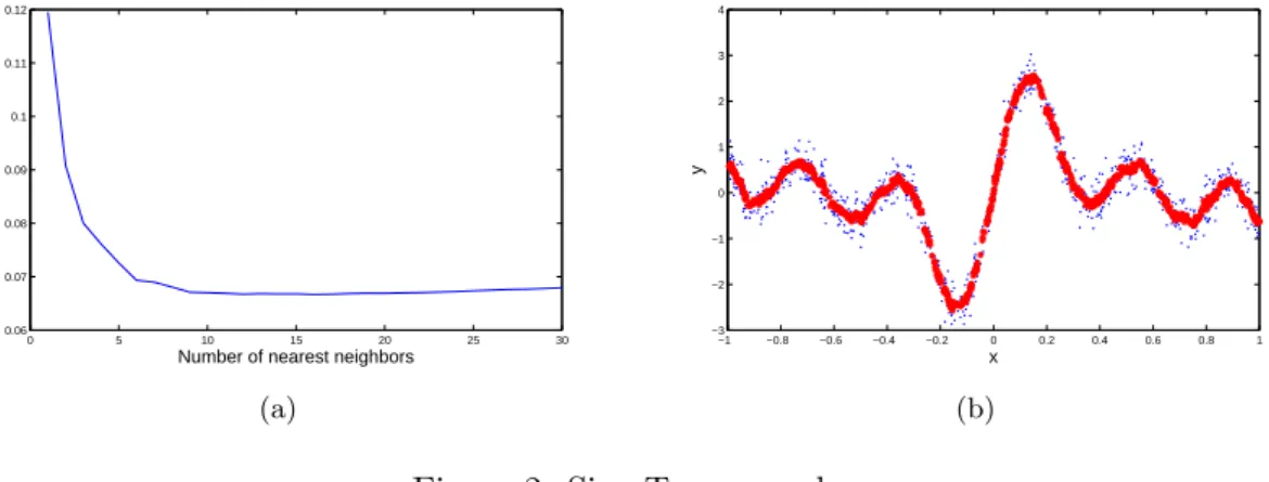
In this experiments, a set of 1000 training points are generated (and represented in Fig. 2B), the output is a sum of two sines. This single dimension example is used to test the method without the need for variable selection beforehand. The Fig. 2A shows the LOO error for different number of nearest neighbors and the model built with OP-KNN using the original dataset. This model approximates the dataset accurately, using 18 nearest neighbors; and it reaches a LOO error close to the noise introduced in the dataset which is 0.0625. The computational time for the whole OP-KNN is one second (using Matlab c implementation).
3.2 Financial Modeling
In this experiment, we use the data [11] related to 200 French companies during a period of 5 years. 35 input variables are used, these input variables are financial indicators that are measured every year (for example debt, number of employees, amount of dividends, . . . ). The target variables are
• The ROA defined as the ratio between the net income and the total assets. • The ROE represents the ratio between the net income and the capital.
0 5 10 15 20 25 30 0.06 0.07 0.08 0.09 0.1 0.11 0.12
Number of nearest neighbors
LOO Error (a) −1 −0.8 −0.6 −0.4 −0.2 0 0.2 0.4 0.6 0.8 1 −3 −2 −1 0 1 2 3 4 x y (b)
Figure 2: Sine Toy example
• The Marris (or Q ration) is calculated by dividing the market value of shares by the book value of shares
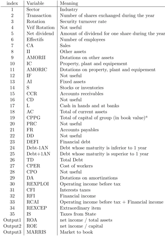
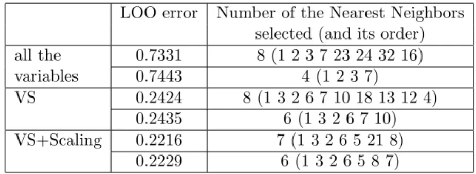
Table 1 shows the real meaning in financial field about all the variables we have used. All these three targets are tested one by one using OP-KNN; Variable Selection and Variable Selection+Scaling are performed beforehand [11] for comparison. The results are listed in the following Tables 2, 3 and 4 where we can see the LOO error are decreased almost half with variable selection step for each cases. The minimum LOO error appears when using OP-KNN on the scaled selected input variables as expected. Moreover, the final LOO error reach roughly the same stage as the value we estimated while doing variable selection [9]. Thus, for this financial dataset, this methodology not only build the model in a simple and fast way, but also prove the accuracy of our previous selection algorithm [9, 11]. It should be noted that on the example of this financial data, the integration of OP-KNN and Variable Selection phase shows the best efficiency and accuracy, meanwhile it selected the most important variables and build the model with them. The computational time for the whole OP-KNN is one second for each output.
4
Conclusions
In this paper, we proposed a methodology OP-KNN based on Extreme Learning Machine which gives better performance than the OP-ELM or any other algorithms for the financial modeling we have tested. Using KNN as a kernel, the MRSR algorithm and the PRESS statistic are all required for this method to build an accurate model. Besides, to do the prestep Variable Selection is clearly a wise choice to raise the interpretability of variables and increase the efficiency of the built model.
We test our methodology on 200 French industrial firms listed on Paris Bourse (Euronext nowadays) within a period of 4 years (1991-1995). Our results highlight that the first ten variables are the best combination to explain corporate performance. Afterward, the new variables do not allow improving the explanation of corporate performance. For example, we show that the company size is a variable that improves performance. Furthermore, it is interesting to notice that the discipline of market allows to put pressure on firms to improve corporate performance.
MASHS 2008, Creteil
Table 1: The meaning of variables index Variable Meaning
1 Sector Industry
2 Transaction Number of shares exchanged during the year 3 Rotation Security turnover rate
4 Vrif Rotation Not useful
5 Net dividend Amount of dividend for one share during the year 6 Effectifs Number of employees
7 CA Sales
8 II Other assets
9 AMORII Dotations on other assets 10 IC Property, plant and equipement
11 AMORIC Dotations on property, plant and equipement
12 IF Not useful
13 AI Fixed assets
14 S Stocks or inventories 15 CCR Accounts receivables
16 CD Not useful
17 L Cash in hands and at banks 18 AC Total of current assets
19 CPPG Total of capital of group (in book value)a
20 PRC Not useful
21 FR Accounts payables
22 DD Not useful
23 DEFI Financial debt
24 Debt-1AN Debt whose maturity is inferior to 1 year 25 Debt+1AN Debt whose maturity is superior to 1 year
26 TD Total Debt
27 CPER Cost of workers 28 CPO Not useful
29 DA Dotations on amortizations 30 REXPLOI Operating income before tax 31 CFI Interests taxes
32 RFI Financial income
33 RCAI Operating income before tax + Financial income 34 REXCEP Extraordinary item
35 IS Taxes from State
Output1 ROA net income / total assets Output2 ROE net income / capital Output3 MARRIS Market to book
a
Table 2: Normalized result for output 1
LOO error Number of the Nearest Neighbors selected (and its order) all the 0.7331 8 (1 2 3 7 23 24 32 16) variables 0.7443 4 (1 2 3 7) VS 0.2424 8 (1 3 2 6 7 10 18 13 12 4) 0.2435 6 (1 3 2 6 7 10) VS+Scaling 0.2216 7 (1 3 2 6 5 21 8) 0.2229 6 (1 3 2 6 5 8 7)
Table 3: Normalized Result for output 2
LOO error Number of the Nearest Neighbors selected (and its order) all the 0.9250 3 (1 8 2) variables 0.9246 2 (1 2) 0.9230 3 (1 2 5) VS 0.5437 5 (1 7 3 10 2) 0.5525 2 (1 2) VS+Scaling 0.5142 4 (2 1 4 8) 0.4951 11 (2 1 4 48 11 12 23 36 9 45 42)
Table 4: Normalized Result for output 3
LOO error Number of the Nearest Neighbors selected (and its order)
all the 0.9990 1 (63) variables 0.9942 2 (2 1) VS 0.7559 4 (1 4 13 15) 0.7594 2 (1 4) VS+Scaling 0.7058 6 (1 20 4 28 38 32) 0.7068 3 (1 20 4) 0.7088 2 (1 4)
MASHS 2008, Creteil
References
[1] G.-B. Huang, Q.-Y. Zhu, C.-K. Siew (2006), Extreme learning machine: Theory and applications, Neurocomputing, p. 489-501.
[2] B. Efron, T. Hastie, I. Johnstone, R. Tibshirani (2004), Least angle regression, Annals of Statistics, vol. 32 p. 407-499.
[3] R.H. Myers, (1990), Classical and Modern Regression with Applications, Duxbury, Pacific Grove, CA, USA
[4] G. Bontempi, M. Birattari, H. Bersini (1998), Recursive lazy learning for modeling and control, European Conference on Machine learning, p. 292-303.
[5] W.T. Miller, F.H. Glanz, L.G. Kraft (1990), Cmas: An associative neural network al-ternative to backpropagation, Proceeding of the IEEE, vol. 7097-102 p. 1561-1567. [6] C.R. Rao, S.K. Mitra (1972), Generalized Inverse of Matrices and its Applications, John
Wiley & Sons Inc,
[7] T. Simil¨a, J. Tikka (2005), Multiresponse sparse regression with application to multidi-mensional scaling, Proceedings of the 15th International Conference on Artificial Neural Networks, Part II p. 97-102.
[8] Y. Miche, P. Bas, C. Jutten, O. Simula, A. Lendasse (2008), A methodology for building regression models using Extreme Learning Machine: OP-ELM, European Symposium on Artificial Neural Networks, p. 23-25.
[9] Q. Yu, E. S´everin, A. Lendasse (2007), Feature Selection Methodology for Financial Modeling, Computational Methods for Modeling and Learning in Social and Human Sci-ence, Brest, France.
[10] A. Lendasse, V. Wertz, M. Verleysen (2003), Model Selection with Cross-Validations and Bootstraps - Application to Time Series Prediction with RBFN Models, Joint In-ternational Conference on Artificial Neural Networks, Istanbul, Turkey.
[11] Q. Yu, E. S´everin, A. Lendasse (2007), Variable Selection for Financial Modeling, Com-puting in Economics and Finance, Montr´eal, Canada.