HAL Id: halshs-00655585
https://halshs.archives-ouvertes.fr/halshs-00655585
Preprint submitted on 31 Dec 2011
HAL is a multi-disciplinary open access archive for the deposit and dissemination of sci-entific research documents, whether they are pub-lished or not. The documents may come from teaching and research institutions in France or abroad, or from public or private research centers.
L’archive ouverte pluridisciplinaire HAL, est destinée au dépôt et à la diffusion de documents scientifiques de niveau recherche, publiés ou non, émanant des établissements d’enseignement et de recherche français ou étrangers, des laboratoires publics ou privés.
Competing marital contracts? The marriage after civil
union in France
Marion Leturcq
To cite this version:
Marion Leturcq. Competing marital contracts? The marriage after civil union in France. 2011. �halshs-00655585�
Competing marital contracts?
The marriage after civil union in France
Marion Leturcq (PSE and CREST) ∗
June 2011† Preliminary
Abstract
Large changes in marital trends during the second half of the 20th
century raise the question of the reason leading to marriage in Western Europe and in Northern America: declining marriage rates, increase in cohabitation, increasing divorce rates. But the reason to get married can be diverse and can evolve over the life cycle. This paper examines is there is a demand for different marital contracts. In France, since 1999, two types of marital contracts are available: the marriage and the civil union (pacs). This paper investigates the substitution between the two contracts, by analyzing the distribution of the age at first marriage by cohort. It detects some recent changes in the bottom of the distribution of the age at first marriage, indicating a small impact of pacs on marriage. Therefore, it tends to conclude that substitution effects are likely to be very small and that the pacs reveals a demand for different marital contracts.
Keywords: civil union, marriage, substitution, quantile regression JEL Classification: J12, C21
∗Paris School of Economics, 48 boulevard Jourdan, 75014 Paris, France and CREST, Laboratoire de Microé-conométrie, 15 boulevard Gabriel Péri, 92245 Malakoff Cedex
1
Introduction
Societies in Western Europe and Northern America witnessed large changes in the household formation during the second half of the 20thcentury: less marriages, decrease in crude marital rates, but also in hazard rates, increasing divorce rates, cohabitation preceding marriage, and rising age at marriage. These changes denote a change in the demand for marital contracts, that can be linked to economic changes (education and labor supply of women) and to social norms (decrease in the stigma associated to divorce). But the supply of marital contracts has also evolved: most countries have passed less stringent divorce law, such as no-fault divorce, or unilateral divorce in the US. In many Western Europe countries, the supply for marital contract has also been extended: the claim of same-sex couples led to the creation of alternative marriage contracts, often called Civil Unions or Registered Partnership. In most countries, however, this alternative contract is available for same-sex couples only. But other countries, such as France, the Netherlands and Belgium, made it available to different-sex couples, creating a median way between cohabitation and marriage. The terms of Civil Unions contracts are very different from one country to the other, but a common feature is that they are easier to break up than marriage.
In France, the pacs1 has been created in 1999. While political debates mostly focused on giving a legal marital status to same sex couples, it has been opened to different sex couples since its creation. It is close to marriage, but easier to break up. The number of contracted pacs has been increasing since 2000. In 2009, two pacs are contracted for three marriages. Despite its success, little is known on the pacs: the lack of micro data makes it difficult to know who are the pacsed partners, why they contract a pacs and the link between pacs and marriage. Is there any substitution between the two contracts? Or are they considered as different contracts by couples?
The question of substitution between the two marital contracts address the issue of the use of marital contracts: is there a demand for different marital contracts? The economic theory of marriage examines the utility of marriage respect to cohabitation, considering that the main difference between the two contracts is that marriage is more costly to break up. The literature takes the opportunity of the adoption of unilateral divorce to evaluate the impact of lowering the costs of separation on marriage rates and investment in couple specific goods. The French case is even more interesting as it is not a type of contracts that replace another one, but the creation of two distinct contracts, implying horizontal differentiation in marital contracts. As a consequence, it proposes an original framework to evaluate what changing marital institutions indicates on marital behavior of couples. Substitution
1
pacs stands for Pacte Civil de Solidarité (Civil Pact of Solidarity). The word is now very common in French and some derivative have been rapidly created: the verb "se pacser" (that I will translate in "to pacs" means "to contract a pacs" and can be adapted in "to be pacsed", for example) is now in the dictionnary Le Larousse.
between pacs and marriage means that a contract facing lower costs of divorce is preferred. But if the substitution is dynamic: it would mean that the demand for marital contracts changes over time. This paper analyses the evolution of the marriage after the pacs is created. The goal of the paper is to evaluate if some substitution between pacs and marriage can be detected. In that purpose, I try to detect any change in the timing of marriage. I start with a period analysis that give how marriage evolves after the creation of the pacs compared to the period before. Then, I show that the timing of marriage can be summed up in the cumulative distribution function (CDF) of the age at first marriage for each cohort. So I try to detect changes in features of the CDF. I do not pay attention to classical features of the distribution such as mean and variance but to quantiles of the distribution. I try to detect if the quantile function conditional on cohort is changing after the creation of the pacs.
The paper shows that if any, the impact of pacs on the timing of marriage is rather small. Quite surprisingly, the pacs does not seem to affect much the timing of marriage.
After presenting the main evolution of marriage and pacs in France in section 2, I make explicit what could be the linked between pacsed and marriage in section 3. I analyse the evolution of marriage and of the mean age at marriage in section 4, and proposed an evaluation of the introduction of the pacs on quantiles of the distribution of the age at marriage in section 5. Section 6 concludes.
2
Marriage and pacs
2.1 Marriage: key historical changes
The second half of the 20th century witnesses large changes in the marriage law in France. It modified the relationship between the spouses and the link between children and marital status of their parents. The law evolved toward more equality between spouses. Since 1965, women can have a bank account and get a job without their husband consent. Equality between spouses is enacted in 1970: the father authority disappeared as the only authority in the household, it is replaced by parental authority. The divorce law changed to facilitate the exit from marriage. The no-fault divorce is made possible in 1975, but unilateral divorce is not permitted in France. Divorce procedure have been simplified in 2005 when spouses agree on the division of assets.
In the same time, the notion of parenthood has been progressively removed from the marital status. Since 1972, the law stipulates that acknowledged out-of-wedlock children have to be treated equal to in-the-wedlock children in terms of inheritance. As a consequence, the marriage of the parents of an out-of-wedlock child does not change anything in the eyes of the law. This equality has been extended to acknowledged children born of adultery in 2001, that are now equal in all respects to in-the-wedlock children. All differences between children according to the marital status of parents have been removed. Vital statistics on marriage do not register if he spouses already have children when they get married since 2005.
The consequence of these changes is that the marriage become a contract enacting the couple but not the family links, that are now independent of the marital status of the parents2.
The evolution of the law came jointly with the evolution of the household formation: the number of marriages is declining since the early 1970s (see fig. 1), while the number of out-of-wedlock births increased progressively. The number of out-of-wedlock births is greater than in-the-wedlock births since 2006. Most unions start with a cohabitation period: Toulemon (1996) indicates that in 1994, almost 90% of marriages started with a cohabitation period. As a consequence, the pacs has been created whereas the society experienced large changes in the household formation and marriage is not necessarily a stepping stone in the family formation.
2.2 The introduction of pacs: a competing contract?
The pacs was created in November 1999. It concludes 10 years of debates on the possibility to create a marital contract for same sex couples, as Denmark did in 1989. But it mostly concludes two years
2
The only remaining difference is that the father of a new born child is by default the husband when the mother is married, but the child has to be explicitly acknowledged by the father if the mother is not married.
of highly tense debates. The leading idea of the pacs was to provide a legal status to unmarried couples, therefore including same sex couples. However, the political debates mostly focused on the social consequences of providing same sex couples a legal form of union, that would entitle same sex couples to legal recognition.
At the beginning, the pacs has been made on purpose different from marriage (see tab. 1 for a comparison of the contracts). Pacs and marriage are similar to a certain extent: both contracts target couples: although the possibility to make the pacs available for relatives has been considered, it has not been left in the final text. Both ensure protection to partners: in case of death, the surviving partner can not be booted out the common housing. The pacs is a contract made to help partner "organizing their common life"3. As a consequence, pacsed partners are jointly responsible for debts and the pacs ensured by default a joint property of assets, unless the contract has been modified when it was signed. But the pacs was not created equal to marriage. Indeed, all couples can contract a pacs, including same sex couples. Moreover, a pacs can be break up with mutual consent or unilaterally. In those cases, a simple letter is enough to break up the union. A pacs is automatically broken up if at least one partner get married or in case of death of one partner. Even if the divorce procedure has been facilitated since 2005, it still requires at least an hearing with a judge (instead of two before 2005). Some institutional features distinguish the pacs from a marriage: it is a private contract and not a public institution as marriage. So it is privately contracted at the court, and not publicly at the town hall. The pacs is not considered as a stepping stone in the formation of a family: so it does not entitle couples for joint adoption nor survival benefit in case of death. It does not open the possibility to ask for citizenship. In case of death, a pacsed partner is not necessarily the heir of the deceased partner: a testament is needed and inheritance were taxed differently. While married couples could join their income for income taxation since the date of marriage, pacsed couples had to wait for three years before filling jointly one tax returns.
The pacs has been modified over time. In 2004, the interdiction to collect data on pacsed persons was raised, denoting that the pacs got more recognized as more and more couples, including different sex couples opt for the pacs. In 2005, the three years delay for joint income taxation of pacsed couples was suppressed. Leturcq (2011b) shows that it encouraged couples to contract a pacs. The largest change occurred in 2006: the law was modified to clarify the right and duties of pacsed partners. It also included a shift from joint to separate property of assets by default. In 2007, the taxation on inheritance between married spouses or pacsed partners were modified and made similar (but a testament is still required to designate the partner as the heir). So today, the main differences between
3
Loi nř99-944 du 15 novembre 1999, Art. 515-1 "Un pacte civil de solidarité est un contrat conclu par deux personnes physiques majeures, de sexe différent ou de même sexe, pour organiser leur vie commune."
the pacs and the marriage are the cost of separation, the possibility to adopt a child jointly, the lack of survivor benefit, the right to citizenship, and the pacs is still contracted in a court. Moreover, since 2007, the pacs is mentioned on birth certificates.
As denoted byFesty (2001), it was difficult to assess the pacs during its first years. It seemed to be more popular than in the Netherlands, but the lack of data made it difficult to understand the reason of that relative success. But the number of pacs contracted kept increasing both for same sex couples and different sex couples (Carrasco,2007). As the rate of increase is larger for different sex couples, the proportion of the same couples among pacsed couples decrease over time. 5% of pacsed couples are same-sex couples in 2009, the proportion was 25% in 2000. Micro data on pacsed couples are still not available. However, the analysis of data of a matched data set of tax returns and labour force survey (Enquête revenus fiscaux ) indicates that pacsed couples are more educated, have less children than married patners (Davie,2011).
To conclude, the distinction between marriage and cohabitation has been lowered over time. The pacs was created as an intermediary contract between cohabitation and marriage. But it has been modified and it is now closer to marriage. But it is still a different contract, especially because of lower costs of separation, which are considered in the economic literature as the corner stone of the difference between cohabitation and marriage. It raises the question of the horizontal differentiation of contracts and the substitutability of the two marital contracts.
The transition from pacs to marriage could not be studied using the data on dissolution of pacs provided by the Ministry of Justice because transition from pacs to marriage were not observed before 2007.4
4
When contracting a marriage, the pacs is automatically dissolved. So partners did not have to mentioned to the court that they were not pacsed anymore after a marriage. Until 2007, vital statistics (birth certificate) were not matched with data on pacsed partners. As a consequence, the dissolution following the marriage of one partner is unknown for the Ministry of Justice. In 2007, vital statistics were matched to birth certificate mentioning marriage and the data set on pacs dissolution has been updated: but all broken pacsed because of a marriage were attributed to 2007. As a consequence, the transition from pacs to marriage is not observed, and won’t be observed until some survey reconstruct the marital life of partners.
3
Links between marriage and pacs
3.1 Related literature: the economics of marital contracts
The economic literature on marriage has long ignored marital contracts. Since the seminal work by Becker, the literature has focused on couples: the theory of marriage is either a theory of matching (Becker, 1973, 1974) or a theory of household formation (Becker, 1981). But the development of cohabitation and the increase in divorce rates raised new issues: for example, link between marital instability and length of pre-marital cohabitation (Brien, Lillard, and Stern, 2006; Reinhold,2010), the cause of increasing divorce rate (impact of divorce laws: Wolfers(2006);Friedberg(1998)) and the consequences on investment in capital specific goods, such as children (Stevenson,2007;Drewianka,
2008).
The literature considers that couples can choose among two possibilities: cohabitation and mar-riage. Marriage is consider as a more committing relationship because it is more costly to dis-solve. Some studies have considered marriage and cohabitation in a static framework. They are based on the theory of cooperative game and they insist on marriage as a commitment device (Matouschek and Rasul,2008;Cigno,2009). The idea is that marriage induces cooperation by increas-ing the cost of separation. Therefore, low quality couples use marriage in order to foster cooperation. This idea concludes that marriage is used by low quality couples to enforce commitment.
But the link between marriage and cohabitation is complicated by dynamic. Static models fail to explain the development of cohabitation preceding marriage. Nowadays, a period of cohabitation tends to precede marriage (Stevenson and Wolfers,2007). InBrien, Lillard, and Stern(2006) cohabi-tation is explained by incomplete information about the quality of the match. Before marring, couples try to find out how good the match is. Therefore, it is a necessary step in the household formation as partners discover new information about the quality of the match in a repeated game. The authors link the length of the cohabitation duration to marital instability: the longer the cohabitation period, the less clear the match quality is and the higher the probability of divorce after marriage. The underlying idea is that imperfect information justifies the two step dynamic of the formation of the household. This idea echoes the seminal work by Mead (1970) proposing a two step marriage, i.e. a marriage that includes a first step as a trial for the couple.
In the model presented above, the marriage strengthens commitment between couples. But as marriage is considered as a long term partnership between two spouses, it highlights the willingness of the two partners to live together. As so, it can be considered as a signal toward to rest of the world (Bishop, 1984; Rowthorn, 2002; Leturcq, 2011a). But it can also signal to the other spouse
one’s willingness to form a household (Matouschek and Rasul,2008).
The models consider only two types of marital arrangement: cohabitation and marriage. However, the supply of marital contracts changed during the period in many countries. The claim for legal recognition by same sex couples led to the creation of different marital contracts. In many European countries, civil unions were created, although most of them are same-sex couples only. But some countries made civil unions available to both different sex and same sex couples (France, Netherlands and Belgium). They are marital contracts, more of less different from marriage (an interested reader should refer to Waaldijk (2005)). A key common feature of civil unions is that there are easier to break up than marriage, including the possibility of unilateral break up. In France, unilateral divorce is not permitted but a pacs can be unilaterally broken up. As such, the shift between pacs and marriage could be compared to the shift from no fault divorce to unilateral divorce in the US. However, in countries where civil union is made available to different sex couples, the new contract does not replace the old one, and it comes in addition to the marriage contract. Therefore, it provides a diversification in the supply of marital contracts.
Excluded Drewianka (2004), the literature has not studied the impact of the diversification of marital contracts on marital behavior. The understanding of potential links between marriage and pacs can be inspired by the literature on cohabitation and marriage. It can be understood as a less committing contract than marriage as it is less costly to dissolve, or as a different signal. But introducing a new type of marital contract has an ambiguous impact on the quality of the signal. Providing a kind of signal could improve the signalling of the couple, because it increases the supply of signals. But the quality of a signal depends on a universal agreement on the meaning of the contract. As it is a new contract, pacs can shape different meanings for pacsed couples (Rault,2009).
As a consequence, the analysis of the use of marriage, pacs and cohabitation requires first to understand better the substitutability between pacs and marriage. This could make clearer how close the marital contracts are in the use of partners. At time t, for a couple: pacs can substitute to marriage or to cohabitation. But the dynamic could be more complex: pacs could be a long term substitute to marriage, keeping couples away from marriage and inducing foregone marriages, or it could be a short term substitute inducing a delay in marriage.
3.2 Theoretical approach
3.2.1 The potential links between marriage and pacs
The following analysis investigates the potential links between pacs and marriage, by comparing what could be the behavior of couples if the pacs exists compared to how they would have behaved, the pacs has not existed. I assume that the creation of pacs does not affect the couple formation, so that the number of couples is the same as what it would have been without the pacs.
If the pacs does not exist, couples can only cohabitate or be married. The creation of the pacs adds a third possibility in the couples’ choices. As a consequence, at time t, it substitutes for cohabitation or for marriage. If it is a perfect substitute to marriage, the number of marriage is lower than what it would have been, but the number of unions is equal to what would have been the number of marriages. If it it is a perfect substitute to cohabitation: the number of marriage is not affected, and the number of legal unions is greater than what it would have been without pacs. The intermediate case would be that it is an unperfect substitute to both and the number of marriage is lower, but the number of unions is greater than the counterfactual number of marriages. If the counterfactual was observed, ie the number of marriage contracted at time t if the pacs has not been created, the substitution between pacs and marriage would be easily checked out. The observation of the joint evolution of the number of unions and marriage in fig. 2suggest that the pacs is an unperfect substitute to marriage, because the total number of unions increases while the number of marriages decreases. But, the counterfactual number of marriages is not observed, so it is unable to give the underlying link between pacs and marriage.
The substitution between pacs and marriage indicates if they are close contracts for couples. The utility derives from marriage is heterogenous in the population because of different demographic features (such as children) or different match quality. If pacs is a substitute for marriage then it affects those couples deriving better level of utility from marriage than cohabiting couples. If it is a substitute to cohabitation it affects those deriving from marriage lower level of utility. As a consequence, substitution to marriage indicates a low horizontal differentiation between contracts.
Utility derived from marriage can change over the life cycle (change in income, professional mo-bility, children, imperfect information on the match quality as in Brien, Lillard, and Stern (2006)): attitudes toward marriage and pacs can also changed over the life cycle. As a consequence, the links between pacs and marriage have to be considered in a dynamic framework.
If the pacs does not exist, there are only two types of couples: only cohabiting couples (type 1 couples) or couples cohabiting first (even if the cohabitation period is very short) and getting married
after a while (type 2 couples). But if the pacs is made available, four dynamics can be considered: only cohabiting couples; cohabitation and then pacs; cohabitation, pacs and marriage or cohabitation followed by marriage. The link between marriage and pacs depends on which type of couples alter their behavior. If pacsed couples would have been only cohabiting couples (type 1), the impact of pacs on marriage is very limited. It modifies the number of marriage contracted if couples, once pacsed, turn their mind toward marriage. Direct transition from cohabitation to marriage without pacs for type 1 couples are unlikely as it would violate the independence toward irrelevant alternatives assumption. On the contrary, if pacsed couples would have been type 2 couples, the links between marriage and pacs are more complex. A couple would have experienced a cohabitation spell before getting married can be affected by the pacs. If the new dynamic becomes cohabitation and then pacs, then the pacs can be considered as a long term substitute to marriage, inducing foregone marriage. The number of marriages is lower than what it would have been without the pacs, but the total num-ber of unions is the same as the numnum-ber of would-be marriages. The dynamic could also include a pacs spell between the cohabitation spell and the marriage spell. If the pacs replaces the cohabitation spell, without affecting the marriage date, then the pacs can be considered as a short term substitute to cohabitation and it has no effect on marriage. On the contrary, if it affects the marriage spell, the pacs induces a delay in marriage, with couples postponing their marriage. So it does not decrease the number of marriages over the life cycle, but it increases the number of unions contracted during the life cycle and it changes marriage rates over the life cycle.
The different scenarii proposed above show that the observation of marital behavior indicates how pacs and marriage are close substitute of not. Long term substitution to marriage indicates that there is no horizontal differentiation between contracts and they are competing marital contracts. On the contrary, short term substitution suggests that the utility derives from marital contracts evolves over time and pacs and marriage are competing for some part of the life. The lack of substitution points out that the horizontal differentiation between contracts is important.
From the discussion above, the substitution between pacs and marriage can be analyzed by a measure of the age an individual get married (the tempo component) and a measure indicating if individual eventually marry or not (the quantum component). Both indicators are features of the cumulative distribution of the age at marriage.
3.2.2 Period and cohort approach of tempo and quantum components
An important stream in the demographic literature attempts to disentangle in the observed decreas-ing marriage rate what comes from an increasdecreas-ing proportion of the population remaindecreas-ing unmar-ried their entire life and what comes from a part of population postponing marriage to older age (Goldstein and Kenney,2001). The quantum of marriage describes the number of ever married indi-viduals and the tempo describes the age the marriage is contracted. The main issue in this stream of the demographic literature is: how many times an individual is going to experience a certain event (here: marriage) in her life? The cohort-based approach consists in observing the cohort during its entire life-cycle and counting the number of unmarried individuals to characterize the quantum of marriage. The problem is that this approach prevents from analyzing recent trends in marital be-havior. The period-based approach is more popular as it permits the analysis of recent trends. The quantum is measured by the total marriage rate.5 It is merely defined as the proportion of marriages
that would be observed in a fictitious cohort experiencing at all ages the age marriage rates observed during the period. The problem is that this indicator is biased if individuals postpone their marriage. A bunch of papers attempt to extend the adjustment proposed byBongaarts and Feeney(1998). The adjustment is based on the observed evolution of the tempo of marriage, measured by the evolution of the mean age at marriage.
The two approaches answer different questions: the quantum of marriage for a given cohort is measured at the end of the life and describes the life of a cohort, that experienced different periods, while the period approach measures the quantum for a fictitious cohort and has to be read as an indicator of the social environnement at a given period.
The measure of the impact of pacs on marriage decisions is prone to another problem: the observed period is still a transition period. Three periods can be distinguished. Before the introduction of pacs, no cohort is affected by pacs. So the evolution of the number of marriage is explained by changes in the age structure of population and changes in the rates of marriage at different ages. During the transition period, the pacs is introduced at time t, so it affects different cohorts at different ages. Therefore, some cohorts are affected although part of the cohort is already married. Only the unmarried couples from this cohort are affected. But cohorts are not affected at the same age, meaning that the part of the cohort which is affected is different for each cohort. If there is some substitution between marriage and pacs, the introduction of pacs modifies the composition of unmarried couples at age a for a cohort attaining the age of a after the pacs is created compare to a cohort attaining the
5
The total marriage rate is an adaptation to marriage of the total event rates, which is the mostly used for the analysis of fertility.
same age before the pacs is created. After the transition period, all cohorts experienced the choice between pacs, cohabitation and marriage at all ages of their marital life. The 2000-2009 period is clearly a transition period, as the marital life cycle varies according to the definition between 18 and 50 or 18 and 60. As a consequence, the transition period challenges the quantum analysis. Indeed, period-based indicators relies on the extrapolation of old cohorts behavior on young cohort behavior, assuming that tempo changes are independent on cohorts. This statement can not be assessed since changes can follow the introduction of pacs. The change of the composition of the population also challenges the interpretation of period-based indicators of the tempo of marriage such as the mean age at marriage.
A cohort based approach seems more relevant. But, neither a cohort-based indicator of the quantum nor the mean age at marriage can be measured during the transition period, as the end of the marital life cycle is not observed for cohorts that started their marital life cycle after the introduction of pacs.
However, the cohort based analysis of the tempo of marriage is made possible using quantiles, as they feature the distribution of the age at marriage. The lowest quantile of the distribution of the age at first marriage are defined for recent cohorts. As a consequence, tempo changes can be detected if the quantiles of the distribution of the age at marriage changes across cohorts.
4
Period analysis: marriage trends
4.1 Data
Data on marriages come from Vital Statistics. It provides information on all marriages registered in France since 1965: birth date of the spouses, marriage date, and some personal information such as matrimonial status. Data on population come from the census. Census data are collected almost every 7 years in France (1968, 1975, 1982, 1990, 1999, 2006)6. Census provide information of people
according to the marital status, the age, the sex and diploma.
These data are the best to reconstruct cohorts, because they allow for the reconstruction of precise outflows of singles in the marriage at all ages, contrary to survey data. Therefore, they provide precise information on the quantiles of the distribution of the age at marriage.
The reconstruction of the outflows into marriage by cohorts requires some assumptions. Indeed, people face competing risks: they can die or move abroad before getting married in which case the marriage is not observed, and foreigners can move in France. Their marriage is observed if they marry in France but not otherwise. In order to construct the hazard rate of marriage, I need the at-risk of marriage population, i.e. singles. The survival of singles for a cohort is reconstructed across time by removing married individuals to the stock of singles observed at the beginning of the period thanks to census data. The difference between the reconstruction of remaining singles and the number of singles observed in the next wave of the census is explained by movers and deaths. I drop the difference uniformly from the number of singles reconstructed for each year between two waves of census.
Moreover, the marriage can be a repeated event over the life cycle. If the risk of remarriage increases, the distribution of the age at marriage can not be compared across cohorts. This is easily removed by considering only first marriages. The age at marriage is the age attained in the year.
4.2 The long run evolution of marriage
The long run evolution of marriage presented in fig. 1shows that marital trends change dramatically before the creation of pacs in 2000. The number of marriages increased in the late 60s before decreasing in the 1970s until the mid 1980s. It is still decreasing since then but at a lower rate. The number of marriages contracted per year is decreasing since 2000. However, the total number of unions outnumbers the marriages. In 2009, the total number of unions is close to the highest level of marriages in 1968. As a consequence, it seems rather impossible that the pacs is a perfect substitute
6
Since 2004, census is made continuously: 8% of the population is listed each year. 2006 stands for listed people between 2004 and 2009. Therefore, half the population is observed. The total numbers are imputed at the national level.
to marriage as the observed pattern of unions would have required a large increase in the marriage rates.
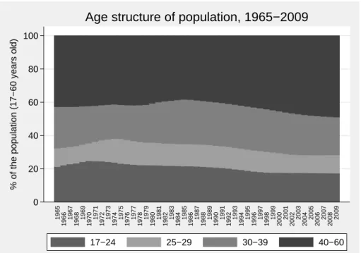
The level of the number of marriages can be explained by marriage rates and by the age structure of population. The structure by age of the population has changed over time (see fig. 3), and it could change the number of marriages as the marriage rates are not constant over ages. In order to detect if the changes are mostly explained by rates or population, I propose to decompose the evolution of marriages in a part explained by the evolution of the population compared to a reference date t0 and a part resulting in the change in the marriage rates:
M (t) − M (t0) = X a Rt(a)Pt(a) − X a Rt0(a)Pt0(a) = X a
[Rt(a) − Rt0(a)]Pt(a) +
X
a
Rt(a)[Pt(a) − Pt0(a)]
where M (t) is the number of marriage at date t, Rt(a) the rate of marriage at age a at date t, Pt(a) the population aged a at date t. The decomposition presented in fig.4shows that the evolution of marriages mostly comes from the evolution of rates, although the number of marriages would have been lower if the population has not kept increasing over the period. During the mid 1990s, baby boomers leave the age of high marriage rates, inducing a decline in the evolution of marriages. After 2000, the decline in the number of contracted marriages is explained by marriage rates.
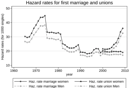
The hazard rates of marriage, defined as the number of marriage for 1000 individuals in fig. 5
give a rather different picture. After the large decrease in the 1970s and in the 1980s, it becomes very stable. The probability of contracting a union when single increases a lot after the introduction of the pacs, while the probability to contract a marriage when single is stable.
4.3 Period indicators: Marriage rates and mean age
Total marriage rate The total marriage rate a year t gives the proportion of married people of a fictitious cohort at the end of the life, if it has at each age the marriage rate observed for this age during the year t7. Although it is often considered as a measure of the quantum of marriage, it is not adapted to measure the quantum of marriage in transition periods, as it tends to underestimate the quantum for real cohorts if couples delay their marriage. As a consequence, the decrease of the
7 It is given by T M Rt= X a Mt(a) Pt(a)
unadjusted TMR is the result of the decrease in the number of marriage and the increase in the delay of marriage. Fig.6 shows that it tends to decrease dramatically until the late 1980s and remain stable after. Partial TMR at specific ages can be computed. Instead of integrated over the life cycle, partial TMR are computed on a certain age range. The sum of partial TMR is equal to the TMR. Partial TMRs give a better insight of the evolution of marriage. The partial TMR are given in fig. 7. The large decline of the TMR in 1965-1986 is explained by the large decline of marriage before 24 for women and men, but also by the decline of marriage rates between 24-29 for men. Although the TMR seems stable after 1986, the stability is explained by a two-fold dynamic. Between 1986 and 2000, the marriage rates of women aged 24-39 and men aged 30-39 increased, compensating the decline of marriage rates of youths. After 2000, the marriage rates of women aged 24-29 starts declining, while it keeps declining for men aged 24-29 years old, but the slope is steeper. The marriage rates at 30-39 stop increasing and become stable after 2000. Marriage rates after 40 years old keep increasing and is not negligible for men, although it is very low for women. As a consequence, the two main changes after 2000 are affecting 25-39 years old individuals.
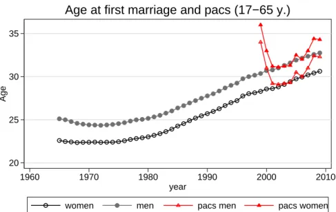
The age at first marriage: why does it increase? The mean age at first marriage increased gradually since 1971 (fig8). It can not be directly read as the sign that the couples delay their marriage because it is driven by two forces: the age structure of the population and the marriage rates at each age. It can be decomposed into the part explained by the population and the part explained by rates. Denoting Pt(a) the population aged a at t, Rt(a) the marriage rate of the population aged a at t (Rt(a) = Mt(a)/Pt(a)), Pt=PaPt(a) the total population at t and Rtthe marriage rate at t (at all ages, Rt= Mt/Pt), then the mean age can be written as:
Xt= X a Pt(a) Pt | {z } =nt(a) Rt(a) Rt | {z } =rt(a) a
As a consequence, the evolution of the mean age at first marriage can be written as:
Xt− Xt0
| {z }
∆X
= X
a
nt0(a)(rt(a) − rt0(a))a
| {z }
Sr
+X
a
(nt(a) − nt0(a))rt(a)a
| {z }
Sn
The left part (Sr) of the equation gives how would have evolved the mean age at first marriage, if the population have stayed the same as in t0. The right part (Sn) indicates what is explained by
the evolution of the structure of the population. In the following, I group ages into 4 age groups.
Fig. 9decomposes the evolution of the age at first marriage in Sr and Sn. It shows that while the evolution of rates explains the shape of the evolution of the age at first marriage, the age structure of the population has compensated the decline in the age at first marriage that would have been more than 2 years lower for men in the early 70s. Since 1995, the mean age at first marriage would have increased more without the decline explained by the age structure of the population.
Fig. 10 decomposes the impact of rates and population on age at first marriage by age groups. The decrease in the age at first marriage before 1970 is explained by the increase of the number of young people less than 24. The increase in the age at first marriage due to changes in the age structure of population between 1970 and 1995 is mostly explained by the increase in the population aged 24-29 years old. It corresponds to the baby-boom cohorts. After 1980, the increase in the age of marriage is explained by the changes in the rates of marriage of older people aged 24-39 years old. The joint evolution of the number of 24-29 and 30-39 years old people and their marriage rates explains the increase in the age at first marriage.
There is no major disruption after 2000 in the evolution of the mean age at marriage. It is interesting to notice that the age of pacsed partners (different sex)8 are similar to the age at first marriage, and are evolving the same way between 2001 and 2006. Today, the age at pacs is even greater. It could be linked to what was observed on TMR: the partial TMRs of persons aged 25-39 tend to decrease are become stable, indicating that there might be some substitution between pacs and marriage at these ages.
8
Data of the age of pacsed partner come fromCarrasco(2007) for 1999-2006. 2007-2009 is reconstructed using data of the mean age of different sex pacsed partners provided by the ministry of justice under the assumption that the mean age difference between men and women is constant and equal to 2.
5
Delayed marriages? A cohort analysis
5.1 Detect delaying and foregone marriages: a quantile approach
As explained above, if the pacs affects the marriage decision, the pacs can be seen as either a long term substitute or a short term substitute to marriage.
If it is a long term substitute, it induces foregone marriages, meaning that part of the population is not going to get married during their life: the proportion of unmarried individuals at the end of their life time is greater than what it would have been the pacs has not been created. As it is measured at the end of the life (or at an high enough age to consider that it is very unlikely that the remaining unmarried part of the population is going to marry), it is defined at the cohort level.
If pacs is a short term substitute to marriage, it induces that some couples delay their marriage because they decide to pacs first. It means that compared to another cohort, the probability to get married is lower at some ages but it increases afterward. At the end of the life, the proportion of unmarried individuals is the same for both cohorts.
As a consequence, delaying and foregone marriages can be detected analyzing the cumulative distribution function (CDF) of age at marriage for a cohort compared to its counterfactual. As for duration models, the basic assumption is that everybody is getting married at the end, but some are getting married very late, so the marriage is not observed because data are censored (either because of death or because end of the period of observation). A foregone marriage can be seen as a censored duration or as a delayed marriage after the death. So it is difficult, if not impossible, to estimate the part of foregone marriage up to a certain age. Before this age, a foregone marriages is difficult to distinguish from a delayed marriage.
The analysis of delaying marriage is based on the definition of the quantile function, conditional on the cohort. Let’s consider two cohorts. The CDF of the age at marriage is F0 for the older cohort and F1 for the younger. The conditional quantile function defines delayed and foregone marriages:
1. Let’s define a foregone marriage an unmarried individual at age a. It means that Fk(a) = τk 6= 1. If there are more foregone marriages for the younger cohort, it is detected by τ1 < τ0. So, the existence of foregone marriages means that quantiles q(τ ) for τ greater than τkare not defined. However, this measure requires the observation of the cohort at least up to the age a.
2. Delayed marriages means that the younger cohorts marry later. Delaying at all ages means that F1 is stochastic dominated by F0. A pure delaying does not induce foregone marriages, so that F0(a) = F1(a) = τ . So all quantiles qk(τ ), for τ ≤ τ are defined for both cohorts, with q1(τ ) > q0(τ ).
3. If the delay is homogenous in the population, ie the delay for couples getting married young is the same as the delay for couples marrying late (q1(τ ) − q0(τ ) = δ, ∀τ ), then this could be express a a location shift of the CDF. But if the delay is heterogenous in the population (q1(τ ) − q0(τ ) = δ(τ )), affecting only early marriage for example, then it could also be linked to a scale shift of the CDF.
The effect of cohort on the quantile is the quantile treatment effect (QTE) and it is measured by the distance q1(τ ) − q0(τ ). As a consequence, an impact of pacs on the number of marriages and the timing of marriages could be detected with the evolution of quantiles by cohorts, as long as previous cohorts provide a good counterfactual to younger cohorts.
5.2 A cohort based approach
5.2.1 Reconstructing cohort
The analysis of the evolution of quantiles across cohorts requires the reconstruction of the cumulative distribution function of the age at marriage by cohort. A cohort is composed of all individuals born the same year, and the CDF gives how the cohort flow out to married status. As a consequence, I only consider the age at first marriage.
It is not possible to observe the age at first marriage for the whole cohort because individuals face competing risks: death and out-migration, that can occurs before marriage. As a consequence, the size of the observable at-risk population changes over time. Moreover, the size of the cohort is also modified by in-migration. In order to analyse the CDF of the age at first marriage, I need to fix the size of the cohort, contrary to the period analysis presented above. The following describes how I fix it.
The mis-specification of the cohort can leads to under/over estimate the flow in marriage. If the reference size is the size at the beginning of the marital life9, then those who die before being married are denoting as unmarried at the end of the life. So it would lead to overestimate the number of foregone marriages, especially if the probability of dying tend to be bigger for ages such as the older cohorts are already married but not the younger cohorts. More over, this is also a problem as it increases the quantile at a given τ . But if the reference size of the cohort is the last observation for the size of the cohort, because dying married individual are counted in flow in marriage but not in
9
The minimal age to get married without the consent of the parents is 18 years old in France for both men and women since 1974. However, between 1974 and 2006, women could get married if they were between 15 and 18 years old with the consent of parents. It has been increased to 18 for women in 2006. Before 1974, the minimal age to get married without the consent of the parents was 21 years old for both men and women (since 1907), but women could married with the consent of the parents if they were more than 15 years old and men if they were more than 18 years old.
the cohort size. This would tend to underestimate the size of the cohort, and it could lead to a CDF greater than 1, which is obviously not a desired property.
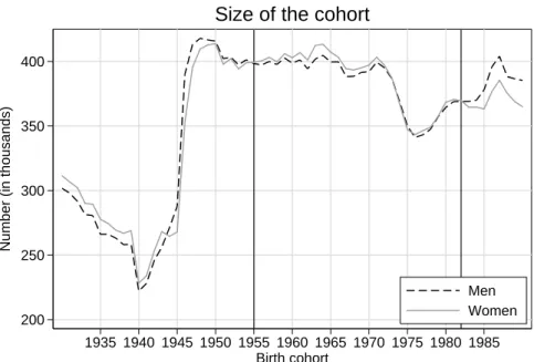
So I consider that the cohort is composed of singles at the end of the period I observe (age in 2009 or 60 years old) and individual getting married during the period I observe. As a consequence, singles dying before marriage are not counted in the cohort size. When I do not observe the beginning of the marital life (i.e. cohorts before 1950 for women and before 1947 for men) the cohort size is given by the number of singles at the end of the period, added to those getting married during the period and to those that are married at the beginning of the period I observe. So individuals dying before getting married during the period and individual already dead before the beginning of the period of observation (married of not) are not counted in the cohort size. As a consequence, the cohort size is given by a restrictive definition of cohort, including the risk of death. In other words, data on marriage are not censored, except by the end of the period of observation.
The in-migration flows increase the cohort size, making it difficult to define a cohort including mi-gration. As a consequence, I only consider the age at first marriage for French citizen. The citizenship is defined as the citizenship at the age of marriage, observed in the vital statistics. Naturalization could modify the size of the cohort. If naturalization occurs before marriage then the individuals is part of the cohort. The size of the reconstructed cohort is given in fig. 11.
The problem raised by migrations prevents from analyzing the evolution of cohorts at a more precise geographic scale because the cohort size is more variable.
For the precise determination of quantile, an individual is said to be married at age X if she was over this age (in month) when marrying.
5.2.2 The evolution of marriage by cohort
The evolution of marriage rates is described by the density function (type 1 rate), the cumulative function and the hazard function (type 2 rates).
The evolution of marriage rates by cohort can be divided into 5 periods. The evolution is similar for men and women, although I keep different cohorts as turning points for men and women to illustrate this evolution, as men tend to marry older than women. The main evolutions are presented on figures12 for men and 13 for women.
For the cohorts born before 1951 (for men) and 1954 (for women), the marriage rate by age is stable: the density and the cumulative function are almost the same. Men and women tend to marry young: the density reaches a maximum at 22 for men and 20 for women: more than 30% of the cohort is already married the year men turn 22 and women turn 20. At 25, 77% of women born in 1948
are married. At 28, 76% of men born in 1945 are married. However, the hazard rate starts declining after 23 for men and 20 for women, indicating that remaining singles tend to marry less.
The marriage rates at early ages (before 26 for men and 24 for women) decline sharply for cohorts born in 1951-1962 and 1954-1963 for women. It increases for older ages, but not enough to compensate the decline: 17% of women born in 1963 are married at 20 years old, and 48% of them are married at 25 years old and 70% at 35, while 89% of the 1948 cohort was already married at 35. 15% of men born in 1961 are married at 22, 48% are married at 28 years old and 64% at 35, it was 85% of the cohort born in 1945. This decline is linked to a large decrease in the hazard rate up to 32 for men and 28 for women. The hazard rate does not get greater for younger cohorts at older ages. It means that remaining singles never tend to increase their marriage rate compared to older cohorts. Despite the large decrease, the marriage rates remain the highest at 19-20 years old for women, 22-23 for men.
The following period witnesses a shift in the marriage rates by age. While marriage rates keep declining before 26 for men and 24 for women, they keep increasing after, inducing a shift in the age the marriage rate is the highest. For men born in 1968, the marriage rate is the highest at 26 and for women born in 1971, the marriage rate is the highest at 25 years old. However, the increase at older ages does not compensate the decrease at younger ages: 58% of women born in 1971 are married the year they turn 35, 53% of men born in 1968 are married at 35. The hazard rate keeps declining until 29 for men and 26 for women. Then it remains stable across periods: the hazard rate of marriage for younger cohort never exceed the hazard rate for older cohort, whatever the age.
The marriage rates for women born between 1971 and 1975 are stable, while the marriage rate for men born in 1968-1976 keeps decreasing and shifting: the marriage rate is the highest at 27-28. The marriage rates starts decreasing again for women born after 1975 and men born after 1976. 6% of men and 14% of women born in 1983 are married at 25.
In addition to the shift in the mean age at marriage, the variance of the rates of marriage has increased a lot. For cohorts born in the 1940’s, the sharpness of the density of marriage rates traduces the weight of social norms around marital habits. The decline of marriage rates has also diluted the age considered as normal to get married.
To conclude, two main evolutions has to be taken into account: the transition starts with an increase in the variance of the age at first marriage. It is followed by a shift in the mean age at first marriage. The variance keeps increasing for recent cohorts. The following analysis attempts to see if there is a link between the recent evolution of cohorts and the creation of the pacs.
5.3 Empirical strategy
5.3.1 Defining the treatment
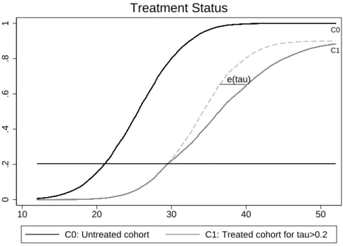
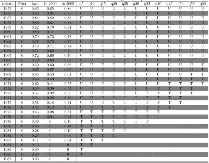
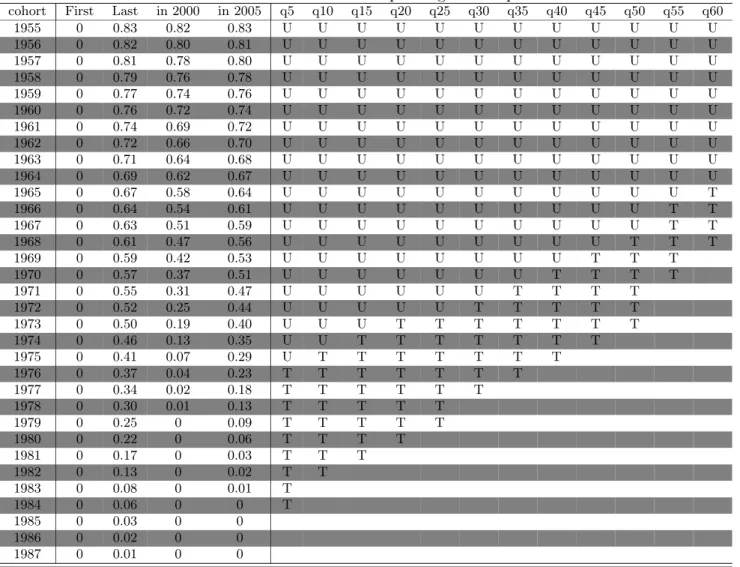
Estimating the impact of pacs on marriage requires the definition of treated units. The intuitive definition considers that an individual is treated if she is not married when the pacs is created. Thus, for a given cohort, some individuals are treated and some are not, depending if they are married when the pacs is created. Therefore, if the pacs is created when τ *100% of the population is treated, the determination of the first quantiles up to q(τ ) are not affected by the pacs, because they are determined before the pacs is created. But higher quantiles are likely to be affected by the creation of the pacs. Therefore, a cohort is considered untreated for the first quantiles of the distribution up to q(τ ) and treated for quantiles larger than q(τ ). Denoting C the cohort and t the date of the creation of the pacs, FC(t − Ci) gives the number of married individual among the cohort C at the age t − C, when the pacs is created. So the treatment status is given by
Ti(τ ) = 1{FC(t − Ci) < τ } (1)
Fig. 14 illustrates the definition of the treatment status. As a consequence, a cohort can be untreated for the determination of a quantile but treated for the determination of another quantile. Treated and untreated cohorts for different quantiles are detailed in table 3 for men and table 2 for women.
Notice that the composition of the unmarried population at a rank τ depends on when the cohort starts being treated. Indeed, let’s consider two cohorts: the pacs is created when the cohort C0 attains the rank in the distribution τ0 and when the cohort C1 attains the rank in the distribution τ1 with τ1 < τ0 (the cohort 1 is younger). So, if there is some substitution between pacs and marriage, the composition of the unmarried population is different when the two cohorts attain the rank τ , because some individuals in cohort C0 got married between the age q(τ1) and q(τ0) but they would not have been married if the pacs has existed at that time. It means that the treatment effect at a given quantile is not likely to be constant across cohorts, because it affects different populations.
5.3.2 A quantile regression approach: identification issues
A before-after estimation on quantiles
Qai(τ |Ci) = α(τ ) + δCi(τ ) + ηCi(τ )Ti(τ ) (2)
where ai is the age at first marriage, Ci is the cohort of individual i and Ti indicates if the cohort has been treated for this quantile as given in eq. 1, δCi(τ ) is the cohort effect for this quantile.
ηCi(τ ) is the quantile treatment effect at rank τ , for a cohort Ci. This framework does not give any
functional form for the effect of the cohort on the quantile and for the effect of the treatment on the quantile. However, this framework meets the standard identification problem that a cohort can not be observed both treated and untreated for a quantile, preventing the identification of δCi(τ ) and
ηCi(τ ) 10.
A simple difference identifies ηCi(τ ) if δCi(τ ) is constant across cohorts. But δCi(τ ) = δ(τ ), ∀Ci
imposes some stability on the repartition of the ages at first marriages because it imposes that the age such as τ ∗ 100% of the cohort is already married is constant across cohorts. It seems to be a strong assumption, except for cohorts born during the 1940’s.
A standard difference in difference identifies the impact of treatment under restrictive assumptions. Consider 3 cohorts, C = 0, C = 1 and C = 2. Only the last cohort, C = 2 is treated at rank τ . The difference in difference on quantiles identifies (with a simplified writing):
[Q(τ |C = 2) − Q(τ |C = 1)] − [Q(τ |C = 1) − Q(τ |C = 0)] = [δC=2(τ ) + ηC=2(τ ) − δC=1(τ )] − [δC=1(τ ) − δC=0(τ )] = ηC=2(τ ) if [δC=2(τ ) − δC=1(τ )] = [δC=1(τ ) − δC=0(τ )]
The identifying assumption [δC=2(τ ) − δC=1(τ )] = [δC=1(τ ) − δC=0(τ )] is true if δC(τ ) = δ(τ ) ∗ C ie if the evolution of the quantile follows a linear trend. This assumption is strong as it assumes that the evolution of the quantile between C = 1 and C = 0 describes well the evolution between C = 2 and C = 1. It does not allow non linear evolution of quantiles such as a period of stability of the age at marriage following a shift. Under this assumption, the estimator is a simple before-after estimator, figure15 sums up the identification of the quantile treatment effect in that case.
Despite its simplicity, the analysis of non parametric quantiles in figure 17for men and figure19
for women shows that the linear trend assumption is not a bad approximation for cohort born after 1960 for low (τ ∈ [5, 25]) and medium (τ ∈ [30, 50]) quantiles, and for cohort born after 1955 for
10
The CQF can be written using the classic Rubin framework: Qai(τ |C) = Q (1) ai(τ |Ci)Ti+ Q (0) ai(τ |Ci)(1 − Ti) with Q(0)ai(τ |Ci) = α(τ ) + δCi(τ )and Q (1) ai(τ |Ci) = α(τ ) + δCi(τ ) + ηCi(τ )
higher quantiles (τ ∈ [55, 75]).
Notice that the quantile treatment effect ηCi(τ ) is not necessarily constant across cohorts. An
important problem is that if there is substitution between pacs and marriage, the introduction of pacs changes the composition of the unmarried population at a given age. So, the longer the period between the introduction of pacs and the age the cohort attains when τ ∗ 100% is married is, the more affected the cohort is. I take this possibility into account including a trend for treated units.
The estimated equation is
Qai(τ |Ci) = α(τ ) + δ(τ )Ci+ [η0(τ ) + η1(τ )Ci]Ti(τ ) ≡ z
′
iβ(τ ) (3)
where Ti is a dummy indicating if the individual belongs to a treated cohort and Ci is a contin-uous variable for the cohort. The vector of parameters β(τ ) is estimated using quantile regressions.
Koenker and Bassett (1978) have showed that β(τ ) can be estimated by minimizing in β: 1 n n X k=1 ρτ(ai− z′β)
where ai is the age at first marriage for individual i and ρτ(u) is the objective function such as:
ρτ(u) = τ × u, for u ≥ 0 (1 − τ ) × u, for u < 0
The variance of the conditional quantile Qai(τ |Ci) is given by V (qτ) =
τ(1−τ )
f2(qτ) where f is the
density of the outcome (at). The estimation of the variance requires the non parametric estimation of the density function f . In order to avoid such estimation, the standard errors of the coefficients are estimated by bootstrap.
The CQF is censored as the quantile is not necessarily defined for youngest cohorts. The last de-fined quantile for each cohort is indicated in table 3for men and2 for women. I estimate the impact of treatment on uncensored quantiles, so the composition of cohorts used for the estimation changes depending on the quantile. An estimation including censored quantiles would be a nice extension.
Any change in the trend of the CQF after the pacs is created is going to be interpreted as a treatment effect. But it could also be explained by a break in the trend if a change is occurring at the same time of the introduction of pacs. So it is difficult to have a causal interpretation of the results, because causality stems from the trend assumption which is a stringent assumption.
Moreover, the quantile treatment effect (QTE) is not identified if cohort fixed effect are integrated in the model. But interquantile regressions can provide an estimation of the QTE when cohort fixed effects are included.
A DiD model using interquantile distances
Let’s consider the most general model for the conditional quantile function, as given by the eq. 2:
Qai(τ |Ci) = α(τ ) + δCi(τ ) + ηCi(τ )Ti(τ )
The evolution of the CQF could be due to some cohort fixed effects across quantiles. It could be included in the cohort effect, written as a part depending on τ and a fixed part:
δCi(τ ) = γCi(τ ) + µCi
The before-after estimation presented above does not identify the treatment effect ηCi(τ ) if cohort
fixed effects are included, even if the impact of cohort on quantile is linear with γCi(τ ) = γ(τ )Ci.
Indeed:
[Q(τ |C = 2) − Q(τ |C = 1)] − [Q(τ |C = 1) − Q(τ |C = 0)] = [γ(τ ) ∗ 2 + µ2+ ηC=2(τ ) − γ(τ ) − µ1] − [γ(τ ) + µ1− µ0] = ηC=2(τ ) + [µ2− 2µ1+ µ0]
Including cohort fixed effects is important if some large changes are affecting all individuals of a cohort and modifying their behavior towards marriage, in a sense which is not taken into account by the linearity of the CQF in the cohort. Such changes could be a rise in education attainment, a change in the minimal required age to get married. However, a cohort fixed effect affect equally all quantiles, inducing a location shift of the conditional cumulative distribution function. Most large changes are not likely to affect all quantiles the same way, but could affect part of the distribution. The identification strategy presented below is based on pair wise comparison of quantiles, so it enables to drop cohort fixed effects that are common to the two quantiles and thus allowing for fixed effect for part of the distribution. If cohort fixed effects are assumed to affect locally the distribution, a comparison of close quantiles is suffisant to drop the cohort fixed effects.
quantiles defined at τ0 and τ1, with τ1> τ0. The interquantile distance is given by:
Qai(τ1|Ci) − Qai(τ0|Ci) = [α(τ1) + γCi(τ1) + µCi+ ηCi(τ1)Ti(τ1)]
−[α(τ0) + γCi(τ0) + µCi + ηCi(τ0)Ti(τ0)]
= [α(τ1) − α(τ0)] + [γCi(τ1) − γCi(τ0)] + [ηCi(τ1)Ti(τ1) − ηCi(τ0)Ti(τ0)]
In the following, let’s define ∆Ci(τ0, τ1) = Qai(τ1|Ci) − Qai(τ0|Ci) Let’s assume that there are two
cohorts, C = 1 and C = 2. The former is not treated for τ0 and τ1, but the latter is treated for τ1 but not for τ0. As a consequence:
∆C=2(τ0, τ1) − ∆C=1(τ0, τ1) = [γC=2(τ1) − γC=2(τ0)] − [γC=1(τ1) − γC=1(τ0)] + ηC=2(τ1)
Therefore, ηC=2(τ1) is identified if [γC=2(τ1)−γC=2(τ0)] = [γC=1(τ1)−γC=1(τ0)]. So it is identified if γC(τ ) is constant across cohorts, which is a strong assumption. But it is not identified under an assumption of linearity such as γCi(τ ) = γ(τ ) ∗ Ci. Because in that case:
∆C=2(τ0, τ1) − ∆C=1(τ0, τ1) = γ(τ1) − γ(τ0) + ηC=1(τ1)
As a consequence, ηC=2(τ1) is identified by difference in difference in difference, considering a third cohort C = 0 which is not treated both at τ1 and at τ0. It comes:
[∆C=2(τ0, τ1) − ∆C=1(τ0, τ1)] − [∆C=1(τ0, τ1) − ∆C=0(τ0, τ1)] = [γ(τ1) − γ(τ0) + ηC=1(τ1)] − [γ(τ1) − γ(τ0)]
= ηC=1(τ1)
This method requires untreated cohorts and cohorts only treated for τ1.
Comparing the treated cohort at τ1 (C = 2) to a cohort C = 3 which is treated both at τ0 and τ1 gives an estimation of:
In that case, comparing to a third cohort which is not treated both in τ1 and τ0 leads to the identification of ηC=2(τ1) − ηC=3(τ1) + ηC=3(τ0) but neither the QTE at τ0, ηC=3(τ0) nor the QTEs at τ1.
If the QTE at τ1 is assumed to be linear in the cohort: ηC(τ ) = η0(τ ) + η1(τ )C, ηC=2(τ1) − ηC=3(τ1) = η1(τ1), which is identified by the comparison of untreated cohorts to a cohort treated only in τ1.
As a consequence, under the assumption that the QTE is linear and considering a continuum of cohorts such that T (τ0) and T (τ1) are not always equal, the QTE is identified in the model:
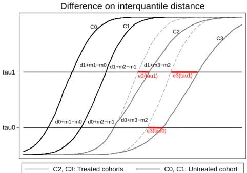
∆Ci(τ0, τ1) = a(τ0, τ1) + d(τ0, τ1)Ci+ [η0(τ1) + η1(τ1)Ci]Ti(τ1) + [η0(τ0) + η1(τ0)Ci]Ti(τ0) (4)
As for the difference in difference estimation, the trend in the QTE takes into account the evolution of the composition of the unmarried population. The schema 16 illustrates the identification.
The identification relies heavily on the assumption of continuity: the pacs was not created, the interquantile distance d(τ0, τ1) would have evolved the same way.
T (τ0) is not necessarily equal to T (τ1). Of course, T (τ0) implies T (τ1) because if the cohort is treated for a low quantile, it is also treated for a higher quantile. But the contrary is not necessarily true, especially because the pacs was created at a given period, affecting all cohorts at different ages. However, if the compared quantiles are very close, T (τ0) ≈ T (τ1) challenging the estimation.
The estimation of the interquantile distance requires the joint estimation of two quantiles. The variance of the estimator requires the estimation of the variance of the estimator for each quantiles and the covariance. Therefore, the variance is estimated by bootstrap.
5.4 Results
5.4.1 Evolution of quantiles
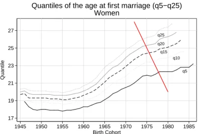
The evolution of quantiles is given by fig. 19 and 20 for women and fig. 17 and 18 for men. The evolution is similar for both men and women. All quantiles are stable for the cohorts born in the 1950s. The last quantiles (higher than q40) increase for older cohorts born in the 1950s, while the lower quantiles remain stable. Lower quantiles start increasing for cohorts born in the 1960s. It tends to show that social changes do not affect all the population at the same. While part of the population keeps marrying with the same pattern, another part of the population changes its marital behavior. The overall evolution of quantiles denotes the increasing delay of the first marriage as all quantiles
increased across cohorts. This delay can be observed at all ranks of the distribution: even the lowest quantile increased with cohort. But the quantiles also denote the increasing variance in the age of marriage, meaning that the social norms around marriage are diluting. Highest quantiles increase sharply with cohorts, denoting the increasing number of foregone marriages.
No disruption in the evolution of quantile can be observed after the creation of the pacs, except that lower quantiles tend to increase at a lower rate.
The interquantile distance compares the evolution of quantiles τ1 to a baseline quantile τ0. It means that it compares, for a given cohort, the marital behavior of the population getting married early to those getting married older. An increasing distance between quantiles indicates the behavior toward marriage is not changing at the same rate for different population. Interquantile distances are presented in fig. 22 for women and in fig. 21 for men. I take as baseline quantiles Q5, Q10 and Q20. The labels T1 (resp. T0) indicates that the higher τ1 (resp. lower τ0) compared quantile was defined after the creation of pacs. What ever the baseline quantile, the interquantile distance increases over time, especially for cohorts born after 1960. The slope is larger for higher quantiles, denoting the increasing variance of the age at first marriage across cohorts. The distance between Q5 and Q10 is very stable across cohorts. As a consequence, the interquantile distance of other quantiles to Q10 is very similar to the distance to Q5. Although any clear change can not be detected after the introduction of pacs for men, the interquantile distance between highest quantiles and Q10 or Q20 is increasing at a higher rate after the introduction of pacs for women.
5.4.2 Before-After model: quantile regressions
I propose different specifications to estimate eq.3. The first one only includes a constant and a trend for cohort. The second introduces a dummy for the treatment of the creation of the pacs as defined in eq.1 and a trend for cohort after the creation of pacs, to take into account the change in the composition of the unmarried population. I also test an alternative definition of the treatment, that defines as treated a cohort for which the quantile was defined after 2005 and not 2000. This is to take into account the spread of information on the pacs across cohorts and the large increase in the number of pacs contracted after 2005 because of the reform of income taxation of pacsed couples. I then run the same estimation by adding a quadratic trend on cohorts. The same specifications are run on two set of cohorts: the first one only includes cohorts born after 1960, the second one adds 1955-1960 cohorts. The impact of the creation of pacs is evaluated at 12 ranks of the distribution of the age at marriage, for every five percentiles between Q5 and Q60. I only show results for Q5, Q20
and Q50, for the first set of cohorts. Indeed, as indicated above, the increase started for cohorts born after 1960 for lowest quantiles. Complete results are available in a separate appendix.
The treatment status of cohorts depends on the studied quantile: table3 for men and table 2for women give the treatment status for each cohort depending on the quantile. Tables 4 to 9 gives the results of the quantile regressions. The coefficient on cohort is stable across specifications. Adding a quadratic trend seems relevant as it is significant in many specifications. The treatment status is significant for lower quantiles but not for higher quantiles. Surprisingly, the treatment status is negative for lower quantile, meaning that under the assumption of constant trend across cohort, the treatment tend to lower the age at marriage for those getting married early. This effect seems surprising as it is unexpected. However, the total impact of the treatment has to be computed in order to discuss the impact of the creation of the pacs. The second definition of treatment is not significant. As a consequence, any changes in the timing of marriage have to be detected before 2005. My favorite specification includes a trend and a quadratic trend in cohort, a dummy for treatment in 2000 and a trend for treated cohorts (column (6))
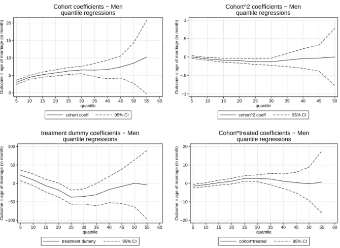
The coefficients of the quantile regressions are plotted in figure 24 for men and figure 23 for women. Not surprisingly, the coefficients on cohort are increasing over quantiles, meaning higher quantiles tend to vary more with cohort than lower quantiles. The quadratic trend is significant for intermediate quantiles, although it is slightly significant for men. The coefficients on treatment show interesting pattern. The dummy for treated cohort positive and significant, while the trend for cohort after the treatment is negative for lower quantiles. The intermediate quantiles, the signs are the contrary.
The total impact of treatment for a given cohort can be reconstructed at each rank of the distri-bution with:
ˆ
η(τ ) = ˆη1(τ ) ∗ cohort + ˆη0(τ )
Fig. 27for women and28for men reconstruct the impact of treatment for two cohorts. The cohort of females born in 1975 is affected after the 20th percentile. The impact of pacs is not significant on the distribution of the age at marriage. However, the cohort born in 1977 is affected since the 10th percentile. Lowest quantiles are negatively affected: the age such as 10% of the 1977 cohort is married is 5 months lower than what it would have been without pacs. This result can be interpreted as a sign that the youngest cohort are affected negatively by the creation of pacs, meaning that they tend to marry younger than what they would have done the pacs was not created. It can also be interpreted as the sign that the identifying assumption is not likely to hold here, and that the lower quantiles
![[PDF] Débuter avec le logiciel Nikon Capture étape par étape | Cours informatique](data:image/gif;base64,R0lGODlhAQABAIAAAP///wAAACH5BAEAAAAALAAAAAABAAEAAAICRAEAOw==)