Shift in diversification in sister-clade comparisons: a more powerful test

HAL Id: hal-01822124

https://hal.archives-ouvertes.fr/hal-01822124

Submitted on 23 Jun 2018

HAL is a multi-disciplinary open access

archive for the deposit and dissemination of sci-entific research documents, whether they are

pub-L’archive ouverte pluridisciplinaire HAL, est destinée au dépôt et à la diffusion de documents scientifiques de niveau recherche, publiés ou non,

Shift in diversification in sister-clade comparisons: a

more powerful test

Emmanuel Paradis

To cite this version:

Emmanuel Paradis. Shift in diversification in sister-clade comparisons: a more powerful test. Evolu-tion - InternaEvolu-tional Journal of Organic EvoluEvolu-tion, Wiley, 2012, 66 (1), pp.288 - 295. �10.1111/j.1558-5646.2011.01429.x�. �hal-01822124�

Running head: SHIFT IN DIVERSIFICATION

SHIFT IN DIVERSIFICATION IN SISTER-CLADE

COMPARISONS: A MORE POWERFUL TEST

Emmanuel Paradis

Institut de Recherche pour le D ´eveloppement, ISEM UMR 226/5554 – UM2/CNRS/IRD, Jl. Taman Kemang 32B, Jakarta 12730, Indonesia

E-mail: Emmanuel.Paradis@ird.fr

Tests of shift in diversification associated with key innovations or directional environmental change can be performed with sister-clade comparisons. This approach is attractive because it does not require detailed phylogenetic

information. I propose a new likelihood ratio test based on fitting two models of diversification. I show how this test differs from a previous likelihood ratio test based on the geometric distribution. With simulations from a wide range of situations, I show that the new test performs much better than this test and the traditional test by Slowinski and Guyer. The proposed test performs at least as well as the species richness contrast test which has been proposed by several authors in four versions. A power analysis with low number of pairs of

sister-clades showed that the new test could detect a shift in diversification with five or less pairs of sister-clades, while the diversity contrast test cannot detect any shift in this situation. The former appears as more powerful than the latter, and therefore is recommended when the number of pairs of sister-clades is low (less than ten). All other tests should not be used as the present study showed they lack statistical power and robustness.

The factors driving evolutionary diversification can be classified into two categories: intrinsic to the species (e.g., morphological traits, physiological features, genetic structure and variability), and extrinsic to them (e.g., climatic variables, food resources, interspecific competition). Both categories of factors clearly interact because the adaptive value of a species trait is linked to a

particular set of environmental variables. In order to test the relative influence of these two categories of factors, we need to formulate predictions on the variation in diversification rates as can be observed in real data, either fossil or recent. Generally, we may expect intrinsic factors to result in variation among clades, whereas extrinsic factors result in temporal variation. Statistical methods have been developed to test these two classes of hypotheses. The problem of testing for temporal variation in diversification has been shown recently to be

particularly difficult (Stadler, 2009; Rabosky, 2010; Paradis, 2011). The problem comes mainly from the fact that different combinations of speciation and

extinction rates may result in very similar distributions of branching times, even when these two parameters are constant through time (Paradis, 2011).

On the other hand, the statistical methods testing for inter-clade variation in diversification rate do not seem to suffer from the same problem. Some

remarkable progress have been accomplished in the analysis of phylogenetic trees combined with discrete or continuous traits (Paradis, 2005; Maddison et al., 2007; FitzJohn et al., 2009; FitzJohn, 2010). Such sophisticated methods have been used by Goldberg et al. (2010) to investigate the evolutionary forces behind the maintenance of self-compatibility among species of Solanaceae.

In the absence of detailed fossil data, it seems very likely that methods based on phylogenies are the most informative. However, though phylogenetic and

molecular data are accumulating at high pace, detailed phylogenies are currently available only for a restricted number of groups. In this perspective, statistical methods based on the comparison of species richness between sister-clades appears as a valuable approach to test hypotheses on variation in diversification rate. The basic data structure to test such hypotheses is a series of sister-clades where one clade is characterized by a trait or an environment that is absent or different in the other. The aim is to test whether this trait or environment has increased diversification rate.

In this paper, I introduce a new statistical test for the analysis of this kind of data. This test is related to the one introduced by McConway and Sims (2004); however, using simulations I show that the former is more robust and more powerful. I also compare these two tests with the classical test by Slowinski and Guyer (1993) and the species diversity contrast.

Tests of Diversification Shift

Consider the data as n pairs of sister-clades: x1iand x2iare the species richnesses

for the ith pair, and the subscripts 1 and 2 are the two states of the variable under focus (trait, environment, or other). In the followings, and for the simplicity of the text, state 1 will be called key-innovation. Let us further denote as xi

(i = 1, . . . , 2n) the species richness of any clade in the data.

Slowinski and Guyer (1993) built a test based on calculating the probability of all possible data sets that are less compatible with the null hypothesis than the observed one. This probability is calculated for each pair of sister-clades. A combined probability testing the global null hypothesis (i.e., with all pairs) is

calculated with Fisher’s combined probabilities −2 ∑n_i ln pi: this follows a χ2

distribution with 2n degrees of freedom. The alternative hypothesis is that diversification rate is higher in clades characterized by the key-innovation. Thus the test is a one-tailed test and it cannot detect whether diversification rate is lower in those clades. Because of its design, the Slowinski–Guyer test is particularly prone to type I error in situation of U-shaped species richnesses (Goudet 1999; Vamosi and Vamosi 2005; see also the discussion below).

Barraclough et al. (1996) developed a species diversity contrast test which can be written as:

sign(x1i− x2i)ln max(x1i, x2i)

ln min(x1i, x2i), i = 1, . . . , n.

This contrast is computed for each pair resulting in n values on which nonparametric statistics are applied to test the null hypothesis. Vamosi and Vamosi (2005) pointed out that this test shares its rationale and general structure with three others: the one used by Wiegmann et al. (1993) who computed the logarithm of the ratio:

lnx1i

x2i = sign(x1i− x2i) ln

min(x1i, x2i)

max(x1i, x2i),

as well as the one by Barraclough et al. (1995) with:

sign(x1i− x2i)max(x1i, x2i)

x1i+ x2i ,

Vamosi and Vamosi (2005, p. 575) and Vamosi (2007) made a detailed comparison of these four variants of the species diversity contrast test, and recommended to use either of the two first ones with either a matched-pair randomization procedure if n ≤ 12, or a Wilcoxon test otherwise. Because all these tests can be written as sign(x1i− x2i) ×Ci, the randomization procedure is

easily done by randomizing only the signs (Ci= |x1i− x2i| for Sargent’s version).

The Barraclough et al.’s (1996) version has the logarithm of the smallest value between x1i and x2i, thus this can lead to a division by zero if it is equal to one. In

this situation, one needs to add one to all xi’s. In all the variants of the diversity

contrast test, the test may be one- or two-tailed.

McConway and Sims (2004) devised an alternative test based on the probability distribution of species numbers as given by a model of random speciation and extinction with rates λ and µ, respectively. Let us denote this number by X, and assume for simplicity that there is no extinction (µ = 0). Starting from a single species (X0= 1) the probability of Xt, the number of

species at time t, is given by Yule (1924, eq. 5):

Pr(Xt= x|λ) = e−λt(1 − e−λt)x−1, (1)

This, therefore, applies to stem group richness. The Appendix shows the same equation for µ > 0.

McConway and Sims set β = 1 − e−λt _{in order to draw an analogy between}

equation (1) and the geometric distribution whose probability density function is β(1 − β)x−1. They used a likelihood function optimized over β in the case of the null hypothesis, or over β1and β2for the alternative hypothesis. The likelihood

ratio is calculated for each pair of sister-clades. These ratios are then summed over the n pairs: this likelihood ratio test (LRT) follows a χ2distribution with n degrees of freedom. Like the diversity contrast tests, the McConway–Sims test can be one- or two-tailed.

I propose to optimize the likelihood function over λ using equation (1). In theory this requires to know the dates of origin t, but in practice this appears unimportant as these can be set equal to an arbitrarily large value (say 103_{; see}

simulation results below). This has an important consequence because if t is large then e−λt will tend to zero, and the transformation used by McConway and Sims (2004) will give β ≈ 1 even if λ varies. The other major difference with the McConway–Sims test is that the 2n clades are considered as independent

observations; thus a single LRT is computed. The likelihood function under the null hypothesis is:

2n

∏

Pr(Xt= xi|λ),

and under the alternative hypothesis:

n

∏

Pr(Xt = x1i|λ1) Pr(Xt= x2i|λ2).

The log-transformed likelihood functions are optimized over λ, and λ1and λ2,

respectively. The LRT is computed with twice the difference in the maximum log-likelihood: it follows a χ2distribution with one degree of freedom. The derivation of this test assumes that diversification rates and times of origin are homogeneous across sister pairs. The robustness of the test to situations where

these assumptions are not met is assessed in the next section.

Simulation Study

Methods

The present simulation study aimed at contrasting the statistical properties of the four tests. The scenarios were selected in order to characterize situations of varying statistical power (probability of rejecting the null hypothesis when it is false). Following McConway and Sims (2004), I first simulated data from a geometric distribution with parameters β1and β2(here and below, the subscript

of the parameter stand for the trait state). This repeats some of the simulations done by McConway and Sims (2004). I only considered two scenarios: one where the null hypothesis is true (β1= β2= 0.9), and one where it is false

(β1= 0.9, β2= 0.7).

The second set of simulations also repeats some from McConway and Sims (2004): this uses a negative binomial distribution, a situation they found to be less favorable to their test. The negative binomial distribution is a generalization of the geometric one with an additional parameter denoted as ν. I considered six scenarios with ν = 0.5, 0.9, or 1.2 combined with the two parameter sets from the previous paragraph.

The third set of simulations used a Poisson distribution with parameter γ1= 10 and γ2= 10, 15, or 20.

These three sets of simulations considered n = 35 like in McConway and Sims (2004), and were replicated 10,000 times.

In the fourth set of simulations, species numbers were taken from

phylogenies simulated from a speciation–extinction model with parameters λ1,

λ2, µ1and µ2. Five series of parameters were selected: (i) the null hypothesis is

true (λ1= λ2, µ1= µ2); (ii) the null hypothesis was false by moderately

increasing λ2; (iii) the value of λ2was the same than in the previous series but µ2

was also slightly increased; (iv) the increase in λ2was stronger; and (v) the same

than previously with an increased value of µ2. All phylogenies were simulated

starting 35 units of time before present. In order to test the robustness of the tests to the lack of homogeneity among lineages, two additional sets of simulations were run. In the fifth set, λ1was randomly drawn from a uniform distribution

whose interval width was 0.1 and mean equal to the value chosen in the previous set; λ2was then fixed with the same contrast than previously. Another set of

simulations where both λ1and λ2were random gave similar results which are

reported in the Supplementary Information. Finally, in the sixth set the time of origin of each phylogeny was randomly drawn from a uniform distribution in the interval [10, 50]. These last three sets were simulated with n = 10 or 20, and replicated 1000 times.

After running these six sets of simulations, the two most powerful tests were selected for a detailed estimation of their statistical power with very low n (1, . . . , 10). The data were simulated from a speciation–extinction model with the

following parameters: λ1= 0.1, λ2= 0.12, 0.14, . . . , 0.2, and µ1= µ2= 0.09.

In all sets, the rejection rate was calculated as the proportion of tests where the null hypothesis was rejected at the usual rate of 5%. The rejection rate is an estimate of the type I error rate when the null hypothesis is true, and an estimate of the power of the test when the alternative hypothesis is true. All simulations

and analyses were programmed in the R language (R Development Core Team, 2010) version 2.13.0, and function tests are available inape(Paradis et al., 2004). An annotated R script is available in the Supplementary Information showing how to perform these simulations, assess type I/II error rates as well as other analyses. A Sweave document (.Rnw) is also provided as an example of how to use this script to repeat the detailed power analysis with low n.

Results

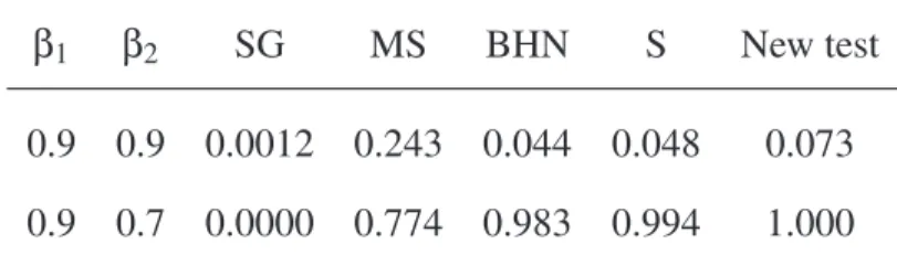
The four versions of the diversity contrast test gave close results. Somehow surprisingly, Sargent’s (2004) version performed the best among these four while Barraclough et al.’s (1996) performed the worst. The two other versions gave the same results which were intermediate. Therefore I report only the two first results here. Repeated simulation runs showed that the estimates of rejection rates were accurate to ±0.002. Thus, all proportions were rounded to the third digit. The detailed results are in the Supplementary Information.

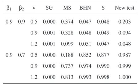
In all scenarios, the new test and the two versions of the diversity contrast test performed much better than the two others (Table 1–4). The only situation where the new test performed poorly was when data were simulated from a negative binomial distribution with ν = 0.5: the type I error rate reached 0.2 but the McConway–Sims test performed even worst (Table 2). On the other hand, the diversity contrast test kept its type I error rate close to 0.05. However, when the null hypothesis was false with the same negative binomial distribution, the new test appeared slightly more powerful than the diversity contrast test when ν = 0.5. The power of both tests was close to one with ν = 0.9 or 1.2.

With data simulated from a Poisson distribution, the diversity contrast test appeared as the most powerful one, though the new test had comparable power, and close to one, for the most contrasting situation with γ1= 10 and γ2= 20

(Table 3).

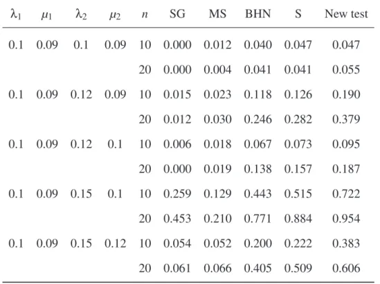
With data simulated from phylogenies, only the diversity contrast tests and the new one showed good properties, the latter having higher power (Table 4). The Slowinski–Guyer and McConway–Sims tests showed significant power only when the clades with the highest diversification had a low extinction rate

compared to the speciation rate, that is λ2= 0.15 and µ2= 0.1. When µ2was

increased to 0.12, the power of these two tests was lost even with n = 20 pairs while the power of the new test reached 0.6, and the power of the diversity contrasts test was 0.4 and 0.5 for Barraclough et al.’s and Sargent’s version, respectively (Table 4).

Heterogeneity among lineages did not affect the performance of the tests (Table 5). On the other hand, heterogeneity in the origin time of the lineages affected negatively the power of all tests but the new one (Table 6). For the new test, two versions were computed here: the first one assumed that the times of origin t were unknown and set to 1000, and the second one used the simulated values (results within parentheses in Table 6). Surprisinly, the first version had greater power, though its type I error rate was slightly inflated.

Overall, the Slowinski–Guyer test appeared to perform very poorly as it failed to reject the null hypothesis in all scenarios. Thus the type I error rate was kept at a low level, but the power of the test was low as well. The only situation where some significant power was observed was simulating phylogenies with a λ2= 0.15 and µ = 0.1 (Table 4). In this situation, this test was more powerful

than the McConway–Sims test but much less than the new test. The

McConway–Sims test showed variable performances: its power was good with data from a geometric or a negative binomial distribution; however, the type I error rate was quite high in these situations, reaching 0.38 with ν = 0.5. These results only partially replicate those from McConway and Sims’s (2004) simulation study which showed no sign of inflated type I error rate in similar situations. Considering that this test appeared as not to be recommended because of its poor performance in other situations, I did not explore this issue further.

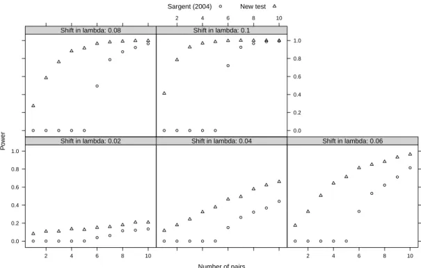
The detailed power analysis with low n therefore concerned Sargent’s version of the diversity contrast test and the new test (Fig. 1). The diversity contrast test cannot detect any shift in diversification when n < 6. On the other hand, the new test can detect a shift even when n = 1: the estimated power was 0.412 for

λ2= 0.2 with a single pair of clades, and was 0.986 with n = 5. The power of the

new test was greater than 0.6 when 3 ≤ n ≤ 5 for λ2≥ 0.16.

Discussion

Finding the factors promoting or preventing the diversification of evolving lineages is one of the current challenges for evolutionary biologists. At the interspecific level, this problem can be addressed with four types of data: fossil data, phylogenies of recent species, species richnesses combined with ages of stem/crown groups, and species richnesses of sister-clades. All other forms of data (e.g., raw species richnesses) have to be considered as inappropriate because they lack a temporal dimension. Among these four kinds of data, the last one must be considered the coarsest because the temporal dimension is only relative,

thus limiting the inference on relative contrast in diversification. Nevertheless, the approach is interesting precisely because it does not require accurate

phylogenetic information or molecular dating. Recent applications of sister-clade comparisons include a test of increased diversification among myrmechorous angiosperm clades (Lengyel et al., 2009), and a comparison of gall-inducing and non-galling insect lineages (Hardy and Cook, 2010).

Vamosi and Vamosi (2005) reviewed the properties of some tests of

sister-clade comparison: the Slowinski–Guyer test, the sign test, and the species diversity contrast test. They did not consider the McConway–Sims test in their study arguing that it is likely that this test shares some of the properties of the Slowinski–Guyer test. The simulation results presented in this paper confirm this suspicion since the rejection rates of these two tests varied somewhat in parallel. A surprising result was that the difference contrast test used by Sargent (2004) performed slightly better than the versions by Wiegmann et al. (1993) and

Barraclough et al. (1996). This may come from the fact that the simple difference makes less assumption on the distribution of the diversity contrasts compared to other versions.

The simulations with heterogeneous diversification parameters showed an interesting results: all tests were robust to this heterogeneity in the sense that the rejection rates were very close to those observed with homogeneous parameters. Overall, the new test presented here and the difference contrast test showed the most acceptable statistical properties. The advantage of the new test

compared to Sargent’s (2004) was a higher power when data were simulated from phylogenetic trees. On the other hand, the new test appeared to have an inflated type I error rate with data simulated from a negative binomial with a low

variance (ν = 0.5); however, the type II error rate was the lowest among the tests considered here with this distribution.

One should be cautious in concluding that the new test is generally more powerful than the others because the simulated scenarios are only a small fraction of the possible ones. Therefore we cannot exclude that in some cases, not considered here, this will not be the case. However, the R script provided with this paper may help to assess this issue by simulating other specific scenarios. The detailed power analysis showed that the new test works even in situations where the diversity contrast test collapses (i.e., n ≤ 5).

Vamosi and Vamosi (2005) examined in detail a problem encountered with the Slowinski–Guyer test: if species richnesses are U-shaped (highly skewed but in a symmetric manner with respect to the trait analyzed), then this test will find a significant effect of the trait on diversification. They illustrate this fact with the following data: x1= {216, 64, 33, 2, 3, 1} and x2= {3, 1, 2, 33, 216, 64}. The

Slowinski–Guyer test is significant: χ2

12= 22.63, P = 0.031. However, both

series of species richnesses are identical though differently ordered. The

explanation is that species richness differences contribute in an asymmetric way depending on their direction. For instance, the first pair (216, 3) contributes the

P-value p1= 0.014, while the fifth pair (3, 216) contributes p5= 0.991. After

logarithmic transformation (i.e., −2 ln pi), these contribute 8.572 and 0.018 to the

overall χ2_{. So the fifth pair contributes only to increasing the number of degrees}

of freedom. The McConway–Sims test is also significant: χ2

6= 28.277,

P < 0.001. The Sargent test does not suffer from this problem because it tests for

also avoids this difficulty because under the alternative hypothesis the maximum likelihood estimates will be the same (ˆλ1= ˆλ2). Therefore the likelihood values

under both hypotheses will also be equal, leading to χ2₁= 0.

In order to avoid the increased type I error rate related to Fisher’s method of combining probabilities, the Z-test may be used instead (Whitlock, 2005). However, this does not solve the problem of the very low power of the

Slowinski–Guyer test as was shown by a limited number of simulations (results not shown).

To conclude, previous studies have suggested to not use the Slowinski–Guyer test because of its lack of power (McConway and Sims, 2004) or high type I error rate (Vamosi and Vamosi, 2005). The present study largely agrees with these conclusions. Furthermore, it is shown here that the likelihood ratio test proposed by McConway and Sims (2004) is not robust because it lacks some statistical power when data do not follow a geometric distribution. I suggest to use either the difference contrast test used by Sargent (2004), or the new test proposed here. The former has an acceptable type I error rate in a wide range of situations, whereas the latter is more powerful and should be preferred when the number of pairs of sister-clades analyzed is low (n < 10) and is robust to heterogeneity in diversification rate among clades. Furthermore, the new test is the only

applicable with very low n (< 6) and can have substantial power in this situation.

Acknowledgments

I am grateful to Jana Vamosi and two anonymous reviewers for their constructive comments. I thank Bernard Hugueny for comments on an earlier version of the

manuscript. Financial support was provided by grant ANR-09-PEXT-008-01. This is publication IRD-DIVA-ISEM 2011-096.

LITERATURE CITED

Barraclough, T. G., P. H. Harvey, and S. Nee. 1995. Sexual selection and taxonomic diversity in passerine birds. Proc. R. Soc. Lond. B 259:211–215. Barraclough, T. G., P. H. Harvey, and S. Nee. 1996. Rate of rbcL gene sequence

evolution and species diversification in flowering plants (angiosperms). Proc. R. Soc. Lond. B 263:589–591.

FitzJohn, R. G. 2010. Quantitative traits and diversification. Syst. Biol. 59:619–633.

FitzJohn, R. G., W. P. Maddison, and S. P. Otto. 2009. Estimating

trait-dependent speciation and extinction rates from incompletely resolved phylogenies. Syst. Biol. 58:595–611.

Goldberg, E. E., J. R. Kohn, R. Lande, K. A. Robertson, S. A. Smith, and B. Igi´c. 2010. Species selection maintains self-incompatibility. Science 330:493–495. Goudet, J. 1999. An improved procedure for testing the effects of key

innovations on rate of speciation. Am. Nat. 153:549–555.

Hardy, N. B. and L. G. Cook. 2010. Gall-induction in insects: evolutionary dead-end or speciation driver? BMC Evol. Biol. 10:257.

Kendall, D. G. 1948. On the generalized “birth-and-death” process. Ann. Math. Stat. 19:1–15.

Lengyel, S., A. D. Gove, A. M. Latimer, J. D. Majer, and R. R. Dunn. 2009. Ants sow the seeds of global diversification in flowering plants. PLoS ONE

4:e5480.

Maddison, W. P., P. E. Midford, and S. P. Otto. 2007. Estimating a binary character’s effect on speciation and extinction. Syst. Biol. 56:701–710. McConway, K. J. and H. J. Sims. 2004. A likelihood-based method for testing

for nonstochastic variation of diversification rates in phylogenies. Evolution 58:12–23.

Paradis, E. 2005. Statistical analysis of diversification with species traits. Evolution 59:1–12.

Paradis, E. 2011. Time-dependent speciation and extinction from phylogenies: A least squares approach. Evolution 65:661–672.

Paradis, E., J. Claude, and K. Strimmer. 2004. APE: analyses of phylogenetics and evolution in R language. Bioinformatics 20:289–290.

R Development Core Team, 2010. R: A Language and Environment for Statistical Computing. R Foundation for Statistical Computing, Vienna, Austria. URL: http://www.R-project.org.

Rabosky, D. L. 2010. Extinction rates should not be estimated from molecular phylogenies. Evolution 64:1816–1824.

Sargent, R. D. 2004. Floral symmetry affects speciation rates in angiosperms. Proc. R. Soc. Lond. B 271:603–608.

Slowinski, J. B. and C. Guyer. 1993. Testing whether certain traits have caused amplified diversification: an improved method based on a model of random speciation and extinction. Am. Nat. 142:1019–1024.

Stadler, T. 2009. Lineages-through-time plots of neutral models for speciation. Math. Biosci. 216:163–171.

sister-group comparisons. An addendum. Evol. Ecol. Res. 9:717.

Vamosi, S. M. and J. C. Vamosi. 2005. Endless tests: guidelines for analysing non-nested sister-group comparisons. Evol. Ecol. Res. 7:567–579.

Whitlock, M. C. 2005. Combining probability from independent tests: the weighted Z-method is superior to Fisher’s approach. J. Evol. Biol. 18:1368–1373.

Wiegmann, B., C. Mitter, and B. Farrell. 1993. Diversification of carnivorous parasitic insects: extraordinary radiation or specialized dead end? Am. Nat. 142:737–754.

Yule, G. U. 1924. A mathematical theory of evolution, based on the conclusions of Dr. J. C. Willis, F.R.S. Phil. Trans. R. Soc. Lond. B 213:21–87.

Appendix

The probability for a lineage originated from a single species to have x species after a time t giving speciation and extinction probabilities λ and µ is (Kendall, 1948): Pr(Xt= x|λ, µ) = (1 − ζt)ζtx−1, where ζt =        λ(e(λ−µ)t− 1) λe(λ−µ)t_{− µ} if λ 6= µ, λt 1 + λt if λ = µ.

This probability is conditioned on the lineage surviving until present (Xt ≥ 1).

Setting µ = 0 leads to equation (1).

It does not appear straightforward to use these formulae to derive a test similar to the one introduced above because of the difficulty of the additional extinction parameter(s) leading to more complicated likelihood expressions. Furthermore, there are now a more complex set of hypotheses related to shifts in diversification. The null hypothesis of no shift in diversification may be false because of an increase in speciation rate, a decrease in extinction, or both.

Table1: Rejection rates of the null hypothesis for five tests when data were

simu-lated from a geometric distribution with parameters β1 and β2(35 pairs of sister-clades). SG: Slowinski and Guyer (1993), MS: McConway and Sims (2004), BHN: Barraclough et al. (1996), S: Sargent (2004).

β1 β2 SG MS BHN S New test

0.9 0.9 0.0012 0.243 0.044 0.048 0.073

Table2: Rejection rates of the null hypothesis for five tests when data were

sim-ulated from a negative binomial distribution with parameters β1, β2, and ν. The size (or shape) parameter ν was the same in both series (35 pairs of sister-clades). Abbreviations as in Table 1. β1 β2 ν SG MS BHN S New test 0.9 0.9 0.5 0.000 0.374 0.047 0.048 0.203 0.9 0.001 0.328 0.048 0.049 0.094 1.2 0.001 0.099 0.051 0.047 0.048 0.9 0.7 0.5 0.000 0.188 0.852 0.877 0.987 0.9 0.000 0.737 0.974 0.990 0.999 1.2 0.000 0.813 0.993 0.998 1.000

Table3: Rejection rates of the null hypothesis for five tests when data were

sim-ulated from a Poisson distribution with parameters γ1 and γ2 (35 pairs of sister-clades). Abbreviations as in Table 1.

γ1 γ2 SG MS BHN S New test

10 10 0.000 0.000 0.045 0.044 0.000

10 15 0.000 0.000 1.000 1.000 0.258

Table4: Rejection rates of the null hypothesis for five tests when data were

sim-ulated from a birth–death process with speciation rates λ1and λ2and extinction rates µ1and µ2. n: number of pairs of sister-clades. Abbreviations as in Table 1.

λ1 µ1 λ2 µ2 n SG MS BHN S New test 0.1 0.09 0.1 0.09 10 0.000 0.012 0.040 0.047 0.047 20 0.000 0.004 0.041 0.041 0.055 0.1 0.09 0.12 0.09 10 0.015 0.023 0.118 0.126 0.190 20 0.012 0.030 0.246 0.282 0.379 0.1 0.09 0.12 0.1 10 0.006 0.018 0.067 0.073 0.095 20 0.000 0.019 0.138 0.157 0.187 0.1 0.09 0.15 0.1 10 0.259 0.129 0.443 0.515 0.722 20 0.453 0.210 0.771 0.884 0.954 0.1 0.09 0.15 0.12 10 0.054 0.052 0.200 0.222 0.383 20 0.061 0.066 0.405 0.509 0.606

Table5: Same than in Table 4 except that λ1was randomly drawn from a uniform distribution

U

in the interval [0.05, 0.15] and λ2 was fixed as λ1 plus the value given in the table.

λ1 µ1 λ2 µ2 n SG MS BHN S New test ∼

U

0.09 +0 0.09 10 0.003 0.017 0.026 0.024 0.046 20 0.000 0.009 0.044 0.052 0.044 ∼

U

0.09 +0.02 0.09 10 0.038 0.023 0.127 0.136 0.224 20 0.049 0.033 0.233 0.297 0.382 ∼

U

0.09 +0.02 0.1 10 0.017 0.017 0.097 0.087 0.117 20 0.013 0.024 0.125 0.150 0.179 ∼

U

0.09 +0.05 0.1 10 0.246 0.115 0.395 0.487 0.712 20 0.419 0.198 0.768 0.864 0.947 ∼

U

0.09 +0.05 0.12 10 0.064 0.040 0.191 0.225 0.355 20 0.121 0.048 0.403 0.513 0.635

Table 6: Same than in Table 4 except that the time of origin of each clade was

randomly drawn from a uniform distribution in the interval [10, 50]. For the new test, the value within parentheses is the rejection rate considering the times of origin as known. λ1 µ1 λ2 µ2 n SG MS BHN S New test 0.1 0.09 0.1 0.09 10 0.000 0.005 0.037 0.042 0.075 (0.057) 20 0.000 0.003 0.038 0.039 0.064 (0.044) 0.1 0.09 0.12 0.09 10 0.007 0.010 0.083 0.095 0.209 (0.144) 20 0.000 0.007 0.168 0.215 0.352 (0.271) 0.1 0.09 0.12 0.1 10 0.000 0.012 0.078 0.073 0.134 (0.122) 20 0.000 0.013 0.114 0.134 0.240 (0.180) 0.1 0.09 0.15 0.1 10 0.051 0.059 0.266 0.308 0.667 (0.521) 20 0.165 0.115 0.640 0.761 0.924 (0.880) 0.1 0.09 0.15 0.12 10 0.038 0.044 0.193 0.199 0.453 (0.367) 20 0.008 0.023 0.345 0.407 0.615 (0.517)

Number of pairs P o w er 0.0 0.2 0.4 0.6 0.8 1.0 2 4 6 8 10

Shift in lambda: 0.02 Shift in lambda: 0.04

2 4 6 8 10 Shift in lambda: 0.06 Shift in lambda: 0.08 2 4 6 8 10 0.0 0.2 0.4 0.6 0.8 1.0 Shift in lambda: 0.1 Sargent (2004) New test

Figure1: Statistical power of Sargent’s (2004) test and the new test proposed in

this paper for number of pairs (n) from 1 to 10 and shifts in speciation (lambda) from 0.02 to 0.1.