HAL Id: hal-00654414
https://hal-enpc.archives-ouvertes.fr/hal-00654414
Submitted on 21 Dec 2011
HAL is a multi-disciplinary open access
archive for the deposit and dissemination of
sci-entific research documents, whether they are
pub-lished or not. The documents may come from
teaching and research institutions in France or
abroad, or from public or private research centers.
L’archive ouverte pluridisciplinaire HAL, est
destinée au dépôt et à la diffusion de documents
scientifiques de niveau recherche, publiés ou non,
émanant des établissements d’enseignement et de
recherche français ou étrangers, des laboratoires
publics ou privés.
Making Adaptive an Interval Constraint Propagation
Algorithm Exploiting Monotonicity
Ignacio Araya, Gilles Trombettoni, Bertrand Neveu
To cite this version:
Ignacio Araya, Gilles Trombettoni, Bertrand Neveu. Making Adaptive an Interval Constraint
Propa-gation Algorithm Exploiting Monotonicity. CP 2010, 16th International Conference on Principles and
Practice of Constraint Programming, Sep 2010, St Andrews, Scotland, United Kingdom. pp.61-68,
�10.1007/978-3-642-15396-9_8�. �hal-00654414�
Propagation Algorithm Exploiting Monotonicity
Ignacio Araya, Gilles Trombettoni, Bertrand NeveuUTFSM (Chile), INRIA, Univ. Nice–Sophia, Imagine LIGM Univ. Paris–Est (France) [email protected],{Gilles.Trombettoni,Bertrand.Neveu}@sophia.inria.fr
Abstract. A new interval constraint propagation algorithm, called
MOnotonic Hull Consistency (Mohc), has recently been proposed. Mohc
exploits monotonicity of functions to better filter variable domains. Em-bedded in an interval-based solver, Mohc shows very high performance for solving systems of numerical constraints (equations or inequalities) over the reals. However, the main drawback is that its revise procedure depends on two user-defined parameters.
This paper reports a rigourous empirical study resulting in a variant of Mohcthat avoids a manual tuning of the parameters. In particular, we propose a policy to adjust in an auto-adaptive way, during the search, the parameter sensitive to the monotonicity of the revised function.
1
Introduction
Interval-based solvers can solve systems of numerical constraints, i.e., nonlinear equations or inequalities over the reals. Their reliability and increasing perfor-mance make them applicable to various domains such as robotics design [10], dynamic systems in robust control or robot localization [8], robust global opti-mization [7, 12] and bounded-error parameter estimation [6].
To find all the solutions of a numerical CSP, an interval-based solving strategy starts from an initial search space called a box (an interval for every variable in the handled system) and builds a search tree by following a Branch & Contract scheme. Filtering or contraction algorithms reduce the search space, i.e., improve the bounds of the corresponding variable intervals, with no loss of solution. Mohcis a new contraction algorithm based on interval constraint propagation [2]. Mohc-Reviseexploits monotonicity of functions to improve contraction/filtering. Monotonicity is generally verified for a few functions at the top of the search tree, but can be detected for more functions when smaller boxes are handled. In practice, experiments shown in [2, 1] highlight very high performance of Mohc, in particular when it is used inside 3BCID [13]. The combination 3BCID(Mohc) appears to be state of the art in this area.
The Mohc-Revise algorithm handles two user-defined parameters falling in [0, 1]: a precision ratio ǫ and another parameter called τmohc that reflects a
sensitivity to the degree of monotonicity of the handled function f . This paper mainly presents a rigourous empirical study leading to a policy for tuning τmohc
2 Ignacio Araya, Gilles Trombettoni, Bertrand Neveu
in an adaptive way for every function f . An adjustment procedure is run in a preprocessing phase called at every node of the search tree. Its cost is negligible when Mohc is called in combination with 3BCID.
2
Intervals and numerical CSPs
Intervals allow reliable computations on computers by managing floating-point bounds and outward rounding.
Definition 1 (Basic definitions, notations)
IR denotes the set of intervals [v] = [a, b] ⊂ R, where a, also denoted v, and b,
also denoted v, are floating-point numbers.
Diam([v]) := v − v denotes the size, or diameter, of [v].
A box [V ] = ([v1], ..., [vn]) represents the Cartesian product [v1] × ... × [vn].
Interval arithmetic has been defined to extend to IR elementary functions
over R [11]. For instance, the interval sum is defined by [v1] + [v2] = [v1+
v2, v1+ v2]. When a function f is a composition of elementary functions, an
extension of f to intervals IR must be defined to ensure a conservative image computation. The natural extension [f ]N of a real function f replaces the
real arithmetic by the interval arithmetic. The monotonicity-based extension is particularly useful in this paper. A function f is monotonic w.r.t. a variable v in a given box [V ] if the evaluation of the partial derivative of f w.r.t. v is positive (resp. negative) or null in every point of [V ]. For the sake of conciseness, we sometimes write that the variable v is monotonic.
Definition 2 (fmin, fmax, monotonicity-based extension)
Let f be a function defined on variables V of domains [V ]. Let X ⊆ V be a subset of monotonic variables. Consider the values x+i and x−
i such that: if
xi ∈ X is an increasing (resp. decreasing) variable, then x−i = xi and x+i = xi
(resp. x−
i = xi and x+i = xi). Consider W = V \ X the set of variables not
detected monotonic. Then, we define
fmin(W ) = f (x−1, ..., x−n, W)
fmax(W ) = f (x+1, ..., x+n, W)
Finally, the monotonicity-based extension [f ]M of f in the box [V ] produces the
interval image [f ]M([V ]) =
h
[fmin]N([W ]), [fmax]N([W ])
i
.
Consider for example f (x1, x2, w) = −x21+ x1x2+ x2w− 3w.
[f ]N([6, 8], [2, 4], [7, 15]) = −[6, 8]2+ [6, 8] × [2, 4] + [2, 4] × [7, 15] − 3 × [7, 15] =
[−83, 35]. ∂x∂f
1(x1, x2) = −2x1+ x2. Since [
∂f
∂x1]N([6, 8], [2, 4]) = [−14, −8] < 0,
we deduce that f is decreasing w.r.t. x1. With the same reasoning, x2 is
increas-ing and w is not detected monotonic. Followincreas-ing Def. 2, the monotonicity-based evaluation yields: [f ]M([V ]) = h [f ]N(x1, x2,[w]), [f ]N(x1, x2,[w]) i =h[f ]N(8, 2, [7, 15]), [f ]N(6, 4, [7, 15]) i = [−79, 27]
The dependency problem is the main issue of interval arithmetic. It is due to multiple occurrences of a same variable in an expression that are handled as different variables by interval arithmetic and produce an overestimation of the interval image. Since the monotonicity-based extension replaces intervals by bounds, it suppresses the dependency problem for the monotonic variables. It explains why the interval image computed by [f ]M is sharper than or equal to
the one produced by [f ]N.
This paper deals with nonlinear systems of constraints or numerical CSPs. Definition 3 (NCSP) A numerical CSP P = (V, C, [V ]) contains a set of
constraints C, a set V of n variables with domains [V ] ∈ IRn. A solution S ∈ [V ] to P satisfies all the constraints in C.
The interval-based solving strategies follow a Branch & Contract process to find all the solutions of an NCSP. We present two existing interval constraint propagation algorithms for contracting the current box in the search tree with no loss of solution. HC4 and Box [3, 14] perform a constraint propagation loop and differ in their revise procedure handling the constraints individually. The procedure HC4-Revise traverses twice the tree representing the mathematical expression of the constraint for narrowing all the involved variable intervals. Since the different occurrences of a same variable are handled as different vari-ables, HC4-Revise is far from bringing an optimal contraction (dependency prob-lem). The BoxNarrow revise procedure of Box is more costly and stronger than HC4-Revise [5]. For every pair (f, x), where f is a function of the considered NCSP and x is a variable involved in f , BoxNarrow first replaces the other a vari-ables in f by their interval [y1], ..., [ya]. Then, it uses a shaving principle where
slices [xi] at the bounds of [x] that do not satisfy the constraint are eliminated
from [x]. BoxNarrow is not optimal in case the variables yidifferent from x also
have multiple occurrences.
These algorithms are used in our experiments as sub-contractor of 3BCID [13], a variant of 3B [9]. 3B uses a shaving refutation principle that splits an interval into slices. A slice at the bounds is discarded if calling a sub-contractor (e.g., HC4) on the resulting subproblem leads to no solution.
3
Overview of the Mohc algorithm
The MOnotonic Hull-Consistency algorithm (in short Mohc) is a recent constraint propagation algorithm that exploits monotonicity of functions to better contract a box [2]. The contraction brought by Mohc-Revise is optimal (with a precision ǫ) when f is monotonic w.r.t. every variable x involved in f in the current box. Mohc has been implemented with the interval-based C++ library Ibex [4]. It follows a standard propagation loop and calls the Mohc-Revise procedure for handling one constraint f (V ) = 0 individually (see Algorithm 1).
Mohc-Revisestarts by calling HC4-Revise. The monotonicity-based contrac-tion procedures (i.e., MinMaxRevise and MonotonicBoxNarrow) are then called only if V contains at least one variable that appears several times (function
4 Ignacio Araya, Gilles Trombettoni, Bertrand Neveu
Algorithm 1 Mohc-Revise (in-out [V ]; in f , V , ρmohc, τmohc, ǫ)
HC4-Revise(f (V ) = 0, [V ])
if MultipleOccurrences(V ) and ρmohc[f ] < τmohcthen
(X, Y, W, fmax, fmin, [G])← PreProcessing(f, V, [V ])
MinMaxRevise([V ], fmax, fmin, Y, W )
MonotonicBoxNarrow([V ], fmax, fmin, X, [G], ǫ)
end if
MultipleOccurrences). The other condition is detailed below. The procedure PreProcessingcomputes the gradient of f (stored in the vector [G]) and deter-mines the two functions fmin and fmax, introduced in Definition 2, that exploit
the monotonicity of f . The gradient is also used to partition the variables in V into three subsets X, Y and W :
– variables in X are monotonic and occur several times in f , – variables in Y occur once in f (they may be monotonic),
– variables w ∈ W appear several times in f and are not detected monotonic, i.e., 0 ∈ [∂w∂f]N([V ]). (They might be monotonic – due to the overestimation
of the evaluation – but are considered and handled as non monotonic.) The next two routines are in the heart of Mohc-Revise. Using the monotonicity of fminand fmax, MinMaxRevise contracts [Y ] and [W ] while MonotonicBoxNarrow
contracts [X]. MinMaxRevise is a monotonic version of HC4-Revise. It applies HC4-Reviseon the two constraints: fmin([Y ∪ W ]) ≤ 0 and 0 ≤ fmax([Y ∪ W ]).
MonotonicBoxNarrowperforms a loop on every monotonic variable x ∈ X. If f is increasing w.r.t. x, it performs a first binary search with fmaxto improve x, and
a second one with fmin to improve x. A binary search runs in time O(log(1ǫ)),
where ǫ is a user-defined precision parameter expressed as a percentage of the interval size.
The user-defined parameter τmohc∈ [0, 1] allows the monotonicity-based
pro-cedures to be called more or less often during the search (see Algorithm 1). For every constraint, the procedures exploiting monotonicity of f are called only if ρmohc[f ] < τmohc. The ratio ρmohc[f ] = Diam([f ]
M([V ]))
Diam([f ]N([V ])) indicates whether the
monotonicity-based image of a function is sufficiently sharper than the natu-ral one. ρmohc[f ] is computed in a preprocessing procedure called after every
bisection/branching. Since more cases of monotonicity occur on smaller boxes, Mohc-Reviseactivates in an adaptive way the machinery related to monotonic-ity. This ratio is relevant for the bottom-up evaluation phases of MinMaxRevise, and also for MonotonicBoxNarrow in which a lot of evaluations are performed.
4
Making Mohc auto-adaptive
The procedure Mohc-Revise has two user-defined parameters, whereas Box-Narrowhas one parameter and HC4-Revise has no parameter. The goal of this paper is to avoid the user fixing the parameters of Mohc-Revise.
All the experiments have been conducted on the same Intel 6600 2.4 GHz over 17 NCSPs with a finite number of zero-dimensional solutions issued from COPRIN’s web page maintained by J.-P. Merlet.1 Ref. [2] details the criteria
used to select these NCSPs with multiple occurrences.2 All the solving
strate-gies use a round-robin variable selection. Between two branching points, three procedures are called in sequence. First, a monotonicity-based existence test [1] cuts the current branch if the image computed by a function does not contain zero. Second, the evaluated contractor is called : 3BCID(Mohc) or 3BCID(Amohc) where Amohc denotes an auto-adaptive variant of Mohc. Third, an interval New-ton is run. The shaving precision ratio in 3BCID is 10% ; a constraint is pushed into the propagation queue if the interval of one of its variables is reduced more than 10%.
We have first studied how the ratio T ime(3BCID(LazyM ohc))T ime(3BCID(M ohc)) evolves when ǫ decreases, i.e., when the required precision in MonotonicBoxNarrow increases. LazyMohc[1] is a variant of Mohc that does not call MonotonicBoxNarrow. The measured ratio thus underlines the additional contraction brought by this binary search. For all the tested instances, the best value of ǫ falls between 1
32 and 1 8,
which led us to fix ǫ to 10%. Further decreasing ǫ turns out to be a bad idea since the ratio remains quasi-constant (see Fig. 4.4–left in [1]).
The main contribution of this paper is an empirical analysis that has led us to an automatic tuning of the τmohc parameter during the search.
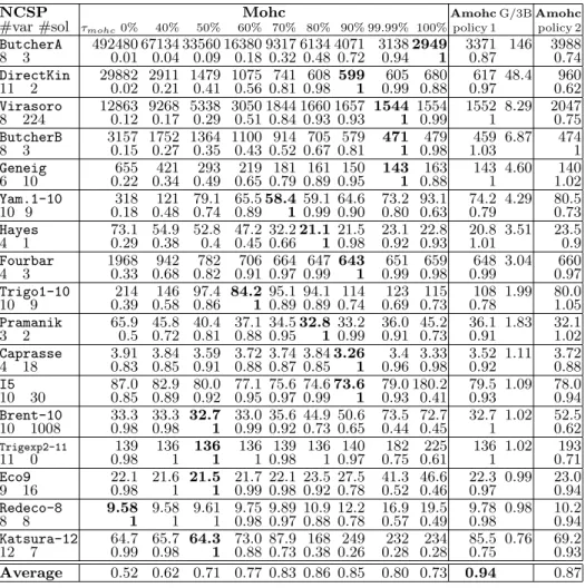
Table 1 contains the main results useful for our analysis. It reports the CPU time (first row of a multi-row) required by the solving strategy described above (based on 3BCID(Mohc)) in function of τmohc. The NCSPs are sorted by
decreas-ing gains in performance of 3BCID(Amohc) w.r.t. 3BCID(HC4) (column G/3B). The entries of columns 2 to 10 also contain (second row of a multi-row) a gain falling in [0, 1]. The gain is T ime(3BCID(Oracle))T ime(3BCID(M ohc)) , where Oracle is a theoretical Mohc variant that would be able to select the best value (yielding the results in bold in the table) for τmohc.
The first 10 columns highlight that the best value of τmohc nearly always
falls in the range [50%, 99.99%]. The value 50% yields always better results than (or similar to) τmohc = 40% or less [1]. Also, τmohc = 99.99% is better than
or similar to 100% (except in ButcherA). Note that Mohc with τmohc = 0% is
identical to HC4 (see Algorithm 1).
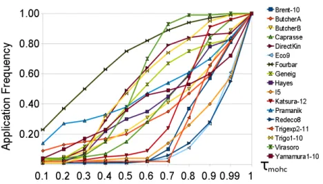
Second, a significant correlation can be observed on Table 1 and on the graphic shown in Fig. 1. The curves show how the application frequency of the monotonicity-based procedures (number of calls(ρmohc[f ]<τmohc)
number of calls(Mohc−Revise) ) evolves when
τmohc increases. (Of course, the frequency becomes 1 when τmohc = 1.) The
correlation can be observed vertically for any value of τmohc, although this is
clearer for intermediate values. For instance, with the abscissa τmohc = 60%,
1 See
www-sop.inria.fr/coprin/logiciels/ALIAS/Benches/benches.html
2 Compared to [2], the NCSP kin1 has been removed because it can be solved with
3BCID(HC4)in less than 100 choice points. ButcherB has been added. ButcherA (with [a] = [−50, −1.1]) and ButcherB (with [a] = [−0.9, 50]) are two sub-instances of the NCSP Butcher. Merlet has manually removed the value a = 1 to avoid a singularity...
6 Ignacio Araya, Gilles Trombettoni, Bertrand Neveu
Table 1.Experimental results. The column G/3B = T ime(3BCID(Amohc))T ime(3BCID(HC4)) highlights the gain of our 3BCID(Amohc) contractor w.r.t. the standard 3BCID(HC4) (column 2).
NCSP Mohc AmohcG/3B Amohc
#var #sol τmohc0% 40% 50% 60% 70% 80% 90% 99.99% 100% policy 1 policy 2
ButcherA 492480 67134 33560 16380 9317 6134 4071 3138 2949 3371 146 3988 8 3 0.01 0.04 0.09 0.18 0.32 0.48 0.72 0.94 1 0.87 0.74 DirectKin 29882 2911 1479 1075 741 608 599 605 680 617 48.4 960 11 2 0.02 0.21 0.41 0.56 0.81 0.98 1 0.99 0.88 0.97 0.62 Virasoro 12863 9268 5338 3050 1844 1660 1657 1544 1554 1552 8.29 2047 8 224 0.12 0.17 0.29 0.51 0.84 0.93 0.93 1 0.99 1 0.75 ButcherB 3157 1752 1364 1100 914 705 579 471 479 459 6.87 474 8 3 0.15 0.27 0.35 0.43 0.52 0.67 0.81 1 0.98 1.03 1 Geneig 655 421 293 219 181 161 150 143 163 143 4.60 140 6 10 0.22 0.34 0.49 0.65 0.79 0.89 0.95 1 0.88 1 1.02 Yam.1-10 318 121 79.1 65.5 58.4 59.1 64.6 73.2 93.1 74.2 4.29 80.5 10 9 0.18 0.48 0.74 0.89 1 0.99 0.90 0.80 0.63 0.79 0.73 Hayes 73.1 54.9 52.8 47.2 32.2 21.1 21.5 23.1 22.8 20.8 3.51 23.5 4 1 0.29 0.38 0.4 0.45 0.66 1 0.98 0.92 0.93 1.01 0.9 Fourbar 1968 942 782 706 664 647 643 651 659 648 3.04 660 4 3 0.33 0.68 0.82 0.91 0.97 0.99 1 0.99 0.98 0.99 0.97 Trigo1-10 214 146 97.4 84.2 95.1 94.1 114 123 115 108 1.99 80.0 10 9 0.39 0.58 0.86 1 0.89 0.89 0.74 0.69 0.73 0.78 1.05 Pramanik 65.9 45.8 40.4 37.1 34.5 32.8 33.2 36.0 45.2 36.1 1.83 32.1 3 2 0.5 0.72 0.81 0.88 0.95 1 0.99 0.91 0.73 0.91 1.02 Caprasse 3.91 3.84 3.59 3.72 3.74 3.84 3.26 3.4 3.33 3.52 1.11 3.72 4 18 0.83 0.85 0.91 0.88 0.87 0.85 1 0.96 0.98 0.92 0.88 I5 87.0 82.9 80.0 77.1 75.6 74.6 73.6 79.0 180.2 79.5 1.09 78.0 10 30 0.85 0.89 0.92 0.95 0.97 0.99 1 0.93 0.41 0.93 0.94 Brent-10 33.3 33.3 32.7 33.0 35.6 44.9 50.6 73.5 72.7 32.7 1.02 52.5 10 1008 0.98 0.98 1 0.99 0.92 0.73 0.65 0.44 0.45 1 0.62 Trigexp2-11 139 136 136 136 139 136 140 182 225 136 1.02 193 11 0 0.98 1 1 1 0.98 1 0.97 0.75 0.61 1 0.71 Eco9 22.1 21.6 21.5 21.7 22.1 23.5 27.5 41.3 46.6 22.3 0.99 23.0 9 16 0.98 1 1 0.99 0.98 0.92 0.78 0.52 0.46 0.97 0.94 Redeco-8 9.58 9.58 9.61 9.75 9.89 10.9 12.2 16.9 19.5 9.78 0.98 10.2 8 8 1 1 1 0.98 0.97 0.88 0.78 0.57 0.49 0.98 0.94 Katsura-12 64.7 65.7 64.3 73.0 87.9 168 249 232 234 85.5 0.76 69.2 12 7 0.99 0.98 1 0.88 0.73 0.38 0.26 0.28 0.28 0.75 0.93 Average 0.52 0.62 0.71 0.77 0.83 0.86 0.85 0.80 0.73 0.94 0.87
the application frequencies of Katsura, Redeco, Eco9, Trigexp2, Brent and I5 are inferior to 10%. It appears that these instances are not very well solved by 3BCID(Mohc) with τmohc= 100% (compared to 3BCID(HC4)). This suggests
that when the application frequency is low (resp. high), τmohc should rather be
tuned to a low (resp. high) value. Intuitively, a high frequency means that a lot of monotonicity-based evaluations produce a sharp interval image, so that Mohc should well exploit these sharp evaluations.
This study has led us to a simple auto-adaptive τmohctuning policy following
three significant choices:
– Since Mohc-Revise exploits the monotonicity of a single function f , there is no reason that τmohcbe the same for all constraints. This prevented the user
Fig. 1.Application frequency of the monot. based procedures in function of τmohc.
from specifying a τmohcparameter for each function f , but this simplification
is no more relevant in an adaptive tuning policy.3
– For any constraint f , τmohc[f ] is fixed to one of both values 50% and 99.99%.
Indeed, if we had an oracle able to select in any instance the best value for τmohc among 50% and 99.99%, the loss in performance w.r.t. an oracle
knowing the best value of τmohc would be only 4%. τmohc = 50% (resp.
99.99%) is generally the most relevant value when the gain in CPU time of 3BCID(Mohc)compared to 3BCID(HC4) is the smallest (resp. greatest). – The application frequency is updated at each node of the search tree. It is
more and more accurate as the number of measurements increases.
These choices lead to the tuning policy 1 based on Algorithm 2. The proce-dure ComputeRhoMohc is run for every constraint at each node of the search tree, before running the contraction procedures. nb calls[f] and nb interes-ting[f], related to a given constraint f , are initialized to 0 before the search. The ratios tau mohc[f] are set to 99.99% during the first 50 nodes before being adjusted in ComputeRhoMohc. The results are not sensitive to a fine tuning of
RHO INTERESTINGandTAU FREQ, empirically fixed to 65% and 10% respectively. The performance of this policy is illustrated by the last line of Table 1. The loss in performance w.r.t. an oracle knowing the best value of τmohc(τmohcbeing
common to all the constraints in a given NCSP) is 6% on average (at worst 25%; around 0% in 7 NCSPs). The obtained average gain (94%) highlights that Amohc is better than any fixed value of τmohc(i.e., 86% for τmohc= 80%). The column
G/3B is also very convincing because 3BCID(Amohc) and 3BCID(HC4) have the same number of parameters, i.e., 0 coming from HC4-Revise and Amohc-Revise.
3 This explains why our auto-adaptive versions of Mohc sometimes (slightly)
8 Ignacio Araya, Gilles Trombettoni, Bertrand Neveu
Algorithm 2 ComputeRhoMohc (in f : a function, V : variables, [V ]: domains)
nb calls[f]++
rho mohc[f]← Diam([f ]M([V ]))
Diam([f ]N([V ])) /* rho mohc[f] is computed */
if rho mohc[f]< RHO INTERESTING then nb interesting[f]++; end if interesting freq← nb interesting[f]nb calls[f]
if nb calls[f]> 50 and interesting freq < TAU FREQ then tau mohc[f]← 50%
else
tau mohc[f]← 99.99% end if
An alternative policy 2 is based on contraction. Each time the monotonicity-based procedures of Algorithm 1 are applied, two ratios of box perimeters are computed: re is the gain in perimeter brought by HC4-Revise w.r.t. the initial
box; rm is the gain brought by MinMaxRevise+MonotonicBoxNarrow w.r.t. the
previous box. If rmis better (enough) than re, then τmohcis slightly incremented;
if reis better than rm, then it is decremented.
As shown in Table 1, the policy 2 is not so bad although less efficient than the policy 1 on average (87%). Unfortunately, this adaptive policy is the worst when Mohc is the most useful (e.g., see ButcherA, DirectKin, Virasoro).
References
1. I. Araya. Exploiting Common Subexpressions and Monotonicity of Functions for
Filtering Algorithms over Intervals. PhD thesis, University of Nice–Sophia, 2010.
2. I. Araya, G. Trombettoni, and B. Neveu. Exploiting Monotonicity in Interval Constraint Propagation. In Proc. AAAI (to appear), 2010.
3. F. Benhamou, F. Goualard, L. Granvilliers, and J.-F. Puget. Revising Hull and Box Consistency. In Proc. ICLP, pages 230–244, 1999.
4. G. Chabert. www.ibex-lib.org, 2010.
5. H. Collavizza, F. Delobel, and M. Rueher. Comparing Partial Consistencies.
Re-liable Comp., 5(3):213–228, 1999.
6. L. Jaulin. Interval Constraint Propagation with Application to Bounded-error Estimation. Automatica, 36:1547–1552, 2000.
7. R. B. Kearfott. Rigorous Global Search: Continuous Problems. Kluwer, 1996. 8. M. Kieffer, L. Jaulin, E. Walter, and D. Meizel. Robust Autonomous Robot
Lo-calization Using Interval Analysis. Reliable Computing, 3(6):337–361, 2000. 9. O. Lhomme. Consistency Tech. for Numeric CSPs. In IJCAI, pages 232–238, 1993. 10. J-P. Merlet. Interval Analysis and Robotics. In Symp. of Robotics Research, 2007. 11. R. E. Moore. Interval Analysis. Prentice-Hall, 1966.
12. M. Rueher, A. Goldsztejn, Y. Lebbah, and C. Michel. Capabilities of Constraint Programming in Rigorous Global Optimization. In NOLTA, 2008.
13. G. Trombettoni and G. Chabert. Constructive Interval Disjunction. In Proc. CP,
LNCS 4741, pages 635–650, 2007.
14. P. Van Hentenryck, L. Michel, and Y. Deville. Numerica : A Modeling Language