HAL Id: hal-02928016
https://hal.archives-ouvertes.fr/hal-02928016
Submitted on 27 Oct 2020
HAL is a multi-disciplinary open access
archive for the deposit and dissemination of
sci-entific research documents, whether they are
pub-lished or not. The documents may come from
teaching and research institutions in France or
abroad, or from public or private research centers.
L’archive ouverte pluridisciplinaire HAL, est
destinée au dépôt et à la diffusion de documents
scientifiques de niveau recherche, publiés ou non,
émanant des établissements d’enseignement et de
recherche français ou étrangers, des laboratoires
publics ou privés.
J. Fisher, M. Sikka, W. Oechel, D. Huntzinger, J. Melton, C. Koven, A.
Ahlström, M. Arain, I. Baker, J. Chen, et al.
To cite this version:
J. Fisher, M. Sikka, W. Oechel, D. Huntzinger, J. Melton, et al.. Carbon cycle uncertainty in
the Alaskan Arctic.
Biogeosciences, European Geosciences Union, 2014, 11 (15), pp.4271-4288.
�10.5194/bg-11-4271-2014�. �hal-02928016�
www.biogeosciences.net/11/4271/2014/ doi:10.5194/bg-11-4271-2014
© Author(s) 2014. CC Attribution 3.0 License.
Carbon cycle uncertainty in the Alaskan Arctic
J. B. Fisher1, M. Sikka1, W. C. Oechel2, D. N. Huntzinger3, J. R. Melton4, C. D. Koven5, A. Ahlström6, M. A. Arain7, I. Baker8, J. M. Chen9, P. Ciais10, C. Davidson11, M. Dietze12, B. El-Masri13, D. Hayes14, C. Huntingford15,
A. K. Jain13, P. E. Levy16, M. R. Lomas17, B. Poulter10, D. Price18, A. K. Sahoo19, K. Schaefer20, H. Tian21, E. Tomelleri22, H. Verbeeck23, N. Viovy10, R. Wania24, N. Zeng25, and C. E. Miller1
1Jet Propulsion Laboratory, California Institute of Technology, 4800 Oak Grove Drive, Pasadena, CA, 91109, USA
2Global Change Research Group, Department of Biology, San Diego State University, San Diego, CA, 92182, USA
and the Department of Environment, Earth, and Ecosystems, The Open University, Milton Keynes, UK
3School of Earth Sciences & Environmental Sustainability, Northern Arizona University, PO Box 5694, Flagstaff, AZ,
86011, USA
4Canadian Centre for Climate Modelling and Analysis, Environment Canada, Victoria, BC, V8W 2Y2, Canada
5Earth Sciences Division, Lawrence Berkeley National Laboratory, Berkeley, CA, 94708, USA
6Department of Physical Geography and Ecosystem Science, Lund University, Sölvegatan 12, 223 62, Lund, Sweden
7School of Geography Earth Sciences and McMaster Centre for Climate Change, McMaster University,
Hamilton, ON, Canada
8Atmospheric Science Department, Colorado State University, Fort Collins, CO, 80523-1371, USA
9Department of Geography, University of Toronto, 100 St. George Street, Toronto, Ontario, M5S 3G3, Canada
10Laboratoire des Sciences du Climat et l’Environnement, Orme des Merisiers, bat. 701 – Point courier 129,
91191 Gif Sur Yvette, France
11Program in Ecology, Evolution, and Conservation Biology, University of Illinois at Urbana-Champaign, 505 S. Goodwin
Ave, Urbana, IL, 61801, USA
12Department of Earth and the Environment, Boston University, 675 Commonwealth Ave, Boston, MA, 02215, USA
13Department of Atmospheric Sciences, University of Illinois, Urbana, IL, 61801, USA
14Climate Change Science Institute and Environmental Sciences Division, Oak Ridge National Laboratory, Oak Ridge, TN,
37831-6301, USA
15Centre for Ecology and Hydrology, Benson Lane, Wallingford, OX10 8BB, UK
16Centre for Ecology and Hydrology, Penicuik, Midlothian, EH26 0QB, UK
17Centre for Terrestrial Carbon Dynamics, University of Sheffield, Dept. of Animal & Plant Sciences, Western Bank,
Sheffield, S10 2TN, UK
18Natural Resources Canada, Northern Forestry Centre, 5320 – 122 Street Northwest, Edmonton, Alberta, T6H 3S5, Canada
19Department of Civil and Environmental Engineering, Princeton University, Princeton, New Jersey, 08544, USA
20National Snow and Ice Data Center, Cooperative Institute for Research in Environmental Sciences, University of Colorado
at Boulder, Boulder, CO, 80309, USA
21School of Forestry and Wildlife Sciences, Auburn University, 602 Duncan Drive, Auburn, AL, 36849, USA
22Biogeochemical Model-Data Integration Group, Max Planck Institute for Biogeochemistry, Hans-Knöll-Str. 10, 07745,
Jena, Germany
23Laboratory of Plant Ecology, Faculty of Bioscience Engineering, Ghent University, Coupure Links 653,
9000 Ghent, Belgium
24Institut des Sciences de l’Evolution (UMR5554, CNRS), Université Montpellier 2, Place Eugène Bataillon,
34090 Montpellier, France
25Department of Atmospheric and Oceanic Science, University of Maryland, 2417 Computer and Space Sciences Building,
College Park, MD, 20742-2425, USA
Received: 22 January 2014 – Published in Biogeosciences Discuss.: 20 February 2014 Revised: 17 June 2014 – Accepted: 22 June 2014 – Published: 14 August 2014
Abstract. Climate change is leading to a disproportionately large warming in the high northern latitudes, but the magni-tude and sign of the future carbon balance of the Arctic are highly uncertain. Using 40 terrestrial biosphere models for the Alaskan Arctic from four recent model intercomparison projects – NACP (North American Carbon Program) site and regional syntheses, TRENDY (Trends in net land atmosphere carbon exchanges), and WETCHIMP (Wetland and Wetland
CH4 Inter-comparison of Models Project) – we provide a
baseline of terrestrial carbon cycle uncertainty, defined as the multi-model standard deviation (σ ) for each quantity that follows. Mean annual absolute uncertainty was largest for
soil carbon (14.0 ± 9.2 kg C m−2), then gross primary
pro-duction (GPP) (0.22 ± 0.50 kg C m−2yr−1), ecosystem
res-piration (Re) (0.23 ± 0.38 kg C m−2yr−1), net primary pro-duction (NPP) (0.14 ± 0.33 kg C m−2yr−1), autotrophic res-piration (Ra) (0.09 ± 0.20 kg C m−2yr−1), heterotrophic res-piration (Rh) (0.14 ± 0.20 kg C m−2yr−1), net ecosystem
ex-change (NEE) (−0.01 ± 0.19 kg C m−2yr−1), and CH4 flux
(2.52 ± 4.02 g CH4m−2yr−1). There were no consistent spa-tial patterns in the larger Alaskan Arctic and boreal regional carbon stocks and fluxes, with some models showing NEE for Alaska as a strong carbon sink, others as a strong car-bon source, while still others as carcar-bon neutral. Finally, AmeriFlux data are used at two sites in the Alaskan Arc-tic to evaluate the regional patterns; observed seasonal NEE was captured within multi-model uncertainty. This assess-ment of carbon cycle uncertainties may be used as a base-line for the improvement of experimental and modeling ac-tivities, as well as a reference for future trajectories in car-bon cycling with climate change in the Alaskan Arctic and larger boreal region.
1 Introduction
Changes in climate have led to a relatively large warming in the high northern latitudes, that is, the Arctic, due to a temperature–albedo feedback from the loss of snow and sea ice, as well as the breakdown of polar near-surface temper-ature inversions (i.e., more water vapor, leading to greater greenhouse gas effect; also, changes in cloud cover) (Cess et al., 1991; Chapin et al., 2005; Chapman and Walsh, 1993, 2007; IPCC, 2007; McGuire et al., 2006; Overpeck et al., 1997; Serreze et al., 2000; Walsh et al., 2002). Throughout
the Holocene, Arctic ecosystems have absorbed more CO2
from the atmosphere through photosynthesis than have emit-ted back to the atmosphere through respiration (Kuhry et al., 2009; Marion and Oechel, 1993; Oechel et al., 1993; Ping et
al., 2008; Tarnocai, 2006). The pervasive cold and wet condi-tions in the Arctic have limited the decay of soil organic car-bon, resulting in the accumulation of carbon on the order of
35–70 kg C m−2total (∼ 25 % of the global soil organic
car-bon pool; Mishra and Riley, 2012; Ping et al., 2008; Tarnocai et al., 2009) stored above and beneath the permafrost and in peatlands over centuries to millennia.
Warming, however, is thawing permafrost and changing the soil water balance and water table, resulting in the re-lease of previously stored soil carbon to the atmosphere,
thereby exacerbating the atmospheric CO2impact on the
cli-mate (Belshe et al., 2013, 2012; Burke et al., 2012; Chris-tensen et al., 2004; Hayes et al., 2011; Koven et al., 2011; McGuire et al., 2009; Natali et al., 2012, 2014; Oechel et al., 1993, 2000; Oechel and Vourlitis, 1994; Schaefer et al., 2011; Schuur and Abbott, 2011; Schuur et al., 2008, 2009, 2013; Zimov et al., 2006). Alternatively, warming acceler-ates soil decomposition, which may release nutrients into the nutrient-limited ecosystems, and, combined with more favorable growing conditions and additional growing days, drive the Arctic towards a carbon sink regime (Mack et al., 2004; Qian et al., 2010; Sistla et al., 2013). While point-based measurements in the Alaskan Arctic indicate that it
is currently a net CO2source to the atmosphere (Oechel et
al., 1993, 2000, 2014; Oechel and Vourlitis, 1994), given the lack of continuous, large-scale observations of the
Arc-tic net ecosystem exchange (NEE) of CO2it is still
impossi-ble to determine with certainty whether or not the Arctic is
a net carbon sink or source, let alone the future Arctic CO2
flux magnitude or even sign of flux (Hinzman et al., 2005; McGuire et al., 2009, 2012).
A number of new field campaigns aim to address these uncertainties: the Carbon in Arctic Reservoirs Vulnerabil-ity Experiment (CARVE; NASA) (Miller et al., 2010), the Arctic Boreal Vulnerability Experiment (ABoVE) (Goetz et al., 2011), and the Next Generation Ecological Experiment (NGEE Arctic) (Wullschleger et al., 2011). All of these cam-paigns focus on Alaskan Arctic and boreal zones as the major region of study, aiming to reduce uncertainty in the Arctic and boreal carbon cycle. However the uncertainty has not been well quantified. McGuire et al. (2012) provided the closest solution to this problem, compiling global and re-gional land and atmospheric models to quantify pan-Arctic carbon budgets, and our paper builds on this groundbreaking effort with a narrowed regional and topical focus on Alaskan Arctic and boreal carbon uncertainties, sensitivities, and spa-tial patterns. Our analysis is specifically designed for appli-cation to these Alaskan field campaigns, which require jus-tification for geographic sampling decisions needed across Alaska as a single domain; we provide the spatial distribution
of uncertainties where McGuire et al. did not. We also in-clude in situ measurements from AmeriFlux sites within the Alaskan Arctic for quantitative comparison to simulation re-sults. Moreover, we expand the uncertainty quantification to four times as many carbon cycle variables across four times as many terrestrial biosphere models, necessary for under-standing how uncertainty values are constructed in global cli-mate change projections (Friedlingstein et al., 2006; IPCC, 2007).
This effort is made possible by recent terrestrial bio-sphere model intercomparison projects (MIPs) – TRENDY (Piao et al., 2013), the North American Carbon Program (NACP) regional and site syntheses (Hayes et al., 2012; Huntzinger et al., 2012; Schwalm et al., 2010), and the
Wet-land and WetWet-land CH4 Inter-comparison of Models Project
(WETCHIMP) (Melton et al., 2013; Wania et al., 2013) – which have organized a multitude of international mod-eling teams to contribute their latest model estimates us-ing both common forcus-ing data (i.e., TRENDY, NACP site, WETCHIMP) as well as a mixture of different forcing data (i.e., NACP regional). These MIPs extended from global (TRENDY, WETCHIMP) to regional (NACP regional) to site level (NACP site) domains. The models included in these MIPs form the scientific community’s understanding of global carbon cycle processes, with large uncertainties globally stemming from large uncertainties regionally and locally, particularly for the Arctic. The scientific commu-nity has been focused on diagnoses of individual model skill, benchmarking, and suggestions for improvements, and we defer to other papers for such analyses (Huntzinger et al., 2012; Schaefer et al., 2012; Schwalm et al., 2010).
Here, we use the between-model variability from these MIPs to define the uncertainties in the Alaskan Arctic and boreal carbon cycle. This total uncertainty integrates both structural uncertainty of land-surface physics among models as well as inherent parametric uncertainty introduced within models, and uncertainty from forcing data. Finally, to under-stand the absolute skill of model estimates, we evaluate the performance of the models against in situ measurements of carbon fluxes at AmeriFlux sites along the Alaskan North Slope. The objective of this analysis is to compile and quan-tify the predictive uncertainty in terrestrial carbon cycle dy-namics applied to the Alaskan Arctic and boreal region to provide a baseline of uncertainty and spatial maps geolocat-ing this uncertainty for current and future field campaigns in the region. The primary focus of the uncertainty calculations is on the Alaskan North Slope or “Alaskan Arctic”; however, we also provide maps of the larger Arctic and boreal region encompassing the entire state of Alaska.
2 Methods
2.1 Regional level
We used 14 NACP regional synthesis models, 9 TRENDY models, and 7 WETCHIMP models for regional carbon flux and/or stock estimates.
The 14 NACP regional synthesis models include (Ta-ble 1): BEPS (Chen et al., 1999), CanIBIS (El Maa-yar et al., 2002), CASA-GFED (van der Werf et al., 2004), CASA-TRANSCOM (Randerson et al., 1997), CLM-CASA (Randerson et al., 2009), CLM4-CN (Thorn-ton et al., 2007), DLEM (Tian et al., 2010), ISAM (Jain and Yang, 2005), LPJwsl (Sitch et al., 2003), MOD17 (Zhao et al., 2005), ORCHIDEE (Krinner et al., 2005), SiB3 (Baker et al., 2008), TEM6 (Hayes et al., 2011), and VEGAS2 (Zeng et al., 2005). Model out-put for the NACP regional synthesis was downloaded from: ftp://nacp.ornl.gov/synthesis/2008/firenze/continental/ 1_continental_data_model_inventory.html. All NACP
re-gional synthesis models were provided at 1◦×1◦spatial
res-olution.
The nine TRENDY models include: CLM4-CN (Thorn-ton et al., 2007), HYLAND (Levy et al., 2004), LPJwsl (Sitch et al., 2003), LPJ-GUESS (Smith et al., 2001), OCN (Zaehle et al., 2010), ORCHIDEE (Krinner et al., 2005), SDGVM (Cramer et al., 2001), TRIFFID (Clark et al., 2011), and VEGAS (Zeng et al., 2005). Model output for TRENDY was downloaded from: http://www-lscedods.cea. fr/invsat/RECCAP/. Output from multiple versions of the same model were sometimes available; in these cases, we used output only from the most recent version. We primar-ily used the version S2 runs, which correspond to
simultane-ously meteorological forcings and atmospheric CO2
concen-tration variation following 20th century increases, with dis-turbance turned off and a constant land use mask. We also
used version S1, which varies only CO2, to evaluate
sen-sitivities to CO2 and climate. Model LPJ-GUESS, LPJwsl,
and ORCHIDEE were provided at 0.5◦×0.5◦ spatial
res-olution; CLM4CN at 1.875◦×2.5◦ spatial resolution;
VE-GAS at 2.5◦×2.5◦spatial resolution; and HYLAND, OCN,
SDGVM, and TRIFFID at 2.5◦×3.75◦spatial resolution.
The seven WETCHIMP models include: CLM4Me (Ri-ley et al., 2011b), DLEM (Tian et al., 2010), LPJ-Bern (Spahni et al., 2011), LPJ-WHyMe (Wania et al., 2010), LPJwsl (Sitch et al., 2003), ORCHIDEE (Krinner et al., 2005), and SDGVM (Cramer et al., 2001). Model output for WETCHIMP was downloaded from: http://arve.unil.ch/ pub/wetchimp. Output from six experiments were available (Melton et al., 2013), but we used only experiment 2, corre-sponding to the transient simulation from 1901 to 2009
us-ing observed climate and CO2values. Models DLEM,
LPJ-Bern, LPJ-WHyMe, SDGVM, and LPJwsl were provided at
0.5◦×0.5◦spatial resolution; ORCHIDEE at 1◦×1◦spatial
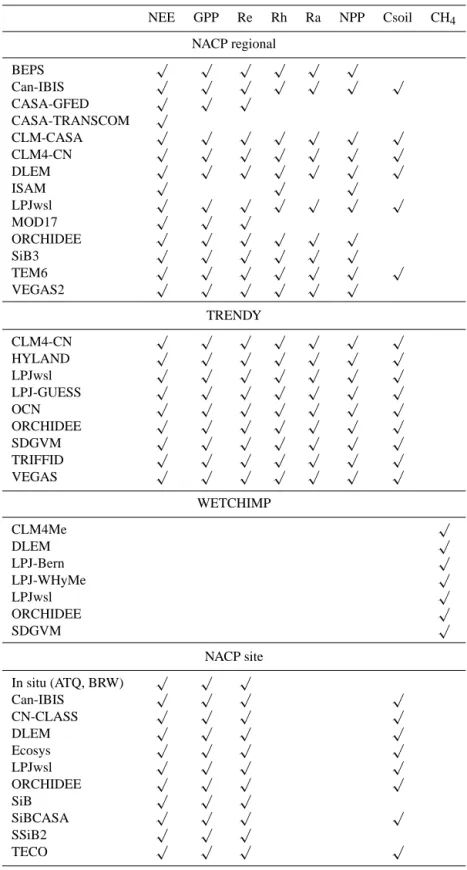
Table 1. Models and carbon output variables. NEE GPP Re Rh Ra NPP Csoil CH4 NACP regional BEPS √ √ √ √ √ √ Can-IBIS √ √ √ √ √ √ √ CASA-GFED √ √ √ CASA-TRANSCOM √ CLM-CASA √ √ √ √ √ √ √ CLM4-CN √ √ √ √ √ √ √ DLEM √ √ √ √ √ √ √ ISAM √ √ √ LPJwsl √ √ √ √ √ √ √ MOD17 √ √ √ ORCHIDEE √ √ √ √ √ √ SiB3 √ √ √ √ √ √ TEM6 √ √ √ √ √ √ √ VEGAS2 √ √ √ √ √ √ TRENDY CLM4-CN √ √ √ √ √ √ √ HYLAND √ √ √ √ √ √ √ LPJwsl √ √ √ √ √ √ √ LPJ-GUESS √ √ √ √ √ √ √ OCN √ √ √ √ √ √ √ ORCHIDEE √ √ √ √ √ √ √ SDGVM √ √ √ √ √ √ √ TRIFFID √ √ √ √ √ √ √ VEGAS √ √ √ √ √ √ √ WETCHIMP CLM4Me √ DLEM √ LPJ-Bern √ LPJ-WHyMe √ LPJwsl √ ORCHIDEE √ SDGVM √ NACP site In situ (ATQ, BRW) √ √ √ Can-IBIS √ √ √ √ CN-CLASS √ √ √ √ DLEM √ √ √ √ Ecosys √ √ √ √ LPJwsl √ √ √ √ ORCHIDEE √ √ √ √ SiB √ √ √ SiBCASA √ √ √ √ SSiB2 √ √ √ TECO √ √ √ √
Notes: NEE includes NBP (all TRENDY models except HYLAND) and NEP (NACP regional: BEPS, Can-IBIS, CLM-CASA, CLM4-CN, VEGAS2; TRENDY: HYLAND). Re may be calculated from Rh + Ra (e.g., NACP regional) or NEE-GPP (all NACP regional except CASA-TRANSCOM and ISAM; all TRENDY). Ra may be calculated from NEE-GPP-Rh (NACP regional: BEPS, CLM-CASA, CLM4-CN, ORCHIDEE, TEM6; TRENDY: HYLAND, ORCHIDEE, VEGAS). NPP may be calculated from GPP-Ra (TRENDY: LPJ-GUESS).
49 941
Figure 1. Map of the Alaskan Arctic North Slope delineation, and the two AmeriFlux sites used 942
in this study (Atqasuk: ATQ; Barrow: BRW).
943 Figure 1. Map of the Alaskan Arctic North Slope delineation, andthe two AmeriFlux sites used in this study (Atqasuk: ATQ; Barrow:
BRW).
Variables assessed for NACP regional and TRENDY in-cluded: NEE, gross primary production (GPP), heterotrophic respiration (Rh), autotrophic respiration (Ra), net primary production (NPP), and soil carbon stock (Csoil). Some mod-els provided GPP and NPP, but not Ra, while others provided GPP and Ra, but not NPP, so we were able to calculate the
missing term in those equations with one unknown. CH4was
provided only from WETCHIMP models, and this is solely what we used the WETCHIMP models for. Most variables were identical across NACP regional and TRENDY, except
that the net CO2flux was reported as net biome production
(NBP) for TRENDY (and net ecosystem production, NEP, for HYLAND only), whereas oppositely it was reported as NEE for NACP regional. We reversed the sign for TRENDY (and converted time units of seconds to months) to equate
the CO2flux between both MIPs, though we note that
tech-nically NBP should include additional fluxes from fire and other disturbances as well as lateral carbon transport that NEE would not include. Models LPJwsl and VEGAS from TRENDY were not converted because their values were al-ready in the units of NACP. Models HYLAND and SDGVM
in TRENDY reported net CO2 flux values in the incorrect
sign so we reversed the sign.
We created a half-degree resolution mask of the state of Alaska and a mask of the North Slope (Fig. 1) used to clip from the global (TRENDY) and North America (NACP re-gional) model output. We transformed the masks to match the different native resolutions of the models. We produced mean annual maps for the state of Alaska for NEE, GPP, Rh, Ra, NPP, and Csoil by averaging the available monthly model output and preserving the native spatial resolution for each model. We set a uniform color scale bar for between-model visual comparison (rather than individual scale bars for each model, which would highlight within-model spatial variabil-ity). However, in some the range was effectively truncated
due to some large values beyond our set minimum/maximum of the scale; in other cases the minimum/maximum was wider than a given model’s range, so spatial variation within that model may be difficult to visualize.
We produced maps for the multi-model mean ( ¯x) and
stan-dard deviation (σ ) from the individual mean annual maps. Given non-uniform spatial resolutions across models, we
present the multi-model ( ¯x) and σ at the finest resolution
(i.e., 0.5◦). We arithmetically downscaled all models with
coarser resolutions to 0.5◦. Pixels that overlapped with one
another across models were used to calculate the individ-ual half-degree pixel averages. Finally, we re-applied the
half-degree mask of Alaska to the resultant multi-model ( ¯x)
and σ maps (i.e., removing newly added beyond-coastal pix-els from the combination of some wider-extent, coarse-scale
models). The multi-model ( ¯x) color scale bar was set equal
to that of the individual model maps; the color scale bar for the σ was set differently, tailored to the range of the σ . We also generated a time series plot from the spatial mean of all pixels in the Alaskan Arctic for each month for each model (except for Csoil, which did not vary temporally over our time domain).
While the MIPs enable us to conduct an extensive analysis, they also impose some limitations: (i) not all possible Ter-restrial Biosphere Models (TBMs) are included in the MIPs (e.g. there are TBMs used in the scientific community that were not contributed); (ii) the models are not completely in-dependent from one another, at times sharing similar physics for some processes, and with some contributing to multi-ple MIPs; (iii) the forcing data accuracy and variability were not assessed (though they were originally cross-checked and considered the best available); and (iiv) some models have more sophisticated representation of the biophysical pro-cesses important in the Arctic than others (though all TBMs produce Arctic estimates). Nonetheless, the data available for this analysis provide a representative range of information for calculating a baseline of uncertainty and variability in key environmental variables of the Alaskan Arctic. Overcoming some of the above limitations would allow improvements in the estimation of our baseline uncertainty.
2.2 Site level
We used model output from 10 NACP site synthesis mod-els, which include: CanIBIS (El Maayar et al., 2002), CN-CLASS (Arain et al., 2006), DLEM (Tian et al., 2010), Ecosys (Grant et al., 2009), LPJwsl (Sitch et al., 2003), ORCHIDEE (Krinner et al., 2005), SiB (Baker et al., 2008), SiBCASA (Schaefer et al., 2008), SSiB2 (Xue et al., 1991), and TECO (Weng and Luo, 2008). Model output for the NACP site synthesis was downloaded from: http:// isynth-site.pbworks.com/w/page/9422807/FrontPage. Mod-els were provided with in situ measured forcing data for each site to produce site level (e.g., point) model estimates.
In situ data from the Alaskan North Slope
Atqa-suk (70.4696◦N, −157.4089◦W) and Barrow (71.3225◦N,
−156.6259◦W) sites (Kwon et al., 2006) (Fig. 1) were
mod-ified from http://www.fluxdata.org (Agarwal et al., 2010) by adding the self-heating correction to all Atqasuk data (the “Burba” correction; Oechel et al., 2014). Data used for 2006 were from Oechel et al. (2014), which used the same correc-tion as for the other available years. The in situ sites are part of the regional AmeriFlux network and global FLUXNET network where tower-based eddy covariance fluxes and mi-crometeorological variables are measured (Baldocchi, 2008). Half-hourly data were used to compute mean diurnal (from mean hourly) and seasonal (from mean monthly) cycles.
Atqasuk consists of moist-wet coastal sedge tundra and moist tussock tundra surfaces (e.g., Eriophorum vaginatum) in the well-drained upland (Oechel et al., 2014). Barrow con-sists of undisturbed wet-moist coastal sedge tundra types, multiple ice wedges, drained lake tundra land forms, and is located 2 km south of the Arctic Ocean and 100 km north of Atqasuk (Zona et al., 2010); the Alaskan coastal plain encompassing Barrow was generally not glaciated during the last period of glaciation. Atqasuk’s more continental cli-mate and sandy substrate make a useful contrast with con-ditions at Barrow (Kwon et al., 2006). Another Alaskan AmeriFlux eddy covariance ground site, Ivotuk, was op-erational; however, site-level model simulations were not available for this site.
To maintain consistency for fair comparison, when one data point was missing for either model or site, we removed all data points for that time step for all models and measure-ments; thus, the averages shown are not necessarily “true” averages for each model or measurements. Days were ex-cluded if fewer than 12 h of data were available. We used the available in situ data to define our site level time do-main: 2003–2006 for Atqasuk and 1998–2002 for Barrow. In situ data for Barrow were available only during the growing season (northern summer) for most years. Variables assessed included: NEE, GPP, Re, and Csoil. NACP processed files for NEE, GPP, and Re were used for analysis; original/raw NetCDF (Network Common Data Form; nc) files were used for all other variables. Raw files for ORCHIDEE had to be time shifted by 9 h; leap years were adjusted for ORCHIDEE and LPJwsl. Not all models or sites provided data for all vari-ables. Models did not provide diurnally or seasonally varying site level Csoil so analysis of Csoil was done at the annual timescale only.
To link the site measurements to the regional model pat-terns, we evaluated the correlation structure between NEE and GPP or Re at the sites versus the region. That is, we
cal-culated the r2for NEE vs. GPP and NEE vs. Re. This was
done for the site measurements and for each model at the re-gional level. We then evaluated how well the rere-gional models matched the site level correlation patterns.
To provide a spatial picture of how representative the sites are to the larger region, we constructed statewide
site representativeness maps based on statewide spatially explicit climatology using the incremental analysis updates (IAU) 2-D atmospheric single level diagnostics (near surface air temperature) and IAU 2-D land-surface diagnostics (precipitation) from the Modern Era Retrospective Analysis for Research and Applications (MERRA) generated by NASA’s Global Modeling and Assimilation Office (GMAO)
at 0.5 × 0.66◦ resolution (Rienecker et al., 2011). MERRA
data were downloaded from: http://disc.sci.gsfc.nasa.gov/
daac-bin/DataHoldings.pl?LOOKUPID_List=MAT1NX∗∗∗
(where∗∗∗is “SLV” or “LND” for air temperature and
pre-cipitation, respectively). We compared the mean daily time series of site level air temperature and precipitation for 2001 (i.e., the year that both sites overlapped, for comparison; flux data were not available at Atqasuk for 2001) against the corresponding time series of the MERRA data for each pixel
in Alaska, computing the correlation coefficient (r2) for
each pixel (e.g., variability representativeness). We removed MERRA data for time steps where there were data gaps from the in situ data. We adjusted the time zones between the in situ data and MERRA (i.e., Alaskan Standard Time, AST; Greenwich Mean Time, GMT, respectively) to match. We converted units of air temperature from Kelvin (MERRA) to Celsius (in situ), and units of precipitation from mm (in situ)
to kg m−2s−1(MERRA) to match.
3 Results
The Results are partitioned into five sub-sections: (I) spatial variability; (II) temporal variability; (III) an integrated sum-mary; (IV) sensitivity analysis; and (V) site level evaluation.
3.1 Spatial variability in carbon
The spatial patterns in mean annual NEE for statewide Alaska (Arctic and boreal region) varied widely among the models, essentially showing no consistency, with almost all patterns having at least one other model showing the oppo-site pattern (Fig. 2; data for a single year, 2003, are shown for example, though these relative patterns remain for other years). Some models showed the entire region as a strong carbon sink, others as a strong carbon source, while still others as close to carbon neutral. Some models showed a large portion of the region as a carbon sink with the rest of the state a carbon source; other models showed the oppo-site pattern of source and sink distribution. It is also visu-ally apparent that the spatial resolutions vary widely among
models (i.e., 0.5 × 0.5◦–2.5 × 3.75◦). The multi-model mean
annual NEE for Alaska shows the region as largely carbon neutral (Fig. 3a). This contradicts some observations that
show the region to be an overall source of CO2to the
atmo-sphere (Oechel et al., 2000, 2014). The multi-model annual NEE σ for Alaska shows model agreement or disagreement
50 CAN-‐IBIS (NACP) DLEM (NACP) MOD17 (NACP) TEM6 (NACP) CASA-‐GFED (NACP) HYLAND (TRENDY) OCN (TRENDY) TRIFFID (TRENDY) CASA-‐TRANSCOM (NACP) ISAM (NACP) ORCHIDEE (NACP) VEGAS (TRENDY) CLM-‐CASA (NACP) LPJ-‐GUESS (TRENDY) ORCHIDEE (TRENDY) VEGAS2 (NACP) CLM4-‐CN (NACP) LPJwsl (NACP) SDGVM (TRENDY) BEPS (NACP) CLM4-‐CN (TRENDY) LPJwsl (TRENDY) SiB3 (NACP) (sink) (source) 944
Figure 2. Mean annual (2003) net CO2 flux for Alaska. Model output was part of the TRENDY
945
(common forcing) and NACP Regional (variable forcing) syntheses. 946
−0.005 0.005
CO2 Flux (kg C m−2 month−1)
Figure 2. Mean annual (2003) net CO2flux for Alaska. Model output was part of the TRENDY (common forcing) and NACP regional (variable forcing) syntheses.
distributed throughout the region, with greater agreement in boreal regions than in tundra regions (Fig. 3b).
In the Supplement figures, we provide the same spatial di-agnostics for the carbon components that comprise NEE, that is, GPP, NPP, Rh, and Ra (Figs. S1–8).
For CH4, fluxes were primarily present and largest in
the southernmost regions of Alaska (Figs. 4 and 5a). Most model disagreement was along the southwest Alaska Penin-sula/southeast Alaska Panhandle (Fig. 5b). There was also
significant disagreement as to whether or not CH4fluxes
oc-cur at all in the interior of Alaska. Models such as DLEM (Tian et al., 2014) and ORCHIDEE estimated no interior
CH4flux whereas LPJ-WHyMe, LPJ-Bern, and SDGVM
es-timated moderate to high fluxes of CH4. The spatial
differ-ences in CH4fluxes among models are primarily due to
dif-ferences in wetland location schemes in the models, soil tem-perature and freeze/thaw sensitivity, and the magnitude of the
51
a) Multi-‐Model (23) Mean CO2 Flux
b) Standard Deviation
Figure 3. NACP and TRENDY multi-model (n=23) net CO2 flux for 2003 a) mean, and b)
947
standard deviation.
948
Figure 3. NACP and TRENDY multi-model (n = 23) net CO2flux for 2003 (a) mean, and (b) standard deviation.
fluxes is due to the vegetation dynamics and soil maps used in the models (Olefeldt et al., 2013). Models LPJ-WHyMe and LPJ-Bern both used the same peatland database to de-termine peatland locations (the two models also contain
sim-ilar code structures), which gives them more central CH4
-producing regions, though they are not identical because of differences in inundation thresholds and wet mineral soils
leading to CH4fluxes. Models DLEM, ORCHIDEE, LPJwsl,
and CLM4Me all are driven with or are parameterized from an inundation data set, which provided a bias away from in-terior CH4-producing regions. Model SDGVM calculates the wetlands extent independently, somewhat similar to the wet soils parameterization in LPJ-Bern.
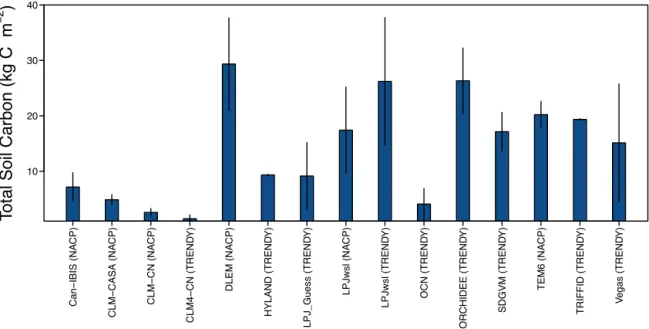
Total soil carbon for the Alaskan Arctic (North Slope)
var-ied from 1.4 to 29.3 kg C m−2across models (Fig. 6), with a
multi-model mean of 14.0 kg C m−2and σ of 9.2 kg C m−2.
We provide the spatial diagnostics for soil carbon in Supple-ment Fig. S9 (individual models) and Fig. S10 (multi-model mean and standard deviation). There was no clear spatial pat-tern similarity across models in soil carbon, with the greatest multi-model uncertainty throughout the permafrost areas in the north.
3.2 Temporal variability in carbon
The mean Alaskan Arctic (North Slope) time-varying NEE for each model was generally similar in timing across mod-els, showing carbon sinks in the short growing season, sepa-rated by carbon sources in the winter that represented lower rates but over a longer period (Fig. 7; we show two years for comparison, 2002–2003, though the relative patterns remain for other years). The model de-trended (from the
multi-model mean) σ was 0.01 kg C m−2yr−1. The multi-model
mean month of greatest CO2 uptake was July, with a σ of
0.5 months.
In the Supplement figures, we provide the same time series plots for the carbon components that comprise NEE (GPP, NPP, Rh, and Ra; Figs. S11–14). Of particular note is the
considerable variability among models in their estimates of Rh during the winter (November–March) (Fig. S13), when all other flux components minimized to zero during this “dor-mant” period (i.e., November–March). This pattern was cor-roborated by a recent analysis of winter Rh (between 0–20 % of annual Rh) in similar ecosystems (Wang et al., 2011). The winter carbon source is also seen as integrated into the time series of NEE in Fig. 7.
The time series for CH4 in the Alaskan Arctic (North
Slope) showed similar temporal patterns for most of the
mod-els with CH4 flux emissions year round for many models
(Fig. 8). The multi-model mean month of greatest CH4
emis-sion was August for both years, with a σ of 1.4 months. The
variability in timing of greatest CH4 emission was nearly
three times that of greatest CO2uptake, indicating large
un-certainty in CH4flux timing relative to that of CO2,
presum-ably because the climatic controls on photosynthesis (light
and temperature) constrain the period of greatest CO2uptake
more narrowly than the combination of temperature and soil moisture that would be likely to affect the modeled seasonal
maximum CH4release.
Seasonal patterns were negligible for soil carbon (e.g., relatively constant throughout each year) so these are not shown.
3.3 Summary of carbon uncertainties
From a total carbon perspective, the largest quantity of ab-solute σ for the Alaskan Arctic (North Slope) was in soil
carbon, followed by GPP, Re, NPP, Ra, Rh, NEE, and CH4
(Fig. 9). Proportionally for the gross fluxes (i.e., exclud-ing NEE and NPP), the largest relative (as opposed to ab-solute) uncertainty was in Ra at 226 % (0.09 ± 0.20 kg C m−2yr−1), GPP at 225 % (0.22 ± 0.50 kg C m−2yr−1), Re
at 169 % (0.23 ± 0.38 kg C m−2yr−1), CH4 flux at 160 %
(2.52 ± 4.02 g CH4m−2yr−1), Rh at 149 % (0.14 ± 0.20 kg
52
CLM4Me LPJ-‐Bern LPJwsl SDGVM DLEM LPJ-‐WhyMe ORCHIDEE949
Figure 4. Mean annual (2003) net CH
4flux for Alaska. Model output was part of the
950
WETCHIMP model intercomparison project.
951
0 0.4
CH4 Flux (g CH4 m−2 month−1)
Figure 4. Mean annual (2003) net CH4flux for Alaska. Model output was part of the WETCHIMP model intercomparison project.
Figure 5. WETCHIMP multi-model (n = 7) net CH4flux for 2003 (a) mean and (b) standard deviation.
3.4 Site level evaluation
To compare against measured carbon fluxes and soil carbon stocks, we present results from two sites located in the North Slope of Alaska – Atqasuk and Barrow – where a subset of models (NACP site) were run using in situ forcing data. First, to understand how representative the sites were to the larger region in lieu of a comprehensive spatial sampling study, we conducted a comparison of climatology at each site to that in each pixel, encompassing all of Alaska (Fig. S15). The expectation was that pixels closer to the sites would exhibit greater similarity in climatology, and this similarity would degrade following some linear or non-linear pattern within increasing distance away from the sites. Variability in cli-mate was better represented in Atqasuk than Barrow rela-tive to the wider region, which reinforces the conclusion that Atqasuk represents a more continental climate than does Bar-row (Kwon et al., 2006).
Relative to in situ measured NEE, models did not capture the seasonal cycle well at either site (Fig. 10ab). Nonethe-less, observed NEE tended to be contained within the
multi-model uncertainty, which gives some indication that the re-gional uncertainty (e.g., in Fig. 7) may also bracket the true
signal of NEE. The mean model seasonal r2 was 0.13 at
Atqasuk and 0.50 at Barrow (both-site mean: 0.32). The mean model seasonal RMSE was more similar than the
r2 between sites, with 0.41 µmol CO2m−2s−1 at
Atqa-suk and 0.46 µmol CO2m−2s−1at Barrow (both-site mean:
0.44 µmol CO2m−2s−1). The multi-model monthly mean
NEE and σ were −0.03 ± 0.64 µmol CO2m−2s−1 at
Atqa-suk and −0.04 ± 0.54 µmol CO2m−2s−1at Barrow.
The greatest observed CO2 uptake at Atqasuk was
typ-ically in June, whereas the multi-model mean placed the
greatest CO2uptake in July. For Barrow, the month of
great-est observed CO2 uptake was typically July or August, and
the multi-model mean tended to capture that timing accu-rately. This evaluation may extend into the regional analy-sis, indicating that the models likely capture the peak sea-sonal NEE timing, though possibly with a slight time lag. It is noted that the “observed” data presented here are not necessarily accurate representations of the actual in situ
54
954
Figure 6. Mean annual Alaskan Arctic (North Slope) total soil carbon with spatial standard
955
deviations.
956
Can − IBIS (NA CP) CLM − CASA (NA CP) CLM − CN (NA CP) CLM4 − CN (TREND Y) DLEM (NA CP) HYLAND (TREND Y) LPJ_Guess (TREND Y) LPJwsl (NA CP) LPJwsl (TREND Y) OCN (TREND Y) ORCHIDEE (TREND Y) SDGVM (TREND Y) TEM6 (NA CP) TRIFFID (TREND Y) V egas (TREND Y) 10 20 30 40Total Soil Carbon (kg C
m
−
2
)
Figure 6. Mean annual Alaskan Arctic (North Slope) total soil carbon with spatial standard deviations.
957
Figure 7. Mean monthly net CO2 flux for the Alaskan Arctic (North Slope), showing two years,
958
for example (2002-2003). NACP models are shown as solid lines, and TRENDY models as
959
dashed lines. The gray area is the multi-model standard deviation.
960
2002 2003 −0.05 0.00 0.05 0.10Year
C
O
2Flux (kg C
m
− 2m
o
n
th
− 1)
BEPS Can−IBIS CASA−GFED CASA−Transcom CLM−CASA CLM−CN DLEM ISAM LPJwsl MOD 17+ ORCHIDEE SiB3 TEM6 VEGAS2 CLM4−CN LPJ_Guess LPJwsl OCN ORCHIDEE TRIFFID VegasFigure 7. Mean monthly net CO2flux for the Alaskan Arctic (North Slope), showing two years for example (2002–2003). NACP models are shown as solid lines and TRENDY models as dashed lines. The gray area is the multi-model standard deviation.
patterns because of our data-removal rule of matching mod-els to data (see Sect. 2).
To understand how well the regional models capture the dynamics partitioning NEE into GPP and Re, we evalu-ated the factorial correlation structure between these carbon fluxes at the site level and compared that structure to the same correlation structure for each model at the regional level (North Slope). NEE at both sites was more correlated with GPP (0.51) than with Re (0.24), with the correlation be-ing 2.1 times greater for GPP than Re. Across all regional
models, the multi-model mean NEE-to-GPP r2 (0.77) was
also 1.6 times larger than that for NEE-to-Re (0.50), indicat-ing the models were able to capture the differences in NEE partitioning between GPP and Re at the regional level along a similar partitioning structure as that at the site level, though
the models had stronger NEE correlations with both GPP and Re, and not as much separation.
4 Discussion
The objective of this analysis was to compile and quan-tify predictive uncertainty in terrestrial carbon cycle dy-namics for Alaska, focusing on statistical quantification for the Alaskan Arctic (North Slope) but providing regional maps as well. Using a large sampling of terrestrial process models for the region, we evaluated the uncertainties con-tributing to divergent model results, and the resultant multi-model variability in carbon flux/stock estimation. We also evaluated patterns at the site level in the Alaskan Arctic against the regional patterns of the North Slope. As expected,
56
961
Figure 8. Mean monthly net CH4 flux for the Alaskan Arctic (North Slope), showing two years,
962
for example (2002-2003). The gray area is the multi-model standard deviation.
963
2002 2003 0.0 0.5 1.0 1.5Year
C H4 Flux (g CH4 m − 2 m o n th − 1 ) CLM4Me DLEM LPJ−Bern LPJ_WhyMe LPJwsl ORCHIDEE SDGVMFigure 8. Mean monthly net CH4flux for the Alaskan Arctic (North Slope), showing two years for example (2002–2003). The gray area is the multi-model standard deviation.
964
Figure 9. Multi-model uncertainty for all carbon components in the Alaskan Arctic (North 965
Slope): soil carbon, gross primary production (GPP), ecosystem respiration (Re), net primary 966
production (NPP), autotrophic respiration (Ra), heterotrophic respiration (Rh), net ecosystem 967
exchange (NEE), and methane flux (CH4).
968 0.00# 0.01# 0.02# 0.03# 0.04# 0.05# 0.06# 0.07#
Soil#Carbon# GPP# Re# NPP# Ra# Rh# NEE# CH4#
Stan dar d# D ev ia@ on #(k g# C# m E2#m on th E1)# 10.0% 10.0% Stan dar d% D ev ia1 on %(k g% C% m 82%m on th 81)%
Figure 9. Multi-model uncertainty for all carbon components in the Alaskan Arctic (North Slope): (1) net ecosystem exchange (NEE) of
CO2between land and atmosphere; (2) net primary production (NPP); (3) autotrophic respiration (Ra); (4) gross primary production (GPP); (5) total ecosystem respiration (Re); (6) CH4flux; (7) heterotrophic respiration (Rh); and (8) soil carbon.
spatial and temporal uncertainties in carbon fluxes and stocks were large, but we have now quantified in a rigorous and community-inclusive approach the numerical uncertainties in carbon cycle dynamics for Alaska. These have not been previously reported. It was important to compare the model outputs to actual measurements at co-located Alaskan Arc-tic AmeriFlux sites to extend the uncertainty analysis fur-ther from simply model–model variability to model–data agreement/disagreement. The large variation between mea-surement and model output is significant and noteworthy. However, it is important to note that as more eddy covari-ance flux sites are included, model–data comparison could converge or further diverge. At the moment, conclusions on the comparison of model and eddy covariance flux data are limited by the limited number of flux sites compared, and because significant areas of tundra are not represented by the tower data used in this comparison. Our analysis of site representation (Fig. S15) showed critical areas not well represented by these sites. This analysis should help inform decisions for upcoming field campaigns in the
re-gion. These results are fundamental to future research in the Alaskan Arctic and boreal region to reduce uncertainties in the Arctic and boreal carbon cycle.
While uncertainty in carbon fluxes dominated, there was also significant disagreement in modeled soil carbon stocks, suggesting a major area of focus for model development given the potential impact of mobilized Arctic soil carbon with climate change (Billings et al., 1982; Burke et al., 2012; Christensen et al., 2004; Hayes et al., 2011; Koven et al., 2011; McGuire et al., 2009; Oechel et al., 1993, 1997; Oechel and Vourlitis, 1994; Schaefer et al., 2011; Schuur and Ab-bott, 2011; Schuur et al., 2008, 2009, 2013; Zimov et al., 2006). Soil carbon uncertainty leads directly to uncertainties
in CO2and CH4fluxes as the primary carbon source for those
fluxes (i.e., Rh for CO2). Model uncertainty in soil carbon is primarily because the basic paradigm of simple soil carbon modeling is vulnerable to the relatively highly heterogeneous soil physical environments – essentially a scatter of micro-scale frozen or unfrozen environments – some of which fa-vor preservation of organic C much more than others. As
58 a) Atqasuk
b) Barrow
Figure 10. Mean monthly net CO2 flux for two sites in the Alaskan Arctic: a) Atqasuk, and b) 969
Barrow. The gray area is the multi-model standard deviation, and the black line is the in situ 970
observed net CO2 flux. 971 2003 2004 2005 2006 −2 −1 0 1 2 Year C O2 Flux (µ mol m − 2 s − 1 ) CanIBIS CNCLASS DLEM Ecosys LPJwsl ORCHIDEE SiB SiBCASA SSiB2 TECO Observed 1998 1999 2000 2001 2002 −2 −1 0 1 2 Year C O2 Flux (µ mol m − 2 s − 1 )
Figure 10. Mean monthly net CO2flux for two sites in the Alaskan Arctic: (a) Atqasuk and (b) Barrow. The gray area is the multi-model standard deviation.
such, environmentally determined turnover can vary by or-ders of magnitude within the top meter of soil. Moreover, most models do not represent well the fast and slow storage and turnover rates of soil carbon with depth. In our anal-ysis, soil carbon typically increased with NPP across the
wider Alaskan region: soil carbon increased by 1 kg C m−2
for every 0.02 kg C m−2yr−1 increase in NPP (r2=0.64;
p <0.05), corresponding to a bulk turnover time of 3 years
if in equilibrium. Total soil carbon for the Alaskan Arctic
(North Slope) varied from 1.4 to 29.3 kg C m−2across
mod-els. This range of model estimates contrasts with the latest observation-based soil carbon assessments from recent Arc-tic/Alaska soil carbon syntheses, showing soil carbon ranges
from 35 to 70 kg C m−2total (Hugelius et al., 2013;
John-son et al., 2011; Mishra and Riley, 2012; Ping et al., 2008; Tarnocai et al., 2009).
A unique feature of our analysis is the comparison of NACP regional and TRENDY model runs, for which the lat-ter used common forcing data unlike the former. A funda-mental question with MIPs is posed: what is more important – the forcing data or the model physics? TRENDY prescribed
historical climate and CO2trends to the SDGVM so that the
carbon sink/source is caused by a local imbalance between
GPP and Re, given the residence time of C in pools. NACP, on the other hand, asked modelers to provide their “best re-gional flux estimates”, and many models did not perform any spin up or historical simulations. We might expect TRENDY models to have larger carbon sinks than the NACP models. We also might expect that the TRENDY models would group together given that they shared common forcing data, un-like the NACP regional models; however, our results show no grouping of TRENDY or NACP models across variables, space, time, and relative values. Thus, for our study, variabil-ity in model output was driven primarily by differences in model physics rather than differences in forcing data. This observation may be more rigorously quantified with further analysis (e.g., cluster, geostatistical regression) (Mueller et al., 2010; Mueller et al., 2011; Poulter et al., 2011; Yadav et al., 2010).
Another type of grouping can be in the form of model “skill”, or expected model skill in the region. Many modelers have focused development efforts targeting Arctic processes, so these models would be expected to have better, or at least similar, skill in our Arctic-focused analysis. Still, it would be subjective to draw those cut-offs between groups, not a task we could justifiably defend. Nonetheless, as a simple thought
exercise, if we assess a few models that have demonstrated recent development in Arctic processes – TEM6 (Hayes et al., 2011; McGuire et al., 2009), CLM4-CN (Riley et al., 2011a), and ORCHIDEE (Koven et al., 2011) – one might ex-pect that these models would group together. However, these models show no convergence (Fig. 2): TEM6 shows a carbon sink in the northeast and source in the southeast, ORCHIDEE shows the opposite of TEM6, and CLM4-CN has Alaska as largely carbon neutral.
In a similar vein, the “skill” of SiB3 was among the worst of all models in this analysis, showing little variabil-ity in space and time. One might be quick to discard such a model from intercomparisons, assuming that the model it-self is simply of poor quality. The poor skill is somewhat surprising, however, as SiB3 was one of the best perform-ing models in the Large-Scale Biosphere–Atmosphere Ex-periment in Amazonia Data-Model Intercomparison (LBA-DMIP) (de Gonçalves et al., 2013) – a region of arguably equivalent if not greater difficulty in model representation. But regional intercomparisons such as the one here prompt model developers to improve their models, especially for challenging bioclimatic conditions; exclusion would have in-hibited model development progress and further reduction in uncertainty. For SiB3, the internal stress factors were too sensitive to the cold temperatures, disallowing the other (po-tentially very good) soil and plant processes to be activated. The model, as developed, had not anticipated frozen soils below the root zone (1 m), as well as mid-summer freez-ing, yet the soil water stress factor incorporated the entire soil column, thereby inflating the amount of stress imposed on plants, exacerbated by the extreme cold air temperature stress (Sellers et al., 1992). Since this analysis, the SiB3 developers have corrected this over-sensitivity. It is likely that other modelers will use this analysis, as well as the lesson learned from SiB3, to carefully evaluate their stress sensitivities and representations.
Our results are presented specifically to be applicable for use and comparison to a number of past and current large-scale field campaigns: the Arctic Boundary Layer Expe-dition (ABLE; NASA), the Boreal Ecosystem-Atmosphere Study (BOREAS; NASA), the Arctic Research of the Com-position of the Troposphere from Aircraft and Satellites (ARCTAS; NASA), Carbon in Arctic Reservoirs Vulnera-bility Experiment (CARVE; NASA), the Arctic Boreal Vul-nerability Experiment (ABoVE; NASA), and the Next Gen-eration Ecological Experiment (NGEE Arctic; US Depart-ment of Energy). The Arctic Boundary Layer Expedition in-tegrated ground-based, aircraft, and satellite platforms fo-cusing on characterization of tropospheric chemistry (Har-riss et al., 1994). The Boreal Ecosystem–Atmosphere Study was a multi-scale campaign that laid the foundation for much of subsequent work in the region (Sellers et al., 1995, 1997). ARCTAS focused on Arctic atmospheric composi-tion and climate (Jacob et al., 2010). As was previously mentioned, CARVE measures large-scale carbon fluxes and
surface controls in Alaska (Miller et al., 2010). The Arc-tic Boreal Vulnerability Experiment aims to investigate the role of interactions between climate, permafrost, hydrology, and disturbance in driving ecosystem processes, focusing on Alaska and northwestern Canada (Goetz et al., 2011). The Next Generation Ecological Experiment addresses how permafrost degradation in a warming Arctic (focusing on Alaska), and the associated changes in landscape evolution, hydrology, soil biogeochemical processes, and plant commu-nity succession, will affect feedbacks to the climate system (Wullschleger et al., 2011).
All of these campaigns include the larger Alaskan Arc-tic and boreal domain as the major region of focus and en-compass overlapping scientific questions that directly build on the uncertainty in the processes represented in the global models of our study. For CARVE, ABoVE, and NGEE Arc-tic, in particular, these campaigns (i.e. all 3) must sample the geographic regions that encompass both the greatest repre-sentativeness and the greatest uncertainties. Our uncertainty maps alone provide a guide for campaign sampling loca-tion strategy. To reduce uncertainties in NEE, for instance, sampling should be done near the Brooks Range of the
North Slope (∼ 69◦N, −153◦W), along the Northwest
Se-ward Peninsula, and along the lower Yukon; measurements
should be within 0.19 kg C m−2yr−1accuracy and precision.
Soil C in particular should be measured within 9.2 kg C m−2
accuracy and precision, along with the environmental and bi-ological factors controlling soil C processes, to help improve models. The next step to reducing uncertainties is to bench-mark the models used in this analysis against the wealth of data that will be generated by CARVE, ABoVE, and NGEE. Models can be rejected that fall outside measurement uncer-tainty and fail to show improvement against these data. Our results highlight the delicate source/sink balance of the cur-rent Alaskan Arctic and boreal terrestrial carbon system and its high sensitivity to future climate change.
5 Conclusions
Because of the rapid rate of change in the Arctic as a re-sult of the changing global climate, and because of the actual and potential very large feedbacks from the Arctic to climate change, the Arctic is a critically important region not only for study, but also for accurate representations of current and future feedbacks on global carbon cycle and climate dynam-ics. We presented here the largest-ever multi-terrestrial bio-sphere model assessment of carbon dynamics and associated uncertainties for the Alaskan Arctic and boreal region, inte-grating recent TRENDY, WETCHIMP, and NACP site and regional syntheses model intercomparison projects. Spatial
and temporal uncertainties in CO2 fluxes, CH4 fluxes, and
soil carbon stocks were understandably large, and we pro-vide a quantified baseline of those uncertainties for future campaigns, model developments, and climate assessments to
reference and build upon. Further work should focus not only on reducing climate uncertainty impacts on the Arctic and boreal carbon cycle, but also should converge on understand-ing and estimatunderstand-ing the current state of the Arctic and boreal carbon cycle.
The Supplement related to this article is available online at doi:10.5194/bg-11-4271-2014-supplement.
Author contribution. J. B. F. and C. E. M. formulated idea; J. B. F. designed research; J. B. F. and M. S. performed research; W. C. O. provided data; A. A., A. M. A., I. B., J. M. C., C. D., M. D., B. E.-M., D. H., C. H., A. J., P. E. L., M. R. L., B. P., D. P., A. K. S., K. S., J. M., H. T., E. T., H. V., N. V., R. W., and N. Z. provided model output; all authors contributed to the writing of the paper.
Acknowledgements. Part of the research described in this paper was performed for the Carbon in Arctic Reservoirs Vulnerability Experiment (CARVE), an Earth Ventures (EV-1) investigation by the Jet Propulsion Laboratory, California Institute of Technology, under a contract with the National Aeronautics and Space Ad-ministration. This work also supports the NASA Arctic–Boreal Vulnerability Experiment (ABoVE) and the NASA Terrestrial Ecology Program. Funding for W. C. O. was provided by the US Department of Energy (Terrestrial Ecosystems Program) and NSF by the Office of Polar Programs and the Division of Environmental Biology. Funding for C.H. was provided by the UK NERC ARCC (Arctic Responses to a Changing Climate) programme. J. R. M. was supported by a NSERC Visiting Postdoctoral Fellowship. R. Grant, F. Hoffman, S. Levis, J. Randerson, D. Ricciuto, G. van der Werf, E. Weng, and S. Zaehle provided model output for ecosys, CLM-CASA, CLM4-CN, CASA-TRANSCOM, LoTEC, CASA-GFED, TECO, and O-CN, respectively. P. Thornton and S. Sitch helped coordinate the NACP site and TRENDY syntheses, respectively. We thank D. McGuire and anonymous reviewers for comments on the manuscript. Copyright 2014 California Institute of Technology. Government sponsorship acknowledged.
Edited by: J.-A. Subke
References
Agarwal, D. A., Humphrey, M., Beekwilder, N. F., Jackson, K. R., Goode, M. M., and van Ingen, C.: A data-centered collaboration portal to support global carbon-flux analysis, Concurr. Compu-tat., 22, 2323–2334, 2010.
Arain, M. A., Yuan, F., and Andrew Black, T.: Soil–plant nitro-gen cycling modulated carbon exchanges in a western temperate conifer forest in Canada, Agr. Forest Meteorol., 140, 171–192, 2006.
Baker, I. T., Prihodko, L., Denning, A. S., Goulden, M., Miller, S., and da Rocha, H. R.: Seasonal drought stress in the Amazon: Reconciling models and observations, J. Geophys. Res., 113, G00B01, doi:10.1029/2007jg000644 2008.
Baldocchi, D.: “Breathing” of the terrestrial biosphere: lessons learned from a global network of carbon dioxide flux measure-ment systems, Austr. J. Botany, 56, 1–26, 2008.
Belshe, E. F., Schuur, E. A. G., Bolker, B. M., and Bracho, R.: Incorporating spatial heterogeneity created by permafrost thaw into a landscape carbon estimate, J. Geophys. Res., 117, G01026, doi:10.1029/2011JG001836, 2012.
Belshe, E. F., Schuur, E. A. G., and Bolker, B. M.: Tundra ecosys-tems observed to be CO2 sources due to differential amplification of the carbon cycle, Ecol. Lett., 16, 1307–1315, 2013.
Billings, W. D., Luken, J. O., Mortensen, D. A., and Peterson, K. M.: Arctic tundra: A source or sink for atmospheric carbon diox-ide in a changing environment?, Oecologia, 53, 7–11, 1982. Burke, E. J., Hartley, I. P., and Jones, C. D.: Uncertainties in the
global temperature change caused by carbon release from per-mafrost thawing, The Cryosphere, 6, 1063–1076, doi:10.5194/tc-6-1063-2012, 2012.
Cess, R. D., Potter, R. D., Zhang, M.-H., Blanchet, J.-P., Chalita, S., Colman, R., Dazlich, D. A., Genio, A. D. d., Dymnikov, V., Galin, V., Jerrett, D., Keup, E., Lacis, A. A., Le Treut, H., Liang, X.-Z., Mahfouf, J.-F., McAvaney, B. J., Meleshko, V. P., Mitchell, J. F. B., Morcrette, J.-J., Norris, P. M., Randall, D. A., Rikus, L., Roeckner, E., Royer, J.-F., Schlese, U., Sheinin, D. A., Slingo, J. M., Sokolov, A. S., Taylor, K. E., Washington, W. M., Wetherald, R. T., and Yagai, I.: Interpretation of snow-climate feedback as produced by 17 General Circulation Models, Science, 253, 888– 892, 1991.
Chapin, F. S., Sturm, M., Serreze, M. C., McFadden, J. P., Key, J. R., Lloyd, A. H., McGuire, A. D., Rupp, T. S., Lynch, A. H., Schimel, J. P., Beringer, J., Chapman, W. L., Epstein, H. E., Eu-skirchen, E. S., Hinzman, L. D., Jia, G., Ping, C.-L., Tape, K. D., Thompson, C. D. C., Walker, D. A., and Welker, J. M.: Role of land-surface changes in Arctic summer warming, Science, 310, 657–660, 2005.
Chapman, W. L. and Walsh, J. E.: Recent variations of sea ice and air temperature in high latitudes, Bull. Am. Meteorol. Soc., 74, 33–47, 1993.
Chapman, W. L. and Walsh, J. E.: Simulations of Arctic temperature and pressure by global coupled models, J. Climate, 20, 609–632, 2007.
Chen, J. M., Liu, J., Cihlar, J., and Goulden, M. L.: Daily canopy photosynthesis model through temporal and spatial scaling for remote sensing applications, Ecol. Modell., 124, 99–119, 1999. Christensen, T. R., Johansson, T., Åkerman, H. J., Mastepanov,
M., Malmer, N., Friborg, T., Crill, P., and Svensson, B. H.: Thawing sub-arctic permafrost: Effects on vegetation and methane emissions, Geophys. Res. Lett., 31, L04501, doi:10.1029/2003gl018680, 2004.
Clark, D. B., Mercado, L. M., Sitch, S., Jones, C. D., Gedney, N., Best, M. J., Pryor, M., Rooney, G. G., Essery, R. L. H., Blyth, E., Boucher, O., Harding, R. J., Huntingford, C., and Cox, P. M.: The Joint UK Land Environment Simulator (JULES), model descrip-tion – Part 2: Carbon fluxes and vegetadescrip-tion dynamics, Geosci. Model Dev., 4, 701–722, doi:10.5194/gmd-4-701-2011, 2011. Cramer, W., Bondeau, A., Woodward, F. I., Prentice, I. C., Betts,
R. A., Brovkin, V., Cox, P. M., Fisher, V., Foley, J. A., Friend, A. D., Kucharik, C., Lomas, M. R., Ramankutty, N., Sitch, S., Smith, B., White, A., and Young-Molling, C.: Global response of terrestrial ecosystem structure and function to CO2and
cli-mate change: results from six dynamic global vegetation models, Glob. Change Biol., 7, 357–373, 2001.
de Gonçalves, L. G. G., Borak, J. S., Costa, M. H., Saleska, S. R., Baker, I., Restrepo-Coupe, N., Muza, M. N., Poulter, B., Ver-beeck, H., Fisher, J. B., Arain, M. A., Arkin, P., Cestaro, B. P., Christoffersen, B., Galbraith, D., Guan, X., van den Hurk, B. J. J. M., Ichii, K., Imbuzeiro, H. M. A., Jain, A. K., Levine, N., Lu, C., Miguez-Macho, G., Roberti, D. R., Sahoo, A., Sakaguchi, K., Schaefer, K., Shi, M., Shuttleworth, W. J., Tian, H., Yang, Z.-L., and Zeng, X.: Overview of the Large-Scale Biosphere– Atmosphere Experiment in Amazonia Data Model Intercompar-ison Project (LBA-DMIP), Agr. Forest Meteorol., 182/183, 111– 127, 2013.
El Maayar, M., Price, D. T., Black, T. A., Humphreys, E. R., and Jork, E. M.: Sensitivity tests of the integrated biosphere simula-tor to soil and vegetation characteristics in a pacific coastal conif-erous forest, Atmos.-Oc., 40, 313–332, 2002.
Friedlingstein, P., Cox, P., Betts, R., Bopp, L., von Bloh, W., Brovkin, V., Cadule, P., Doney, S., Eby, M., Fung, I., Bala, G., John, J., Jones, C., Joos, F., Kato, T., Kawamiya, M., Knorr, W., Lindsay, K., Matthews, H. D., Raddatz, T., Rayner, P., Reick, C., Roeckner, E., Schnitzler, K. G., Schnur, R., Strassmann, K., Weaver, A. J., Yoshikawa, C., and Zeng, N.: Climate-carbon cy-cle feedback analysis: Results from the C4MIP model intercom-parison, J. Climate, 19, 3337–3353, 2006.
Goetz, S., Kimball, J., Mack, M., and Kasischke, E.: Scoping Com-pleted for an Experiment to Assess Vulnerability of Arctic and Boreal Ecosystems, Eos Trans. AGU, 92, p. 1, 2011.
Grant, R. F., Barr, A. G., Black, T. A., Margolis, H. A., Dunn, A. L., Metsaranta, J., Wang, S., McCaughey, J. H., and Bourque, C. A.: Interannual variation in net ecosystem productivity of Cana-dian forests as affected by regional weather patterns – A Fluxnet-Canada synthesis, Agr. Forest Meteorol., 149, 2022–2039, 2009. Harriss, R. C., Wofsy, S. C., Hoell, J. M., Jr., Bendura, R. J., Drewry, J. W., McNeal, R. J., Pierce, D., Rabine, V., and Snell, R. L.: The Arctic Boundary Layer Expedition (ABLE-3B), J. Geophys. Res., 99, 1635–1643, 1994.
Hayes, D. J., McGuire, A. D., Kicklighter, D. W., Gurney, K. R., Burnside, T. J., and Melillo, J. M.: Is the northern high-latitude land-based CO2sink weakening?, Global Biogeochem. Cy., 25, GB3018, doi:10.1029/2010GB003813, 2011.
Hayes, D. J., Turner, D. P., Stinson, G., McGuire, A. D., Wei, Y., West, T. O., Heath, L. S., de Jong, B., McConkey, B. G., Birdsey, R. A., Kurz, W. A., Jacobson, A. R., Huntzinger, D. N., Pan, Y., Post, W. M., and Cook, R. B.: Reconciling estimates of the con-temporary North American carbon balance among terrestrial bio-sphere models, atmospheric inversions, and a new approach for estimating net ecosystem exchange from inventory-based data, Glob. Change Biol., 18, 1282–1299, 2012.
Hinzman, L., Bettez, N., Bolton, W., Chapin, F., Dyurgerov, M., Fastie, C., Griffith, B., Hollister, R., Hope, A., Huntington, H., Jensen, A., Jia, G., Jorgenson, T., Kane, D., Klein, D., Kofinas, G., Lynch, A., Lloyd, A., McGuire, A., Nelson, F., Oechel, W., Osterkamp, T., Racine, C., Romanovsky, V., Stone, R., Stow, D., Sturm, M., Tweedie, C., Vourlitis, G., Walker, M., Walker, D., Webber, P., Welker, J., Winker, K., and Yoshikawa, K.: Evidence and implications of recent climate change in northern Alaska and other Arctic regions, Clim. Change, 72, 251–298, 2005.
Hugelius, G., Tarnocai, C., Broll, G., Canadell, J. G., Kuhry, P., and Swanson, D. K.: The Northern Circumpolar Soil Carbon Database: spatially distributed datasets of soil coverage and soil carbon storage in the northern permafrost regions, Earth Syst. Sci. Data, 5, 3–13, doi:10.5194/essd-5-3-2013, 2013.
Huntzinger, D. N., Post, W. M., Wei, Y., Michalak, A. M., West, T. O., Jacobson, A. R., Baker, I. T., Chen, J. M., Davis, K. J., Hayes, D. J., Hoffman, F. M., Jain, A. K., Liu, S., McGuire, A. D., Neilson, R. P., Potter, C., Poulter, B., Price, D., Raczka, B. M., Tian, H. Q., Thornton, P., Tomelleri, E., Viovy, N., Xiao, J., Yuan, W., Zeng, N., Zhao, M., and Cook, R.: North American Carbon Program (NACP) regional interim synthesis: terrestrial biospheric model intercomparison, Ecol. Modell., 232, 144–157, 2012.
IPCC: Contribution of Working Group I to the Fourth Assessment Report of the Intergovernmental Panel on Climate Change, in: Climate Change 2007: The Physical Science Basis, edited by: Solomon, S., Qin, D., Manning, M., Chen, Z., Marquis, M., Av-eryt, K. B., Tignor, M., and Miller, H. L., Cambridge University Press, Cambridge, United Kingdrom and New York, NY, USA, 2007.
Jacob, D. J., Crawford, J. H., Maring, H., Clarke, A. D., Dibb, J. E., Emmons, L. K., Ferrare, R. A., Hostetler, C. A., Russell, P. B., Singh, H. B., Thompson, A. M., Shaw, G. E., McCauley, E., Ped-erson, J. R., and Fisher, J. A.: The Arctic Research of the Compo-sition of the Troposphere from Aircraft and Satellites (ARCTAS) mission: design, execution, and first results, Atmos. Chem. Phys., 10, 5191–5212, doi:10.5194/acp-10-5191-2010, 2010.
Jain, A. K. and Yang, X.: Modeling the effects of two different land cover change data sets on the carbon stocks of plants and soils in concert with CO2and climate change, Global Biogeochem. Cy., 19, GB2015, doi:10.1029/2004gb002349, 2005.
Johnson, K. D., Harden, J., McGuire, A. D., Bliss, N. B., Bockheim, J. G., Clark, M., Nettleton-Hollingsworth, T., Jorgenson, M. T., Kane, E. S., Mack, M., O’Donnell, J., Ping, C.-L., Schuur, E. A. G., Turetsky, M. R., and Valentine, D. W.: Soil carbon distri-bution in Alaska in relation to soil-forming factors, Geoderma, 167/168, 71–84, 2011.
Koven, C. D., Ringeval, B., Friedlingstein, P., Ciais, P., Cadule, P., Khvorostyanov, D., Krinner, G., and Tarnocai, C.: Permafrost carbon-climate feedbacks accelerate global warming, Proc. Natl. Acad. Sci., 108, 14769–14774, 2011.
Krinner, G., Viovy, N., de Noblet-Ducoudré, N., Ogée, J., Polcher, J., Friedlingstein, P., Ciais, P., Sitch, S., and Prentice, C. I.: Evalu-ation of ecosystem dynamics, plant geography and terrestrial car-bon cycling in the LPJ dynamic global vegetation model, Global Biogeochem. Cy., 19, 1–33, 2005.
Kuhry, P., Ping, C.-L., Schuur, E. A. G., Tarnocai, C., and Zimov, S.: Report from the International Permafrost Association: carbon pools in permafrost regions, Permafr. Perigl. Proc., 20, 229–234, 2009.
Kwon, H.-J., Oechel, W. C., Zulueta, R. C., and Hastings, S. J.: Effects of climate variability on carbon sequestration among ad-jacent wet sedge tundra and moist tussock tundra ecosystems, J. Geophys. Res., 111, G03014, doi:10.1029/2005jg000036, 2006. Levy, P. E., Cannell, M. G. R., and Friend, A. D.: Modelling the impact of future changes in climate, CO2concentration and land use on natural ecosystems and the terrestrial carbon sink, Glob. Environ. Change, 14, 21–30, 2004.