Singing voice detection with deep recurrent neural networks

HAL Id: hal-01110035

https://hal.archives-ouvertes.fr/hal-01110035

Submitted on 27 Apr 2015

HAL is a multi-disciplinary open access

archive for the deposit and dissemination of

sci-entific research documents, whether they are

pub-lished or not. The documents may come from

teaching and research institutions in France or

abroad, or from public or private research centers.

L’archive ouverte pluridisciplinaire HAL, est

destinée au dépôt et à la diffusion de documents

scientifiques de niveau recherche, publiés ou non,

émanant des établissements d’enseignement et de

recherche français ou étrangers, des laboratoires

publics ou privés.

Singing voice detection with deep recurrent neural

networks

Simon Leglaive, Romain Hennequin, Roland Badeau

To cite this version:

Simon Leglaive, Romain Hennequin, Roland Badeau. Singing voice detection with deep recurrent

neural networks. 40th International Conference on Acoustics, Speech and Signal Processing (ICASSP),

Apr 2015, Brisbane, Australia. pp.121-125. �hal-01110035�

SINGING VOICE DETECTION WITH DEEP RECURRENT NEURAL NETWORKS

Simon Leglaive

Romain Hennequin

Roland Badeau

1

_{Audionamix, 171 quai de Valmy, 75010 Paris, France}

<firstname>.<lastname>@audionamix.com

2

_{Institut Mines-T´el´ecom, T´el´ecom ParisTech, CNRS LTCI, 37-39 rue Dareau, 75014 Paris, France}

<firstname>.<lastname>@telecom-paristech.fr

ABSTRACT

In this paper, we propose a new method for singing voice detec-tion based on a Bidirecdetec-tional Long Short-Term Memory (BLSTM) Recurrent Neural Network (RNN). This classifier is able to take a past and future temporal context into account to decide on the pres-ence/absence of singing voice, thus using the inherent sequential aspect of a short-term feature extraction in a piece of music. The BLSTM-RNN contains several hidden layers, so it is able to extract a simple representation fitted to our task from low-level features. The results we obtain significantly outperform state-of-the-art methods on a common database.

Index Terms— Singing Voice Detection, Deep Learning, Re-current Neural Networks, Long Short-Term Memory

1. INTRODUCTION AND PREVIOUS WORK From the audio of a piece of music, localizing the portions that con-tain singing voice is a strong information that can be useful for a va-riety of applications including vocal melody extraction [1], singing voice separation [2, 3] or singer identification [4].

State-of-the-art methods for singing voice detection are usually based on machine learning techniques. They start by extracting a set of features from a short-term analysis of the audio signal and provide these features as an input to a classification system such as Support Vector Machines (SVMs) [3, 5], Hidden Markov Models (HMMs) [2], Random Forests [6, 7] or Artificial Neural Networks (ANNs) [3]. The result of the classifier is then used to estimate the vocal and non-vocal segments of the track, possibly adding a final step of temporal smoothing, for instance by means of a median filter [6] or a HMM [5]. One can also add a pre-processing step: in [2] features are computed from a signal with vocal components enhanced by a Harmonic/Percussive Source Separation (HPSS) technique proposed by Ono et al. in [8].

The mostly used features come from the speech processing field. In [3] the authors use a simple combination of MFCCs (Mel-Frequency Cepstral Coefficients), PLPs (Perceptual Linear Predic-tive Coefficients) and LFPCs (Log Frequency Power Coefficients) as a feature set. According to [9], MFCCs and their derivatives are the most appropriate features. Lehner et al. brought to light in [6] the importance of optimizing the parameters for the MFCCs computation, that is the filter bank size, the number of MFCCs and the analysis window size. They obtain quite good results only using

This work was undertaken while Simon Leglaive was working at Audionamix. Roland Badeau is partly supported by the French National Re-search Agency (ANR) as a part of the EDISON 3D project (ANR-13-CORD-0008-02).

these features. In [10], Regnier et al. extract specific characteristics of singing voice: vibrato and tremolo.

In order to improve state-of-the-art results, current singing voice detection techniques usually focus on the feature set. One possible approach is to combine a lot of different simple features. In [5], Ra-mona et al. consider a very large set of quite low-level features ex-tracted by two signal analyses with different time scales. They keep the most discriminating ones and make use of an SVM for classifica-tion. Another approach is to design high-level features that highlight the information we want to extract. This approach is followed by Lehner et al. in [7]; features used in this method allow a consider-able reduction of the false-positive rate because they are designed to discriminate singing voice from other confusing highly harmonic in-struments (such as violin, flute, guitar...). They use a random forest to decide on the presence of voice for each feature vector.

The approach we present here for singing voice detection is quite different because we do not focus on elaborating the best set of fea-tures. The main point of our work is the use of a deep BLSTM-RNN to detect singing voice. We show that a deep architecture, with several layers of processing, is able to perform well from low-level features. Moreover, unlike making use of models for frame clas-sification and temporal smoothing that cannot be easily optimized simultaneously, the recurrent aspect of the network allows the sys-tem to take a past and future sys-temporal context into account to classify each input vector.

The paper is organized as follows. Section 2 outlines RNNs and LSTM blocks. In Section 3 we present the features we used and how we built the network. We describe in Section 4 our results. Finally, in Section 5 we present our conclusions.

2. RECURRENT NEURAL NETWORKS AND LONG SHORT-TERM MEMORY

2.1. Recurrent Neural Networks

An ANN is an assembly of inter-connected neurons. A neuron com-putes its output by applying a nonlinear activation function to the weighted sum of its inputs. Weights are estimated during the train-ing procedure. A Multi-Layer Perceptron (MLP) is a feedforward ANN that maps inputs to outputs by propagating data from the in-put layer to the outin-put layer, through hidden layers. Adding recurrent connections between neurons makes it possible to handle the sequen-tial aspect of the inputs. Let us denote the sequence of input feature vectors Sx= {x1, ..., xT}. In the most general framework, a deep

RNN with N hidden layers evaluates the sequence of hidden vectors S_h(n)= {h(n)1 , ..., h

(n)

T } for n = 1 to N , and the sequence of output

Fig. 1. RNN unfolded in time h(0)t = xt (1) h(n)_t = f_act(n)(W(n−1,n)h_t(n−1)+ W(n,n)h(n)_t−1+ b(n)) (2) yt= fact(N +1)(W (N,N +1) h(N )_t + b(N +1)) (3) for n = 1, ..., N and t = 1, ..., T , where T is the number of frames. The input layer is associated to n = 0 and the output layer to n = N + 1. h(n)t denotes the hidden vector at the output of hidden

layer n and at time frame t, it is set to zero at t = 0. W(n−1,n)is the weight matrix characterizing the feed-forward connections from layer n − 1 to n, while W(n,n)characterizes the recurrent connec-tions of hidden layer n. b(n)denotes the bias vector and fact(n)the

element-wise activation function for layer n, often chosen to be the logistic sigmoid or hyperbolic tangent function. h(n)t depends not

only on the output of the layer below at time frame t, but also on the output of the current layer n at time frame t − 1, so there are two directions of propagation as represented on Figure 1: in the depth of the layers, like standard MLP, and in time. RNNs are inherently deep in time, since their hidden vectors are a function of all the pre-vious ones. They are able to model the dynamic of the input stream, they are thus classifiers that can handle the sequential aspect of input features extracted from the short-term analysis of a musical audio signal. In a classification task, an RNN considers a past temporal context to classify each input vector, the length of this context is au-tomatically learned through the weights associated to the recurrent connections. However, a strong limitation for such a sequence clas-sifier is that, with a gradient-based training algorithm, the temporal context learned is in practice limited to only a few instants, because of the vanishing gradient problem [11] : the temporal evolution of the back-propagated error exponentially depends on the magnitude of the weights. Thus, the error tends to either blow up or vanish as it is back-propagated in time, leading to oscillating weights, or weights which stay nearly constant. In both cases the training procedure is ineffective and the network fails to learn long-term dependencies. 2.2. Long Short-Term Memory

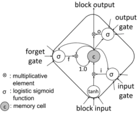
To overcome this issue, we can use LSTM blocks instead of sim-ple neurons in each hidden layer. As represented on Figure 2, each LSTM block involves a memory cell. While the network is perform-ing the classification, its content is controlled at each time step by the input and forget gates. The cell can store the input of the block it belongs to as long as necessary. The block output is controlled by the output gate. During the training phase, error signals can be trapped within a memory cell, multiplicative gates will have to learn

Fig. 2. LSTM block

which error to trap and when to release it. LSTM blocks are thus designed to solve the vanishing gradient problem [12]. The previous iterative procedure to compute the output vector of each hidden layer (equation (2)) is modified as follows [13, 14]:

i(n)t = σ(W (n−1,n) (h,i) h (n−1) t + W (n,n) (h,i)h (n) t−1 +W(n,n)_(c,i) c(n)_t−1+ b(n)_i ) (4) ft(n)= σ(W (n−1,n) (h,f ) h (n−1) t + W (n,n) (h,f )h (n) t−1 +W(n,n)_{(c,f )}c(n)t−1+ b (n) f ) (5) c(n)_t = f_t(n) c(n)t−1+ i (n) t  tanh(W (n−1,n) (h,c) h (n−1) t +W_(h,c)(n,n)h(n)_t−1+ b(n)c ) (6) o(n)t = σ(W (n−1,n) (h,o) h (n−1) t + W (n,n) (h,o)h (n) t−1 +W(n,n)_(c,o)c(n)t + b (n) o ) (7) h(n)_t = o(n)_t  tanh(c(n)t ) (8)

where  denotes the element-wise product. σ(·) and tanh(·) are re-spectively the element-wise logistic sigmoid and hyperbolic tangent functions. i(n)t , f (n) t , o (n) t and c (n)

t are respectively the input gate,

forget gate, output gate and memory cell activation vectors at hidden layer n and time frame t. These vectors are of the same size as the hidden vector h(n)t , that is the number of LSTM blocks in hidden

layer n. Hidden vectors and memory cell vectors are set to zero at t = 0. Note that equations (4) to (7) involve different weight ma-trices W(·,n)_(·,·), and bias vectors b(·)(n). Moreover, the weight

matri-ces from memory cells to multiplicative gates W(n,n)_(c,·) are diagonal, so that a multiplicative gate only considers the memory cell of the LSTM block it belongs to.

2.3. Bidirectional Recurrent Neural Networks

RNNs are only able to make use of a past temporal context. When the whole sequence of input features is available, it can be useful to exploit the future context as well. This can be done using a bidirec-tional RNN (BRNN). Each hidden layer of a BRNN contains two independent layers: the forward layer (→) that applies equation (2) from t = 1 to t = T and the backward layer (←) that proceeds in the reverse order, replacing t − 1 by t + 1 and iterating over t = T, ..., 1. For each time step t, the activations of the n-th forward and back-ward hidden layers are concatenated in a single vector (equation (9)) and supplied as an input to the next layer:

h(n)_t = [

−→

h(n)_t ;

←−

LSTM-RNNs have proven their superiority over standard RNNs to learn long-term dependencies [12] and with a precise timing [15]. To make use of a long-range past and future temporal context to clas-sify each input vector, the ideas of deep BRNNs and LSTM can thus be combined to form deep BLSTM-RNNs. This is the architecture we adopted in this study.

3. SYSTEM OVERVIEW

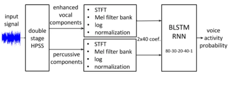
Fig. 3. System Overview

As represented on Figure 3, the proposed system first applies a double stage HPSS as pre-processing. Features are then extracted from a filter bank on a Mel scale and supplied as input to the deep BLSTM-RNN. The blocks of our system are described in more de-tails below.

3.1. Feature Extraction

Instead of presenting high-level features at the input of the classifier, whose design is essentially handcrafted and possibly sub-optimal, we chose to use low-level features, extracted from a filter bank dis-tributed on a Mel scale. We were hoping that, through the hidden layers, a deep architecture would be able to extract higher-level rep-resentations of the input data, fitted to our task.

To compute the features, we work on mono signals resampled at 16kHz and normalized to lie between −1 and 1. We first ap-ply a double stage HPSS as proposed in [16]. The original idea of HPSS [8] is to decompose the spectrogram of the input signal into one spectrogram smooth in time direction, associated to harmonic components, and another spectrogram smooth in frequency direc-tion, associated to percussive components. Singing voice is a fluc-tuating sound, not as stationary as harmonic instruments like piano or guitar, but obviously much more than percussive ones, it thus lies between harmonic and percussive components in HPSS. By control-ling the time/frequency resolution through the analysis window, we thus can consider the partials of singing voice as smooth in time or frequency direction. From a first HPSS with a long (256ms) anal-ysis window, singing voice is associated to percussive components into a signal p1(t), and separated from temporally-stable, harmonic

sounds contained in a signal h1(t). Applying a second HPSS from

p1(t), with a short analysis window (32ms), singing voice is then

associated to harmonic components into a signal h2(t), and isolated

from percussive sounds that will be contained in a signal p2(t).

Fi-nally, h2(t) is a rough estimation of the singing voice signal.

For each of the three signals h1(t), p2(t) and h2(t), we

com-puted the Short-Time Fourier Transform (STFT) with a 32ms Hann window and 50% overlap. 40 coefficients are then extracted from 40 triangular filters linearly spaced on a Mel scale with 50% over-lap. A frequency equal to f Hertz is mapped to Mel by fM el =

2595 log(1 + f /700) [17]. We tried different combinations of fea-tures from the three signals, we obtained the best results by keep-ing features from signals associated to skeep-ingkeep-ing voice and percussive

components. Our feature vector is thus 80 coefficient-long corre-sponding to the concatenation of the outputs of the filter bank ap-plied to h2(t) and p2(t). We consider the logarithm of this vector,

in order to reduce the dynamics of the data. Finally, each dimension of the input vector is normalized so as to have a mean close to zero and a standard deviation close to 1 over the training database. This conditioning, along with weights initialization, is important in order to prevent neurons saturation and to make the learning fast [18].

3.2. Building the Network by Incremental Training

bn: 10 20 30 40 50

80-b1-1 15.5 14.6 13.5 14.1 14.2

80-30-b2-1 11.4 10.7 12.2 12.4 14.0

80-30-20-b3-1 9.4 9.3 10.5 8.5 9.6

80-30-20-40-b4-1 9.3 10.0 9.4 12.0 9.4

Table 1. Classification error (%) on the Jamendo test dataset (cf. Section 4.1) according to the network architecture - The left column gives layer sizes from input to output - bnis the number of LSTM

blocks in hidden layer n.

A difficulty with neural networks is that there is no theoretical evidence to define the architecture a priori for a given task, that is the number of hidden layers and the number of neurons or LSTM blocks within each layer. The input layer size is fixed by the dimension of the input vector, 80 for our experiments. As we are working on a binary classification task, there is one unique neuron in the output layer with a logistic sigmoid activation function. Its output is an estimation of the probability of singing voice presence.

For a deep RNN with several hidden layers, an incremental cedure to train the network has been proposed in [19], which pro-gressively adds the hidden layers. It allows each layer to have some time during training in which it is directly connected to the output layer. When a hidden layer is added, the weights previously learned from the layers below are kept and then the whole network is trained. For the current hidden layer and the output one, we choose to initial-ize the weights according to a Gaussian distribution with mean 0 and standard deviation 0.1. We found this training procedure to be more effective than a raw training of the whole network. The explanation is suggested in [20], the authors experimentally show that in a super-vised gradient-trained deep neural network with random weights ini-tialization, layers far from the outputs are poorly optimized. The au-thors thus propose an independent pre-training of each hidden layer. The incremental procedure we used here is another solution.

In our work, we extended this procedure in order to automati-cally learn the network architecture during the training: we add hid-den layers progressively and for each one we choose the size bnthat

minimizes the classification error on the test dataset, as represented in Table 1. The procedure is stopped when adding a new hidden layer does not improve the classification results. When training a neural network, we are not much interested in the optimization problem, but rather in the generalization one. By considering the classifica-tion error on the test dataset, we are looking for the model that best generalizes to unseen data.

As we can see from the results in Table 1, the best architecture we found is a BLSTM-RNN with three hidden layers whose sizes are 30, 20 and 40. Within each layer, LSTM blocks are fairly distributed between forward and backward layers.

3.3. Training Algorithm

As the output of the network is an estimation of the probability of singing voice presence, we used the cross-entropy error as loss func-tion. Each training phase is done by Back-Propagation Through Time (BPTT) in the context of LSTM networks [21, 14]. We used the open-source CURRENNT Toolkit1_{which implements BPTT on}

a Graphics Processing Unit (GPU). Weights are updated after each sequence. Within each epoch, sequences are selected randomly.

Over-fitting is controlled by early-stopping: training starts with a step for the gradient descent η = 10−5and a momentum m = 0.9. If the cross-entropy error does not improve on the validation set af-ter 20 epochs, we set η = 10−6and the training continues from the weights associated with the last improvement. After 10 epochs, if there is no improvement, we set η = 10−7and the training contin-ues as before, and finally, if there is no improvement with this last step during 10 epochs, training is stopped. The momentum is cho-sen close to one in order to keep inertia high enough to avoid local minima and to attenuate the oscillatory trajectory of the stochastic gradient descent.

4. RESULTS

4.1. Jamendo : A Common Benchmark Dataset

For our experiments, we used the Jamendo Corpus, a publicly avail-able dataset including singing voice activity annotations. It contains 93 copyright-free songs, retrieved from the Jamendo website2

. The database was built and published along with [5]. The corpus is di-vided into three sets: the training set contains 61 files, the validation and test sets contain 16 songs each. This is a common database, which provides a fair comparison of our approach with others from the literature.

4.2. Network Functioning

Fig. 4. Network functioning on a 7s excerpt of ”03 - Say me good-bye” from the Jamendo test database - color scale between -1 (white) and +1 (black) - ”Output” belongs to [0,1] - ”Decision” and ”Truth” belong to {0,1} in which 0 (grey segments) denotes voice absence and 1 (black segments) denotes voice presence.

1_{http://sourceforge.net/p/currennt} 2_{http://www.jamendo.com}

To highlight the network internal functioning, we represent on Figure 4 the sequence of input vectors (h2(t) at the lower half and

p2(t) at the upper one, cf. Section 3.1), the output of each hidden

layer, the output of the network which is an estimation of the prob-ability of singing voice presence, the decision taken by the network by thresholding this probability at 0.5, and the ground truth for about 7s of a track from the Jamendo test dataset. Through the depth of the network, the outputs of the layers are more and more stable and a clear temporal structure emerges, with the appearance of segments associated to singing voice presence/absence. From a low-level rep-resentation, which is highly temporally variable, extracted by a filter bank on a Mel scale, the network is able to extract a simple repre-sentation at the output of the third hidden layer, highlighting singing voice presence. The track we used here contains a long total silence section. We can see that the outputs of the hidden layers continue to vary during this section while inputs remain constant. This observa-tion shows that the network has learned a temporal context. 4.3. Results

To evaluate the performance of our system, we compute four com-mon evaluation measures [22] considering all the frames of the test set. The classification Accuracy is the proportion of frames correctly classified. The Recall is the proportion of frames labeled as voiced in the ground truth that are estimated as voiced by the algorithm. The Precision is the proportion of frames estimated as voiced by the algorithm that are effectively voiced in the ground truth. Finally, the F-measure(also called F1 score) is a global performance measure corresponding to the harmonic mean of precision and recall.

Table 2 compares the results of our method with those from [5], [6] and [7], the latter being the one which provided the best results on this database to the best of our knowledge. We see that over all the measures, our system performs better. This is remarkable consid-ering that we used simple low-level features and no post-processing. In [7], Lehner et al. improved precision by means of specifically de-signed features but to the detriment of recall compared to their pre-vious method in [6]. In fact, manually designing high-level features can be sub-optimal. Conversely, the deep BLSTM-RNN we used has automatically learned how to extract useful information from low-level features to finally improve both recall and precision. This is noticeable and explains the particularly high F-measure we obtain.

RAMONA [5] LEHNER(a) [6] LEHNER(b) [7] NEW Accuracy (%) 82.2 84.8 88.2 91.5

Recall (%) n/a 90.4 86.2 92.6 Precision (%) n/a 79.5 88.0 89.5 F-measure 84.3 84.6 87.1 91.0

Table 2. Singing voice detection results on Jamendo test database 5. CONCLUSION

In this paper we presented a new approach for singing voice detec-tion. Instead of working on defining a complex feature set, we took advantage of neural networks to extract simple representations fitted to our task from low-level features. Furthermore, the BLSTM-RNN we used is a classifier that inherently takes a temporal context into account, thus discarding the necessity of post-processing to handle sequential aspects. This new method significantly improved state-of-the-art results on a common database. This performance encourages further work with BLSTM-RNN in music information retrieval for sequence classification tasks, for instance in the context of automatic melody estimation.

6. REFERENCES

[1] Justin Salamon, Emilia Gomez, Dan Ellis, and Ga¨el Richard, “Melody extraction from polyphonic music signals: Ap-proaches, applications and challenges,” IEEE Signal Process-ing magazine, vol. 31, no. 2, pp. 118–134, Mar. 2014. [2] Chao-Ling Hsu, DeLiang Wang, Jyh-Shing Roger Jang, and

Ke Hu, “A tandem algorithm for singing pitch extraction and voice separation from music accompaniment,” IEEE Transac-tions on Audio, Speech, and Language Processing, vol. 20, no. 5, pp. 1482–1491, Jul. 2012.

[3] Shankar Vembu and Stephan Baumann, “Separation of vocals from polyphonic audio recordings,” in International Society for Music Information Retrieval (ISMIR) Conference, London, UK, Sep. 2005, pp. 337–344.

[4] Youngmoo E. Kim and Brian Whitman, “Singer identification in popular music recordings using voice coding features,” in International Society for Music Information Retrieval (ISMIR) Conference, Paris, France, Oct. 2002, vol. 13, p. 17.

[5] Mathieu Ramona, Ga¨el Richard, and Bertrand David, “Vocal detection in music with support vector machines,” in IEEE In-ternational Conference on Acoustics, Speech and Signal Pro-cessing (ICASSP), Las Vegas, Nevada, USA, Mar. - Apr. 2008, pp. 1885–1888.

[6] Bernhard Lehner, Reinhard Sonnleitner, and Gerhard Widmer, “Towards light-weight, real-time-capable singing voice detec-tion.,” in International Society for Music Information Retrieval (ISMIR) Conference, Curitiba, Brazil, Nov. 2013, pp. 53–58. [7] Bernhard Lehner, Gerhard Widmer, and Reinhard Sonnleitner,

“On the reduction of false positives in singing voice detection,” in IEEE International Conference on Acoustics, Speech and Signal Processing (ICASSP), Florence, Italy, May 2014, pp. 7480–7484.

[8] Nobutaka Ono, Kenichi Miyamoto, Jonathan Le Roux, Hi-rokazu Kameoka, and Shigeki Sagayama, “Separation of a monaural audio signal into harmonic/percussive compo-nents by complementary diffusion on spectrogram,” in Eu-ropean Signal Processing Conference (EUSIPCO), Lausanne, Switzerland, Aug. 2008.

[9] Mart´ın Rocamora and Perfecto Herrera, “Comparing audio de-scriptors for singing voice detection in music audio files,” in Brazilian Symposium on Computer Music (SBCM), San Pablo, Brazil, Sep. 2007, vol. 26, p. 27.

[10] Lise Regnier and Geoffroy Peeters, “Singing voice detection in music tracks using direct voice vibrato detection,” in IEEE International Conference on Acoustics, Speech and Signal Pro-cessing (ICASSP), Taipei,Taiwan, Apr. 2009, pp. 1685–1688. [11] Sepp Hochreiter, Yoshua Bengio, Paolo Frasconi, and J¨urgen

Schmidhuber, “Gradient flow in recurrent nets: the difficulty of learning long-term dependencies,” in A Field Guide to Dy-namical Recurrent Neural Networks, Kremer and Kolen, Eds. IEEE Press, 2001.

[12] Sepp Hochreiter and J¨urgen Schmidhuber, “Long short-term memory,” Neural computation, vol. 9, no. 8, pp. 1735–1780, Nov. 1997.

[13] Alex Graves, Abdel-rahman Mohamed, and Geoffrey Hinton, “Speech recognition with deep recurrent neural networks,” in

IEEE International Conference on Acoustics, Speech and Sig-nal Processing (ICASSP), Vancouver, BC, Canada, May 2013, pp. 6645–6649.

[14] Alex Graves, Supervised Sequence Labelling with Recur-rent Neural Networks, Ph.D. thesis, Technische Universit¨at M¨unchen, Jul. 2008.

[15] Felix A. Gers, Nicol N. Schraudolph, and J¨urgen Schmidhuber, “Learning precise timing with LSTM recurrent networks,” The Journal of Machine Learning Research, vol. 3, pp. 115–143, Aug. 2002.

[16] Hideyuki Tachibana, Takuma Ono, Nobutaka Ono, and Shigeki Sagayama, “Melody line estimation in homophonic music au-dio signals based on temporal-variability of melodic source,” in IEEE International Conference on Acoustics, Speech and Signal Processing (ICASSP), Dallas, Texas, USA, Mar. 2010, pp. 425–428.

[17] Douglas D. O’Shaughnessy, Speech communications - human and machine (2. ed.)., IEEE Press, 2000, p. 128.

[18] Yann LeCun, Leon Bottou, Genevieve B. Orr, and Klaus-Robert M¨uller, “Efficient BackProp,” in Neural Networks: Tricks of the trade, Genevieve B. Orr and Klaus-Robert M¨uller, Eds. 1998, Springer.

[19] Michiel Hermans and Benjamin Schrauwen, “Training and analysing deep recurrent neural networks,” in Advances in Neural Information Processing Systems (NIPS), Harrahs and Harveys, Lake Tahoe, Nevada, United States, Dec. 2013, pp. 190–198.

[20] Yoshua Bengio, Pascal Lamblin, Dan Popovici, and Hugo Larochelle, “Greedy layer-wise training of deep networks,” in Advances in Neural Information Processing Systems (NIPS), Vancouver, BC, Canada, Dec. 2007, vol. 19, p. 153.

[21] Alex Graves and J¨urgen Schmidhuber, “Framewise phoneme classification with bidirectional LSTM and other neural net-work architectures,” Neural Netnet-works, Jul.-Aug. 2005. [22] Marina Sokolova and Guy Lapalme, “A systematic analysis

of performance measures for classification tasks,” Information Processing & Management, vol. 45, no. 4, pp. 427–437, Jul. 2009.