HAL Id: hal-01219088
https://hal.archives-ouvertes.fr/hal-01219088
Submitted on 22 Oct 2015
HAL is a multi-disciplinary open access
archive for the deposit and dissemination of sci-entific research documents, whether they are pub-lished or not. The documents may come from teaching and research institutions in France or
L’archive ouverte pluridisciplinaire HAL, est destinée au dépôt et à la diffusion de documents scientifiques de niveau recherche, publiés ou non, émanant des établissements d’enseignement et de recherche français ou étrangers, des laboratoires
A characterization of quasi-rational polygons
Nicolas Bedaride
To cite this version:
Nicolas Bedaride. A characterization of quasi-rational polygons. Nonlinearity, IOP Publishing, 2012, �10.1088/0951-7715/25/11/3099�. �hal-01219088�
A characterization of quasi-rational polygons
Nicolas Bedaride∗ September 10, 2012
ABSTRACT
The aim of this paper is to study quasi-rational polygons related to the outer billiard. We compare different notions introduced in [GS92] and [Sch09] and make a synthesis of those.
1
Introduction
The outer billiard map is a transformation T of the exterior of a planar convex bounded domain D defined as follows: T (M ) = N if the segment M N is tangent to the boundary of D at its midpoint, and D lies at the right of M N . The outer billiard map is not defined if the tangent segment M N shares more than one point with the boundary of D. In the case where P is a convex polygon; the set of points for which T or any of its iterations is not defined is contained in a countable union of lines and has zero measure. The dual billiard map has been introduced by Neumann in [Neu59] as a toy model for the planet orbits. One of the most interesting questions was whether the orbits of T might escape to infinity for a polygonal domain D. Two particular classes of polygons have been introduced by Kolodziej et al. in several articles, see [Ko l89, GS92, VS87]. These classes are named rational and quasi-rational polygons and contain all the regular polygons. A rational polygon has vertices on a lattice of R2. They prove that every orbit outside a polygon in this class is bounded. Every regular polygon is a quasi-rational polygon, and it is not a rational polygon except if there are 3, 4 or 6 edges. In the case of the regular pentagon, Tabachnikov completely described the dynamics of the outer billiard map in terms of symbolic dy-namics, see [Tab95b]. He proves that some orbits are bounded and non periodic. The symbolic coding of this map has been given in [BC11] for a regular polygon with 3, 4, 5, 6 and 10 edges.
For non quasi-rational polygons, there is no general study. The case of trapezoids has been studied. The set of trapezoids can be parametrized up
∗
Laboratoire d’Analyse Topologie et Probabilit´es UMR 7353, Universit´e Aix Marseille, avenue escadrille Normandie Niemen 13397 Marseille cedex 20, France. [email protected]
to affinity by one parameter. For an irrational parameter, it is not a quasi-rational polygon, and the proof of [GS92] cannot be used for a polygon with parallel sides. Nevertheless, Li proved that all the orbits of the outer billiard map are bounded (this theorem is also proved by Genin) see [Li09] and [Gen08]. Recently Schwartz described a family of quadrilaterals, named kites, for which there exists unbounded orbits, see [Sch07] and [Sch09]. In these papers Schwartz introduces many tools in order to study the dynamics. These tools can also be used in the case of regular polygons, see [Sch10].
In this article we investigate the case of quasi-rational polygons. The main achievements of the paper consist of a synthesis of results of [GS92] and the notions introduced by Schwartz. These links allow us to give a new characterization of this class and to give some simple conditions which guarantee the quasi rationality.
Remark 1. In this article, P is a polygon with n vertices without parallel edges, see last section for some comments. All the figures correspond to the same polygon.
2
Overview of the paper
First we recall usual definitions about dual billiard in Section 3 and introduce our definition of quasi-rational polygon. Next, in Section 5, we show that our definition is equivalent to the old one of [GS92] and also similar to [Sch09]. In Section 6 we prove the classical theorem on quasi-rational polygon using our definition. Finally in Section 8 we use our definition to obtain new results on quasi-rational polygons.
Acknowledgment: This work has been supported by the Agence Nationale de la Recherche – ANR-10-JCJC 01010.
3
Outer billiard
We refer to [Tab95a] or [GS92]. We consider a convex polygon P in R2 with n vertices. Let P = R2\ P be the complement of P .
We fix an orientation on R2. We will define the outer billiard map off a countable union of lines. The map will be defined for all time.
For a point M ∈ P , there are two half-lines R, R0 emanating from M and tangent to P , see Figure 1. Assume that the oriented angle R, R0 has positive measure. Denote by A+, A− the tangent points on R respectively R0. We say that A+ is the vertex associated to M .
Definition 1. The outer billiard map is the map T defined as follows: T (M ) = rA+(M )
• T M • M A+ A− • T−1M R
Figure 1: The outer billiard map
Definition 2. A polygon P is said to be rational if the vertices of P are on a lattice of R2.
We refer to [Sch09]. Consider a polygon without parallel edges. Assume the edges are oriented counterclockwise sense (while T is oriented clockwise). For each edge, consider the vertex of P furthest from the line supporting the edge. It is unique by convexity and assumption. Then denote by V the vector equal to twice the vector between the final vertex of the edge and this vertex. A strip is the band formed by the line supporting the edge and V , see Figure 2. It is denoted (Σ, V ) or Σ if clear from the context. We index them with respect to the slopes of the sides of the polygon, this gives the sequences (Σi, Vi)1≤i≤n.
Definition 3. Let α1, . . . , αnbe non zero real numbers, we say that (α1, . . . , αn)
are commensurate if α2
α1, . . . ,
αn
αn−1 are rational numbers.
We denote by u ∧ v the cross product of two vectors u, v of the plane. It is a vector of R3 orthogonal to the plane with only one non zero coordinate. The absolute value of this coordinate is denoted |u ∧ v|.
Definition 4. The polygon P is quasi-rational if and only if (|V1∧ V2|, . . . , |Vn∧ V1|) are commensurates.
For example, consider the polygon with vertices A, B, C, D, see Figure 2. The vectors are equal to: V1 = 2 ~CB, V2 = 2 ~AC, V3 = 2 ~BD, V4= 2 ~BA.
4
Unfolding
In this Section we recall the notion of unfolding introduced in [GS92]. This notion is used to transform the outer billiard map in a piecewise translation map defined on cones.
C
A B
D
Figure 2: Polygon and strips
4.1 Definitions
Consider two vertices A, B of P , and the images of P by the rotations rA, rB of angle π. They are equal up to translation. Denote by ˜P one of
these polygons. Let SP be the set of those polygons in R2 that are images
by a translation by P or ˜P . Let M be a point in P , define the following bijective map.
πM : SP → R2× {−1, 1}
Q 7→ (A, ε)
Consider the image of M by the outer billiard map outside Q. It is obtained by a rotation of angle π centered at a vertex of Q. Let A be this vertex of Q. Moreover we take ε = 1 if Q is a translate of P , ε = −1 if Q is a translate of ˜P . We say A is associated to M for Q. It is clear that πM is
a bijection.
We define a new map called the unfolding of the dual billiard map. ˜
T : R2× {−1, 1} → R2× {−1, 1} (A, ε) 7→ (A0, −ε)
The ordered pair (A, ε) comes from a polygon Q via the map πM. Consider
the polygon Q0 image of the polygon Q by a rotation of angle π of center A, see Figure 3. The point A0 is the vertex associated to M for Q0.
l1 M l3 A0 A M
Figure 3: Necklace dynamics
The dynamics of this map is related to the outer billiard map by the following result. In what follows we will also denote by ˜T the projection of
˜ T to R2.
Definition 5. Denote by (li)i≤n the lines passing through M and parallel
to the edges of P . They defines 2n cones (Ci)1≤i≤2n. The boundary of each
cone is made of two half lines denoted Ri, Ri+1.
Proposition 1. [GS92] We have: • The sequence (Tk(M ))
kis bounded (resp. periodic) if and only if there
exists a point Q ∈ R2× {−1, 1} such that the orbit of Q is bounded (resp. periodic) for ˜T .
• For every cone Ci, there exists a vector ai such that if A, ˜T A ∈ Ci, then
the restriction of ˜T to a cone is a translation of vector ai. Moreover
we have for every integer i, an+i= −ai.
• There exists a polygon P∗ with 2n edges, with vertices on C1, . . . , Cn
such that each side is parallel to some ai.
The sides of P∗ will be denoted vi∗, i = 1 . . . 2n.
4.2 Some results
Here we explain how to find the vectors a1, . . . , an.
Definition 6. For each cone Ci, let di be a vector parallel to the edge li
such that di+ ai is colinear to li+1.
Proposition 2. Consider the cone bounded by the lines li, li+1 and
associ-ated to the vector ai. We have
• The strips associated to the lines li and li+1 are consecutive for the
l1
M l3
Figure 4: Polygon P∗ associated to the quadrilateral ABCD
• The vectors ai, ai+1 have one vertex in common.
• The parallelogramm Σi∩ Σi+1 has ai for diagonal and di for one side.
The area of Σi∩ Σi+1 is equal to |ai∧ di|.
Proof. Consider the cone Ci with boundaries li, li+1 and a polygon Q ∈ SP.
Let A be the vertex of Q associated to M . The first thing to remark is that the slope of the line (AM ) is between the slopes of li and li+1. Thus
A belongs to the edge parallel to li+1and the point ˜T A belongs to the edge
parallel to li. This proves Vi = ai and the first point.
Consider one strip with vertices A, B, M , it means that M is the vertex that maximized the distance from (AB). By definition the polygon is in the strip between (AB) and M + R ~AB. Let N be the vertex neighbour of M in the polygon. Assume the vertex associated to (M N ) is not B, denote it B0. The polygon is in the strip associated to M, N, B0. Thus this strip does not intersect the segment [AB]. Then the line (M N ) has a slope bigger than (BB0). First part implies that in the ordering of the slopes, the slope of (M N ) is the consecutive of the slope of (AB), contradiction.
The vector di is on the boundary of Σi by definition. Denote ai= v − w
with v, w vertices of P . By the previous point, there exists a vertex w0 such that ww0 is on the boundary of Σi+1. Thus one side of Σi∩ Σi+1is given by
the line ww0 and one side by the line di. The area of the parallelogramm is
the cross product of one side by the diagonal.
4.3 Comments
The preceding proposition may seem awkward, since we are not studying directly the outer billiard map to obtain results on its dynamics. Never-theless we can transform the statement in terms of the outer billiard map T . The map T2 is a piecewise translation, defined on several subsets of R2.
C A B D 2 ~BA 2 ~BD 2 ~BC 2 ~AC 2 ~AB 2 ~DB 2 ~CB 2 ~CA Figure 5: Definition of T2
Some of them can be compact sets, see Figure 5. Outside a compact region containing the polygon, the sets are unbounded and the translation vectors are two by two opposite. The translation vectors are exactly the vectors Vi, see Proposition 2. The dynamics of T2 is simple: A point m begins its
trajectory by being translated by a vector Vi until it reaches another set
where it moves by another vector Vi. Thus an orbit of point far away from
P looks like the polygon P∗. The link between T2 and the piecewise trans-lations of vectors V1. . . Vn can be extended to a neighborhood of P , but it
is much more complicated, see the Pinwheel theorem [Sch11]. It is related in Proposition 1 to the case where A is closed to M . It is possible that the condition A, ˜T A ∈ Ci is not verified. This case is treated by the Pinwheel
theorem in [Sch09].
5
Equivalence
5.1 Statement of results
The aim is to prove
Theorem 1. The followings are equivalent: • (v1∗
|a1|, . . . ,
v∗n
|an|) are in PQ
n.
• (|a1∧ a2|, . . . , |an∧ a1|) are commensurates.
Remark 2. The first point is the initial definition of a quasi-rational polygon given in [GS92]. The third is the definition by Schwartz in [Sch09].
To do this we will prove the three following propositions. The theorem will be a clear consequence with help of Proposition 2.
Proposition 3. The following are equivalent: • There exists a rational solution (t1, . . . , tn) to
d1+ a1 = t2d2 d1+ a1+ t2a2= t3d3 d1+ a1+ . . . tnan= −d1
• (|a1∧ d1|, . . . , |an∧ dn|) are commensurates.
Proposition 4. The following are equivalent: • There exists a rational solution (t1, . . . , tn) to
d1+ a1 = t2d2 d1+ a1+ t2a2= t3d3 d1+ a1+ . . . tnan= −d1 • P is a quasi-rational polygon.
Proposition 5. The following are equivalent: • There exists a rational solution (t1, . . . , tn) to
d1+ a1 = t2d2 d1+ a1+ t2a2= t3d3 d1+ a1+ . . . tnan= −d1 • (v1∗ |a1|, . . . , v∗n |an|) are in PQ n. 5.2 Proof of Proposition 3
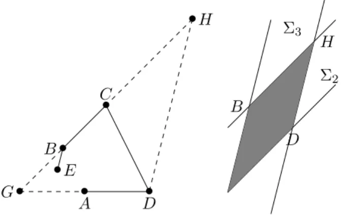
The proof is based on Figure 6. Consider a polygon such that the points A, B, C, D, E are vertices labelled in such a way that the slopes of edges are in the increasing order AD, BC, BE. Also assume we have a1 = 2 ~DC.
Then Proposition 2 implies that a2 = 2 ~BD. Let G be the intersection point
of (AD) and (BC), and let H a point on the line (BC) such that (HD) is parallel to (BE). Then we have d1 = 2 ~GD, d2 = 2 ~HB. Moreover Σ1∩ Σ2 is
• A D• • B • C • G • H • E D B H Σ3 Σ2
Figure 6: Proof of Proposition 3
real number such that ~BH = r ~GC. We see that Σ1is given by ((AD), 2 ~DC),
Σ2 = ((BC), 2 ~BD). The intersection of the two strips Σ1, Σ2 has DC as a
diagonal. A similar computation gives the intersection of the strips Σ3, Σ2.
The two parallelograms are constructed on triangles BHD, GCD. We have |BHD| = | ~BH ∧ ~BD|
|GCD| = | ~GC ∧ ~CD| = | ~GC ∧ ~BD| = r|BHD|.
The ratio of the areas of the two parallelograms is the same as the ratio of the area of triangles, thus it is equal to r. Thus we have proved:
r ∈ Q ⇐⇒ |Σ|Σ1∩ Σ2|
2∩ Σ3| ∈ Q.
Note that r is equal to the inverse of t2 in the first part of Proposition. The
proof of Proposition follows by induction.
5.3 Proof of Proposition 4
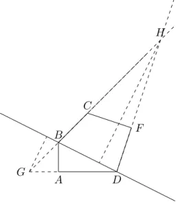
The proof is based on Figure 7. Consider an edge AD, and the associated vector a1 = 2 ~DC. By Proposition 2 the vector a2 is equal to 2 ~BD with
BC edge of the polygon, and a3 = 2 ~F B, with DF edge of the polygon.
Let us call G the intersection of (CB) with (AD), and H the intersection of (CB) and (DF ). Then d1 = 2 ~GD, d2 = 2 ~HB. Assume that the first
item of Proposition 4 holds. Then there exist r, r0 ∈ Q such that ~GC = r ~HB, ~HD = r0DF . Solving system shows that d~ i is a rational linear sum
of a1, . . . , an. By Proposition 2, the edges of P are rational combination of
a1, . . . , an, the assumption implies: ~GC = q ~BC, ~HD = q0F D with q, q~ 0 ∈ Q.
Now the relations ~GC = q ~BC = r ~HB imply ~HB = q” ~CB with q00 rational number. For a point M , denote hM the length of the orthogonal projection
of M on (DB). The relations HB = q” ~~ CB, ~HD = q ~F D gives hH = q”hC
and hF = qhH. By Proposition 2, the areas |a1∧ a2|, |a2∧ a3| are given by
areas of triangles BCD, DBF . The ratio of these areas is equal to the ratio between hC and hF. Thus the areas are commensurates. The other part of
the proof is similar.
A D B C G H F
Figure 7: Proof of Proposition 4
5.4 Proof of Proposition 5
The proof is based on Figure 4. By Proposition 4 we know that the first statement is equivalent to the fact that P is a quasi-rational polygon. If the system has a rational solution, then the polygon defined by d1, d1 +
a1, . . . , d1 + a1+ . . . tnan is some polygon P∗. The edges v1∗, . . . , vn∗ of this
polygon are equal to a1, t2a2, . . . , tnan, thus the first implication is proved.
Conversly, consider the point M on l1 such thatOM = d~ 1. By
hypoth-esis, there exists a polygon with sides r1a1, . . . rnan with rational numbers
ri, i ≤ n. Thus there exists an homothetic image of this polygon with vertex
M , and all the edges fulfilling the same condition. This gives a rational solution of the system.
This proposition can be reformulated in
rational numbers t2, . . . , tn and M ∈ R2 such that M ∈ l1 M + a1 ∈ l2 M + a1+ t2a2∈ l2 M + a1+ · · · + tiai∈ li M + a1+ · · · + tnan= −M
6
All orbits are bounded for quasi-rational
poly-gons
In this section we give a new proof of the following theorem using our defini-tion of quasi-radefini-tional polygon. The aim is to understand the general outline of the proof, not to explain all the details.
Theorem 2. [GS92] For a quasi-rational polygon, every orbit of the dual billiard map is bounded.
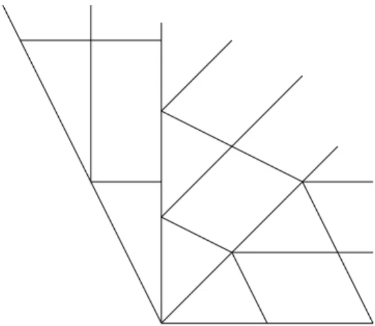
We consider the unfolding and the cone C1. We can tile periodically this
cone by a parallelogramm with one side equal to d1 and one diagonal equal
to a1. The same thing can be done in all cones. Consider a point x and the
first hitting map with the next cone: f1. We have f1(x+d1) = f1(x)+a1+d1,
we deduce f2(f1(x + d1)) = f2(f1(x) + t2d2). Since the polygon is
quasi-rational there exists an integer n such that f2(f1(x + nd1)) = f2(f1(x) +
nt2d2) = f2(x) + n0(a2+ d2). Now the first return map to the cone C1 is the
composition of f1, . . . , fn. We obtain that there exists a vector u such that
for every x
F (x + u) = F (x) + u
In term of parallelograms, it means that we consider a point in one box and take the image of the box by F . We have a second periodic tiling of the cone by a parallelogram with side u and diagonal a1. The orbit of the point
x depends on the cutting of a box of the new tiling by the initial one. If the two tilings are commensurates then every orbit is bounded. We must compare u and d1: they are rationally proportional by definition of
quasi-rational polygon. If P is quasi-rational every box is mapped by F to a box, thus every orbit is periodic.
7
Graph of spokes
7.1 Definitions
By definition, for each integer i, aiis a vector between two vertices of P , and
Figure 8: Tilings of consecutive cones
vertices of P , and there is an oriented edge starting from each vertex and joining the end of the vector ai associated to the vertex. Denote it S(P ),
and we call it the graph of spokes.
Example 1. Consider the polygon ABCD of Figure 1, then S(P ) is given by B C ~~ A //D OO
Figure 9: Graph of spokes
Lemma 1. This graph has following properties: • Each vertex has an outgoing edge.
• Two edges can not have the same vertices. • The graph contains a cycle.
Proof. Proof left to the reader for the two first items. An edge between vertices A, B implies that some vector ai = AB. Thus the graph is the~
same thing as a map defined on the set of vertices. This map is defined everywhere but not necessarily injective. It is injective on a subset. On this subset the graph is a cycle.
Corollary 2. For every polygon, there exists a rational relation between the vectors a1, . . . , an.
Proof. By preceding Lemma there exists a cycle in the graph. It implies that the sum of vectors ai associated to this cycle is null.
Remark 3. The notion of spokes is used in outer billiard by Schwartz to prove its result on the pinwheel map, see [Sch10].
We now use the preceding tools to obtain new results on quasi-rational polygons.
8
Description of quasi-rational polygons
Theorem 3. We have:
• A quadrilateral is a quasi-rational polygon if and only if it is rational. • There exists a non regular and non rational quasi-rational pentagon. • Assume the graph of spokes is a cycle (or an union of cycles). Then
the polygon is quasi-rational.
Proof. • Consider (a1, a2) as a basis of R2, denote α, β the coordinates of
a3 in this basis, and (γ, δ) those of a4: a3 = αa1+ βa2, a4 = γa1+ δa2.
The numbers |a1∧ a2|, |a3∧ a2|, |a4∧ a3|, |a4∧ a1| are proportional to
1, α, αδ − βγ, δ. If the polygon is quasi-rational, by Theorem 1 we deduce α, δ, αδ − βγ ∈ Q. This implies βγ ∈ Q. Now Corollary 2 implies that there exists a rational linear relation between a1, . . . , a4.
This relation concerns at least three vectors. All possibilities imply β, γ ∈ Q. Thus the polygon has vertices on a lattice.
• Consider four points on a lattice of R2. Denote these points A, B, C, E.
We will contruct a point D such that the pentagon ABCDE will be as required. It suffices to consider one point D outside the lattice. We can always choose D such that the spokes of the pentagon ABCDE are associated to vectors AC, ~~ BE, ~CE, ~DB, ~EA. Then the rational relation is a1+ a3 + a5 = 0. There is no other rational relation by
definition of D. Now we can express the vectors a1, . . . , a5 in the basis
(a1, a2). By construction a3, a5 have rational coordinates. Then we
can always choose D such that the area |a2 ∧ a3| is rational. The
constructed pentagon is quasi-rational.
• Now assume that the graph of spokes is an union of cycles. By Corol-lary 1 a polygon is quasi-rational if for every side li, there exists λ ∈ R
and rational numbers r1, . . . , rn∈ Q∗ such that
If the graph is a union of cycles, then the map defined on vertices associated to the graph of spokes is invertible. It means that each vertex is a linear combination of a1. . . an. Thus the side li can be
expressed as rational combination of the ai’s. Thus P is quasi-rational
if there exists r1. . . rn∈ Q and λ ∈ R such that:
λXr0jaj+ r1a1+ · · · + rnan= 0.
Since the graph is a cycle, there exists a rational relation between a1. . . an. Thus we can solve the equation and find r1. . . rn, r01. . . r0n.
Remark 4. Consider the example of graph in Figure 9. In this case the preceding map is not a bijection since no edge goes to B.
For regular polygon with odd number of sides (greater than five), the graph is not simply connected.
9
Remarks
9.1 Polygon with parallel sides
If the polygon has parallel sides, then the definition of [GS92] still works. Nevertheless the number of cones decreases. For the definition of [Sch09] we need to be more precise to define a strip. In this case two consecutive strips can have an intersection with infinite area. Thus the new definition of quasi-rational is that, up to a factor, the areas of Σi∩ Σi+1 are in Z ∪ {∞}
for every integer i.
9.2 Regular polygons
A regular polygon with n edges is invariant by rotation of angle 2π/n. Let ω be a n th root of unity, we have ai = ωai−1+ ai−2for every integer i. Thus
it is clear that |ai∧ ai+1| is a constant number, and a regular polygon is a
quasi-rational polygon. Moreover the graph of spokes is a cycle, since the spoke ai+1is the image of ai by rotation of angle 2π/n. This gives another
proof of previous fact.
The study of regular polygons has been done if the number of sides is equal to 5 by Tabachnikov, see [Tab95b]. A description of the symbolic dynamics has been made for regular polygons with 3, 4, 5, 6, 10 edges in [BC11]. In [Sch10] Schwartz initiates a study of the regular octogon.
References
[BC11] N. Bedaride and J. Cassaigne. Outer billiards outside regular poly-gons. Journal of London Mathematical Society, 2(83):301–323, 2011.
[Gen08] D. Genin. Research announcement: boundedness of orbits for trapezoidal outer billiards. Electron. Res. Announc. Math. Sci., 15:71–78, 2008.
[GS92] E. Gutkin and N. Sim´anyi. Dual polygonal billiards and necklace dynamics. Comm. Math. Phys., 143(3):431–449, 1992.
[Ko l89] R. Ko lodziej. The antibilliard outside a polygon. Bull. Polish Acad. Sci. Math., 37(1-6):163–168 (1990), 1989.
[Li09] L. Li. On Moser’s boundedness problem of dual billiards. Ergodic Theory Dynam. Systems, 29(2):613–635, 2009.
[Neu59] B.H.R. Neumann. Sharing ham and eggs. Iota, Manchester uni-versity Mathematics students journal, 1959.
[Sch07] R. E. Schwartz. Unbounded orbits for outer billiards. I. J. Mod. Dyn., 1(3):371–424, 2007.
[Sch09] R. E. Schwartz. Outer billiards on kites, volume 171 of Annals of Mathematics Studies. Princeton University Press, Princeton, NJ, 2009.
[Sch10] R. E. Schwartz. Outer billiards, the arithmetic graph and the octagon. Arxiv, 2010.
[Sch11] Richard Evan Schwartz. Outer billiards and the pinwheel map. J. Mod. Dyn., 5(2):255–283, 2011.
[Tab95a] S. Tabachnikov. Billiards. Panoramas et Synth`eses, 1995.
[Tab95b] S. Tabachnikov. On the dual billiard problem. Adv. Math., 115(2):221–249, 1995.
[VS87] F. Vivaldi and A. V. Shaidenko. Global stability of a class of discontinuous dual billiards. Comm. Math. Phys., 110(4):625–640, 1987.