HAL Id: halshs-01281940
https://halshs.archives-ouvertes.fr/halshs-01281940
Submitted on 3 Mar 2016
HAL is a multi-disciplinary open access
archive for the deposit and dissemination of sci-entific research documents, whether they are pub-lished or not. The documents may come from
L’archive ouverte pluridisciplinaire HAL, est destinée au dépôt et à la diffusion de documents scientifiques de niveau recherche, publiés ou non, émanant des établissements d’enseignement et de
More Accurate Measurement for Enhanced Controls:
VaR vs ES?
Dominique Guegan, Bertrand Hassani
To cite this version:
Dominique Guegan, Bertrand Hassani. More Accurate Measurement for Enhanced Controls: VaR vs ES?. 2016. �halshs-01281940�
Documents de Travail du
Centre d’Economie de la Sorbonne
More Accurate Measurement for Enhanced Controls:
VaR vs ES?
Dominique G
UEGAN,Bertrand H
ASSANIMore Accurate Measurement for Enhanced Controls: VaR vs ES?
February 13, 2016
DOMINIQUE GUEGAN1, BERTRAND K. HASSANI2.
Abstract
This paper3analyses how risks are measured in financial institutions, for instance Market, Credit, Operational, etc with respect to the choice of the risk measures, the choice of the dis-tributions used to model them and the level of confidence selected. We discuss and illustrate the characteristics, the paradoxes and the issues observed comparing the Value-at-Risk and the Expected Shortfall in practice. This paper is built as a differential diagnosis and aims at discussing the reliability of the risk measures as long as making some recommendations4.
Key words: Risk measures - Marginal distributions - Level of confidence - Capital re-quirement.
1Université Paris 1 Panthéon-Sorbonne, CES UMR 8174, 106 boulevard de l’Hopital 75647 Paris Cedex 13,
France, phone: +33144078298, e-mail: [email protected], Labex Refi
2
Grupo Santander and Université Paris 1 Panthéon-Sorbonne CES UMR 8174, 106 boulevard de l’Hopital 75647 Paris Cedex 13, France, phone: +44 (0)2070860973, e-mail: [email protected]., Labex Refi. Disclaimer: The opinions, ideas and approaches expressed or presented are those of the authors and do not necessarily reflect Santander’s position. As a result, Santander cannot be held responsible for them.
3
This work was achieved through the Laboratory of Excellence on Financial Regulation (Labex ReFi) supported by PRES heSam under the reference ANR-10-LABEX-0095
4This paper has been written in a very particular period of time as most regulatory papers written in the past
20 years are currently being questioned by both practitioners and regulators themselves. Some distress or disarray has been observed among risk managers as most models required by the regulation were not consistent with their own objective of risk management. The enlightenment brought by this paper is based on an academic analysis of the issues engendered by some pieces of regulation and it has not for purpose to create any sort of polemic.
1
Introduction
How to ensure that financial regulation allows banks to properly support the real economy and simultaneously control their risks? In this paper5 another way to look at regulatory rules is proposed, not only based on the objective to provide a capital requirement sufficiently large to protect the banks but to improve the risk controls. In this paper we offer an holistic analy-sis of risk measurement, taking into account the choice of risk measure, the distribution used and the confidence level considered simultaneously. This leads us to propose fairer and more effective solutions than regulatory proposals since 1995. Several issues are discussed: (i) the choice of the distributions to model the risks: uni-modal or multi-modal distributions; (ii) the choice of the risk measure, moving from the VaR to spectral measures. The ideas developed in this paper are relying on the fact that the existence of an adequate internal model inside banks will always be better than the application of a rigid rule preventing banks from doing the job which consists in having a good knowledge of their risks and a good strategy to control them. Indeed, in that latter case, banks have to think (i) about several scenarii to assess the risks (various forward looking information sets), and (ii) at the same time to the importance of unknown new shocks in the future to stress their internal modellings. This also imply that the regulatory capital can change over time, introducing dynamics in the computations of risk measures based on "true" information: this approach is definitely not considered by regulators but would lead to interesting discussions between risk practitioners and supervisors. Indeed, this idea would bring then closer to the real world permitting banks to play their role in funding the economy. In our argumentation, the key point remains the choice of the data sets to use, as soon as the theoretical tools are properly handled. Our purpose is illustrated using data representative of operational and market risks. Operational risks are particularly interesting for this exercise as materialised losses are usually the largest within banks, nevertheless all the tools and concepts developed in this paper are scalable and applicable to any other class of risks. We also show the importance of the choice of the period with which we work in the risk measurement.
The paper is organised as follows: in Section two we introduce and discuss a new holistic approach in terms of risks. Section three is dedicated to an exercise to illustrate our proposal providing 5This paper has been presented at Riskdata Paris (Septembre 2015), at Tianjin University (September 2015),
some recommandations to risk managers and regulators.
2
Alternative strategies for measuring the risks in financial
in-stitutions
It is compulsory for each department of a bank to evaluate the risk associated to the different activities of this unit. In order to present the different steps that a manager has to solve to pro-vide such a value, we consider for the moment a single factor, for which we seek the appropriate approach to be followed in order to evaluate the associated risk.
For each risk factor X we can define an information set corresponding to the various X values taken in the previous time period considered, for instance, hours, days, weeks, months or years depending on how this information set has been obtained. For the moment the choice of the time step is not of particular importance at this does not impact the points we are making. Thus, an information set I = (X1, X2, · · · , Xn) is obtained for the factor of risk X6. These values represent the outcomes of the past evolution of the risk factor and are not known a priori (for the moment we assume that we have a set of n data.). Due to this uncertainty, the risk factor
X is a random variable, and to each values Xi, i = 1, ..., n a probability can be associated. The
mathematical function describing the possible values of a random variable and its associated probabilities is known as a probability distribution. In that context, the risk factor X is a random variable which is understood as a function defined on a sample space whose outputs are numerical values: here the values of X belongs to R, and in the following we assume that its probability distribution F is continuous, taking any numerical value in an interval or sets of intervals, via a probability density function f . As soon as we know the continuous and strictly monotonic distribution function F , we can consider the cumulative distribution function (c.d.f.)
FX : R → [0, 1] of the random variable X, and the quantile function Q returns a threshold value
x below which random draws from the given c.d.f would fall p percents of the time. In terms of
the distribution function FX, the quantile function Q returns the value x such that
FX(x) := Pr(X ≤ x) = p.
6The period corresponding to this risk factor and the length n of this period will be fundamental to analyse
and
Q(p) = inf {x ∈ R : p ≤ F (x)}
for a probability 0 ≤ p ≤ 1. Here we capture the fact that the quantile function returns the minimum value of x from amongst all those values whose c.d.f value exceeds p. If the function F is continuous, then the infimum function can be replaced by the minimum function and Q = F−1. Thus, these p-quantiles correspond to the classic V aRp used in financial industry and proposed by regulators as a risk measure associated to the risk factor X. In their recommandations since 1995, the regulators proposing this approach followed JP. Morgans’ risk metrics approach (Riskmetrics (1993)). In the Figure 1, we illustrate the notion of V aRp. 7
FXt
Xt
α
Figure 1: Illustration of the VaR quantile risk measure.
At this point we have introduced all the components we need to have when we are interested in 7Given a confidence level p ∈ [0, 1], the V aR
p associated to a random variable X is given by the smallest
number x such that the probability that X exceeds x is not larger than (1 − p)
the computation of a value of the risk associated to a risk factor. Summarising them, these are: (a) I the information set (even known its selection might be controversial): (b) the probability distribution which characterises X, let F (this is the key point); (c) the level p (the value is usually imposed by regulators: this point will be illustrated later on with examples); (d) the risk measure: the regulator had imposed the Value-at-Risk (VaR) and is now proposing to move towards the Expected Shortfall measure (ES8) as it is a coherent risk measure with the property of sub-additivity9. We will analyse these choices and will propose alternatives.
In our argumentation, the choice of the probability distribution F and its fitting to the infor-mation set I are keys for a reliable computation of the risks. These points need to be discussed in details before dealing with the other two main points, i.e. the choice of p and the choice of the risk measure.
The first point to consider is to understand the choice a priori made for the fitting of F in the previous pieces of regulation issued since 1995 (and probably before when the standard deviation was used as a measure of risk) (BCBS (1995), BCBS (2011), EBA (2014)). Indeed, if we have a look at the Figure 2, we observe that the "natural" distribution of the underlying some market data - for instance the Dow Jones standard index - is multi-modal. In practice, if arbitrary choices are not imposed regarding the risk factors, units of measures and the time period, this shape is often observed. Note that using the methodology leading to this graph, large losses can be split from the other losses and consequently a better understanding of the probability of
8For a given p in [0, 1], η the V aR
(1−p)%, and X a random variable which represents losses during a pre-specified
period (such as a day, a week, or some other chosen time period) then,
ES(1−p)%= E(X|X > η). (2.2)
9
A coherent risk measure is a function ρ : L∞→ R:
• Monotonicity:If X1, X2∈ L and X1≤ X2 then ρ(X1) ≤ ρ(X2)
• Sub-additivity: If X1, X2∈ L then ρ(X1+ X2) ≤ ρ(X1) + ρ(X2)
• Positive homogeneity: If λ ≥ 0 and X ∈ L then ρ(λX) = λρ(X) • Translation invariance: ∀k ∈ R, ρ(X + k) = ρ(X) − k
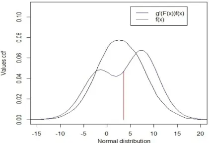
these outcomes can be obtained. It exists several ways of obtaining multi-modal distributions, such as mixing distributions (Gaussian or NIG ones) or distort an initial uni-modal distribution (for instance the Gaussian one) with specific distortion operators. Figure 3 provides an example of such distortion (Wang (2000), Guégan and Hassani (2015)). The objective is to be closer to reality taking into account the information contained in the tails which correspond to the probability of large losses.
Figure 2: This figure presents the density of the Dow Jones Index. We observe that this one cannot be characterised by a Gaussian distribution, or for the matter any distribution that does not capture humps.
Now the objective is to fit a uni-modal distribution on the analysed data sets. We have selected a relatively large panel of classes of distributions to solve this problem. We distinguish two classes of distributions. The first class includes : the lognormal, the Generalised Hyperbolic (GH) (Barndorff-Nielsen (1977)) and the α-stable (Samorodnitsky and Taqqu (1994)). The second class includes the generalised extreme value (Weibull, Fréchet, Gumbel), and the gen-eralised Pareto distributions. It is important to make a distinction between these two classes of distributions as inside the former, the distributions are fitted on the whole sample I while in the latter the distributions are fitted on some specific sub-samples of I: this difference is
Figure 3: This figure presents a distorted Gaussian distribution. We can observe that the weight taken in the body are transferred on the tails.
fundamental in terms of risk management. Note also that the techniques for estimating the parameters of these distributions differ for all these classes of distributions. Besides these two classes of distributions we have also to consider the Empirical distribution fitted on the whole sample using non-parametric techniques. It is the closest fit we can obtain for any data set but bounded by construction, and therefore the extrapolation of extreme exposures in the tails is limited.
Concerning the data set we investigate in this paper, we first fit the Empirical distribution using all the data set, then two other distributions having two parameters - the scale and the shape -, the Weibull and the lognormal distributions. In this exercise we use the whole sample also to fit the Weibull distribution (we analyse latter in this paper the impact of this choice). Then we consider the GH distributions and the α-stable distributions which are nearly equivalent in the sense that they are characterized by five parameters which permit a very good fit on the data set. The difference comes from their definition: we have an explicit form for the density function of the GH, while to work with the α-stable distributions we need to use the moment generating function.
Then we fit extreme value distributions (the generalised extreme value distribution (GEV) and the GPD distribution) which are very appropriate if we want to analyse the probability of ex-treme events without being polluted by the presence of other risks. Indeed, these two types of distributions are defined and built on specific data sets implying the existence of extreme events. The GEV distributions including the Gumbel, Fréchet and Weibull distributions are build as limit distributions characterising a sequence of maxima inside a set of data, thus we need to build this sequence of maxima from the original data set I before estimating the parameters of the appropriate EV distribution. The work has also to be done with the GPD which is built as a limit of distributions existing for data above a certain threshold. Only this subset is used to estimate the parameters of the GPD. Despite this method being widely used, the threshold is always very difficult to estimate and very unstable, thus we would not recommend this distri-bution in practice (or only for a very few cases).
In summary we use the whole sample (original data set) to fit the Weibull, the lognormal, the GH, and the α-stable, as long as maximum likelihood procedures to estimate their parameters, while specific data sets are used as long as a combination of the Hill (Hill (1975)) and maxi-mum likelihood methodologies to estimate the parameters of the GPD distributions; and we use maximum likelihood method associated with a block maxima strategy to parameterise the GEV distributions10. The choice of the distributions cannot be distinguished either from the difficulty of estimating the parameters or the underlying information set. For instance the GPD is very difficult to fit because of the estimation of the threshold which is a key parameter for this family of distributions and is generally very unstable. Besides, the impact of the construction of series of maxima to fit the GEV should not be underestimated. An error in its estimation may bias, distort and confuse both capital calculations and risk management decisions.
It is also important to compare these different parametric adjustments to the empirical distribu-tion (more representative of the past events) and its fitting done using non-parametric techniques (Silverman (1986)). This latter fitting is always useful because if it is done in a very good way, it is generally a good representation of the reality and provides interesting values for the risk
10
measure. It always appears as a benchmark.
These proposals are sometimes quite far from regulatory requirements. Indeed, a very limited class of distributions whose choice seems sometimes arbitrary and not appropriate has been proposed(Guégan and Hassani (2016)). The regulator does not make the distinction between distributions fitted on a whole sample and those which have to be fitted on specific sub-samples. The importance of the information set I is not correctly analysed. Risks of confusion between the construction of the basic model based on the past information set and the possible use of uncertain future events for stress testing exist. Dynamics embedded in risk modelling are not considered and a static approach seems favoured even to analyse long term risk behaviour. Fi-nally, the regulator does not considered the non parametric approach which could be a first basis of discussion with the managers.
We now propose to illustrate our ideas, emphasising the influence of the choice of the distri-butions; how these are fitted and why unstable results can be observed. We show at the same time, the influence of the choice of the level p which is definitively arbitrary. Finally concerning the controversy surrounding the use of the VaR or the ES, we point that, - even if the ES for a given distribution will always provide a larger value for the risk than the VaR - the result in
fine depends on the distribution chosen and the associated level considered.
3
An exercise to convince managers and regulators to consider
a more flexible framework
We have selected a data set provided by a Tier European bank representing an operational risk category risks from 2009 to 2014. This data11 set is characterised by a distribution right skewed (positive skewness) and leptokurtic.
In order to follow regulators’ requirements in their different guidelines, we choose to fit on this data set some of the distributions required by various pieces of regulation as long others
11
In our demonstration, the data set which has been sanitised here is not of particular importance as soon as the same data set has been used for each and every distribution tested.
which seem more appropriate regarding the shape of the data set. As mentioned before, eight distributions have been retained. Fitted on the whole sample (i), the empirical distribution, a lognormal distribution (asymmetric and medium tailed), a Weibull distribution (asymmetric and thin tailed), a Generalised Hyperbolic (GH) distribution (symmetric or asymmetric, fat tailed on an infinite support), an Alpha-Stable distribution (symmetric, fat tailed on an infinite support), a Generalised Extreme Value (GEV) distribution (asymmetric and fat tailed), and the empirical distribution; (ii) on an adequate subset: a Generalised Pareto (GPD) distribution (asymmetric, fat tailed) calibrated on a set built over a threshold, a Generalised Extreme Value (GEVbm) distribution (asymmetric and fat tailed ) fitted using maxima coming from the original set. The whole data set contains 98082 data points, the sub-sample used to fit the GPD contains 2943 data points and the sub-sample used to fit the GEV using the block maxima approach con-tains 3924 data points. The objective of these choices is to evaluate the impact of the selected distributions on the risk representation, i.e. how the initial empirical exposures are captured and transformed by the model. In order to analyse the deformation of the fittings due to the evolution of the underlying data set, the calculation of the risk measures will be performed on the entire data set as long as two sub-samples, splitting the original one. The first sub-sample contains the data from 2009 to 2011 while the second contains the data from 2012 to 2014.
Table 4 exhibits parameters’ estimates for each distribution selected12. The parameters are estimated by maximum likelihood, except for the GPD which implied a Peak-Over-Threshold (Guégan et al. (2011)) approach and the GEV fitted on the maxima of the data set (maxima obtained using a block maxima method (Gnedenko (1943))). The quality of the adjustment is measured using both the Kolmogorov-Smirnov and the Anderson-Darling tests. The results presented in Table 4 shows that none of the distributions are adequate. This is usually the case when we are fitting uni-modal distributions on multi-modal data set. Indeed, the multi-modality of distributions is a frequent issue modelling risks such as operational risks as the unit of mea-sures combine multiple kinds of incidents13. But as illustrated in Figure 3, this phenomenon can also be observed on market or credit data. This is the exact reason why the risk measures are
12
In order not to overload the table the standard deviation of the parameters are not exhibited but are available upon request.
13for instance, a category combining external fraud will contain the fraud card on the body, commercial paper
evaluated, in practice, using the empirical distributions instead of fitted analytical distributions could be of interest as the former one captures multi-modality by construction. Unfortunately this solution has been initially crossed out by regulators as this non-parametric approach is not considered able to capture tails properly, which as shown in the table, might be a false statement. However, recently the American supervisor seems to be re-introducing empirical strategies in practice for CCaR14 purposes. The use of fitted analytical distributions has been preferred despite the fact that sometimes no proper fit can be found and the combination of multiple distributions may lead to a high number of parameters and consequently to even more unstable results. Nevertheless the question of multi-modality becomes more and more important concerning the fitting of any data set. In this paper we do not discuss this issue in any more details as it is out of scope, indeed the regulators never suggested this approach, nevertheless some methodological aspect related to these strategies can be found in Wang (2000) and Guégan and Hassani (2015).
Using the data set and the distributions selected, we compute for each distribution the associ-ated VaRp and ESp for different values of p. The results are provided in Tables 1 - 3.
From Table 1, we see that, given p, the choice of the distribution has a tremendous impact on the value of the risk measure, i.e. if a GH distribution is used, then the 99% VaR is equal to 5 917, while it is 2 439 for a Weibull adjusted on the same data and 84 522 using a GPD. A corollary is that the 90% VaR of the GPD is much higher than all the 99% VaR calculated with any other distribution (considered suitable the case of the GEV will be discussed in the follow-ing). A first conclusion would be, what is the point of imposing a percentile if the practitioners are free to use any distribution (see Operational Risk AMA)? Second, looking at Table 2, for a given p, between the four distributions fitted on the whole sample (lognormal, Weibull, GH and alpha-stable), compared to the GPD fitted above a threshold, we observe a huge difference for the value of the VaR. A change in the threshold may either give higher or lower value, there-fore the VaR is highly sensitive to the value of the threshold. We note also that the Weibull which is a distribution somehow contained in the GEV provides the lowest VaR from the 97.5 percentile. Now, looking at the values obtained regarding the empirical distribution we observe
14
that the values of the risk measures especially in the tail are much larger than those obtained using parametric distributions. These results highlight the fact that the empirical distribution - when the number of data point is sufficiently large - might be suitable to represent a type of exposure, as the embedded information tends to completion.
The values obtained for the ES are also linked to the distribution used to model the underlying risks. Looking at Table 1, at the 95%, we observe that the ES goes from 1 979 for the Weibull to 224 872 for the GPD. Therefore, depending on the distribution used to model the same risk, at the same p level, the ES obtained is completely different. The corollary of that issue is that the ES obtained for a given distribution at a lower percentile will be higher than the ES computed on another distribution at a higher percentile. For example, Table 1 shows that the 90% ES obtained from the empirical distribution is higher than the 97.5% ES computed with a Weibull distribution.
We also illustrated in Table 2 the fact that, depending on the distribution used and the confidence level chosen, the values provided by VaRp can be bigger than the values derived for an ESp and conversely. Thus a question arises: What should we use the VaR or the Expected Shortfall? To answer to this question we can consider several points:
• Conservativeness: Regarding that point, the choice of the risk measure is only relevant for a given distribution, i.e. for any given distribution the VaRp will always be inferior to the ESp (assuming only positive values) for a given p. But, if the distribution used to characterise the risk has been chosen and fitted, then it may happen that for a given level
p, the VaRp obtained from a distribution is superior to the ESp.
• Distribution and p impacts: Table 1 shows that potentially a 90% level ES obtained on a given distribution is larger than a 99.9% VaR obtained on another distribution, e.g. the ES obtained from a GH distribution at 90% is higher that the VaR obtained form a lognormal distribution at 97.5%. Thus is it always pertinent to use a high value for p?
• Parameterisation and estimation: the impact of the calibration of the estimates of the parameters is not negligible (Neslehova et al. (2006) and Guégan et al. (2011)), mainly when we fit a GPD. Indeed in that latter case, due to the instability of the estimates for
the threshold, the practitioners can largely overfit the risks. Thus, why the regulators still impose this distribution?
• It seems that regulators impose these rules to avoid small banks lacking personnel to build an internal model abusing the system. This attitude is quite dangerous as it removes the accountability from them, they should definitely incentivise to do the measurement themselves, it lacks realism considering that managers are more and more prepare to build appropriate models and the industry needs to use them and to innovate. We would recom-mend regulator to follow the same path. By innovating banks will see their risk framework maturing and their natural accountability will push them to a better understanding of the risk they are taking.
Now regarding the impact of the choice of the information sets on the calculation of the con-sidered risk measure, need to be commented. First, results obtained from the GPD and the
α-stable distribution are of the same order whatever the information set. Second, the differences
between the GPD and the GEV fitted on the block maxima are huge, illustrating the fact that despite being two extreme value distributions, the information captured is quite different. We analyse now in more detais the results based on the different data sets.
Table 1 shows that the 90% VaRs are of the same order for all the distributions presented except the GPD and the GEV. For the former, the fact that we use a sub-sample of the initial data set superior to a threshold u, the 0% VaR of the GPD is already equal to u and that makes it difficult to compare with other distributions as the support is shifted from (0; +∞) to [u; +∞). For the GEV, we have a parameterisation issue as the shape parameter ξ ≤ 1 characterises an infinite mean model (Table 4), therefore we will not comment any further the results presented in the first table with respect to this distribution. Though the empirical distribution seems always showing lower VaR values, this is not always true for high percentiles. Indeed, the larger the data points in the tails, the more explosive will be the upper quantiles. Here, the 99.9% VaR is larger than the one provided by the lognormal, the Weibull, or the GH. Therefore, if conservatisme is our objective and we want to use the entire data set only the α-stable distribution is suitable. In the meantime, the construction of an appropriate series of maxima to apply a GEV seems promising as it captures the tail while still being representative of smaller percentiles. Regarding
the Expected Shortfall, we see once again that the lognormal and the Weibull do not allow to capture the tails as the values are all lower than the empirical expected shortfall. The GH is not too far from the empirical ES though, the tail of the fitted GH is not as thick as the empirical. The GPD is once again out of range, though, a combination of the empirical distribution and a GPD may lead to appropriate results as the percentile would mechanically decrease (Guégan et al. (2011)).
Regarding Table 2 the comments are fairly similar to those for Table 1. From a VaR point of view, the most appropriate distribution are the GEV and the α-stable. This is somehow quite unexpected as the GEV fitted on the entire data-set was only used here as a benchmark to the GEV fitted on the series of Maxima. Though, these two distributions are not considered reliable regarding the ES as both have infinite first moment, (as α < 1 for the α-stable and ξ > 1 for the GEV (Table 5)).
Looking at Table 3 we can note that the best fit from a VaR point of view is the GH, though this is not true anymore from an ES perspective. In the particular case none of the distributions seems appropriate as three of them have infinite means except maybe the GPD, but this one taken on a support [u, +∞) provides results not comparable with empirical distribution (Table 6).
Dynamically speaking, we observe now that the fittings on various periods of time does not pro-vide the same results for any of the distribution. If some are of the same order and fairly stable especially for the largest quantiles, these may differ largely. Some distributions such as the GEV are not always appropriate over time though the underlying data are supposed to provide dra-matically different features from a period to another one. The extreme tail is far larger for the empirical distribution for the period 2012-2014 than for the previous one or the whole sample. Besides except for the GH, the fitted distribution are providing even lower risk measures for the third sub-sample than for any of the other ones which implies that the right15 tail is definitely not captured. It also tells us that no matter how good is a fit of a distribution, this one is always obtained at a time t and is absolutely not representative of the "unknown" entire information set.
15
Another interesting point is the fact that though the VaR is criticised, this one allows the use of more distribution than the ES which requires to have a finite first moment. Indeed, the ES theoretically captures the information contained in the tail in a better fashion, in our case most of the fat-tailed distribution have an infinite mean which leads to unreliable ES even if calculated on a randomly generated sample.
In summary, we think that a risk measure which is not correctly computed and interpreted can lead to catastrophes, ruins, failures, etc. because of an inappropriate management, control and understanding of the risks associated in banks. In this paper, we have focused on the fact that it is important to have an holistic approach in terms of risks including the knowledge of the appro-priate distribution, the choices of different risk measures, a spectral approach in terms of levels and a dynamic analysis. Nevertheless, various problems remain open, in particular those related to estimation procedures, such as (i) the empirical bias of skewness and kurtosis calculation, (ii) the dependence between the distributions’ parameters, (iii) their impact on the estimation of the quantile computed from the fitted distributions and (iv) the construction of a multivariate VaR and ES. In another side, in this paper multivariate approaches are not discussed, i.e. the computation of risk measures in higher dimensions as this will be the contents of a companion paper. Besides, the question of diversification linked to the notion of sub-additivity is not also the core of this paper and will be discussed in another paper as long as the problem of aggre-gation of risks for which we just provide here an illustration pointing the impact of false ideas implied by Basel guidelines on the computation of capital requirements.
In conclusion, the issues highlighted in this paper are quite dramatic as enforcing the wrong risk measurement strategy (to be distinguished from the wrong risk measures) may lead to dramatic issues. First, if the strategy is used for capital calculations then, we would have a mismatch between the risk profile and the capital charge supposed to cover it. Second, if the strategy is used for risk management, the controls implemented will be inappropriate and therefore the institution at risk. Finally, the cultural impact of enforcing some risk measurement approaches leads to the creation of so-called best practices, i.e. the fact that all the financial institutions
are applying the same methods, and if these are inappropriate, then the combination of having all the financial institutions at risk simultaneously will lead to a systemic risk.
References
Barndorff-Nielsen, O. (1977), ‘Exponentially decreasing distributions for the logarithm of par-ticle size’, Proceedings of the Royal Society of London. Series A, Mathematical and Physical
Sciences (The Royal Society) 353 (1674), 401–409.
BCBS (1995), ‘An internal model-based approach to market risk capital requirements’, Basel
Committee for Banking Supervision, Basel .
BCBS (2011), ‘Interpretative issues with respect to the revisions to the market risk framework’,
Basel Committee for Banking Supervision, Basel .
EBA (2014), ‘Draft regulatory technical standards on assessment methodologies for the advanced measurement approaches for operational risk under article 312 of regulation (eu) no 575/2013’,
European Banking Authority, London .
Gnedenko, B. (1943), ‘Sur la distribution limite du terme d’une série aléatoire’, Ann. Math.
44, 423–453.
Guégan, D. . and Hassani, B. (2016), ‘Risk measures at risk- are we missing the point? -discussions around sub-additivity and distortion’, Working paper, Université Paris 1 .
Guégan, D. and Hassani, B. (2015), Distortion risk measures or the transformation of unimodal distributions into multimodal functions, in A. Bensoussan, D. Guégan and C. Tapiro, eds, ‘Future Perspectives in Risk Models and Finance’, Springer Verlag, New York, USA.
Guégan, D., Hassani, B. and Naud, C. (2011), ‘An efficient threshold choice for the computation of operational risk capital.’, The Journal of Operational Risk 6(4), 3–19.
Hill, B. M. (1975), ‘A simple general approach to inference about the tail of a distribution’, Ann.
Statist. 3, 1163 – 1174.
Neslehova, J., Embrechts, P. and Chavez-Demoulin, V. (2006), ‘Infinite mean models and the lda for operational risk’, Journal of Operational Risk 1.
Riskmetrics (1993), ‘Var’, JP Morgan .
Samorodnitsky, G. and Taqqu, M. (1994), Stable Non-Gaussian Random Processes: Stochastic
Models with Infinite Variance, Chapman and Hall, New York.
Silverman, B. W. (1986), Density Estimation for statistics and data analysis, Chapman and Hall/CRC, London.
Wang, S. S. (2000), ‘A class of distortion operators for pricing financial and insurance risks.’,
%tile Distribution Empirical LogNormal W eibull GPD GH Alpha-Stable GEV GEVbm V aR ES V aR ES V aR ES V aR ES V aR ES V aR ES V aR ES V aR ES 90% 575 2 920 686 2 090 753 1 455 10 745 146 808 627 2 950 582 29 847 + ∞ 2.097291e+06 + ∞ 626 12 755 95% 1 068 5 051 1 251 3 264 1 176 1 979 19 906 224 872 1 317 5 006 1 209 58 872 + ∞ 2.869971e+07 + ∞ 1 328 24 616 97 .5% 1 817 8 775 2 106 4 925 1 674 2 572 37 048 368 703 2 608 8 187 2 563 116 016 + ∞ 3.735524e+08 + ∞ 2 762 47 356 99% 3 662 18 250 3 860 8 148 2 439 3 468 84 522 758 667 5 917 14 721 7 105 283 855 + ∞ 1.073230e+10 + ∞ 7 177 111 937 99 .9% 31 560 104 423 13 646 24 784 4 852 6 191 675 923 5 328 594 28 064 46 342 98 341 2 649 344 + ∞ 4.702884e+13 + ∞ 77 463 945 720 T able 1: Univ ariate Risk Measures -This table exhibits the V aRs and ESs for the heigh t typ es of distributions considered -empirical, lognormal, W eibull, GPD, GH, α -stable, GEV and GEV fitted on a series of maxima -for fiv e c on fidence lev el (90%, 95%, 97.5%, 99% an d 99.9%) e v aluated on the p erio d 2009-2014. Note that the parameters obtained for the α -stable and the GEV fitted on the en tire data set lead to infinite mean mo del and therefore, the ES are hardly applicable.
%tile Distribution Empirical LogNormal W eibull GPD GH Alpha-Stable GEV GEVbm V aR ES V aR ES V aR ES V aR ES V aR ES V aR ES V aR ES V aR ES 90% 640 2 884 738 2 238 803 1 542 11 378 137 154 686 2 925 625 15 237 + ∞ 676 10 130 + ∞ 2 557 74 000 989 + ∞ 95% 1 086 4 965 1 344 3 492 1 249 2 093 20 994 204 873 1 432 4 874 1 283 29 652 + ∞ 1 438 19 292 + ∞ 7 414 147 997 711 + ∞ 97 .5% 1 953 8 387 2 259 5 265 1 771 2 714 38 938 327 418 2 788 7 784 2 684 57 580 + ∞ 2 999 36 538 + ∞ 21 053 295 983 188 + ∞ 99% 4 006 16 993 4 133 8 693 2 570 3 639 88 471 652 229 6 014 13 442 7 311 137 784 + ∞ 7 821 84 287 + ∞ 82 476 739 897 783 + ∞ 99 .9% 30 736 86 334 14 561 26 378 5 078 6 384 700 863 4 182 440 24 409 37 774 96 910 1 184 005 + ∞ 85 225 658 076 + ∞ 2 494 850 7 395 636 153 + ∞ T able 2: Univ ariate Risk Measures -This table exhibits the V aRs and ESs for the heigh t typ es of distributions considered -empirical, lognormal, W eibull, GPD, GH, α -stable, GEV and GEV fitted on a series of maxima -for fiv e c on fidence lev el (90%, 95%, 97.5%, 99% and 99.9%) ev alu ate d on the p erio d 2009-2012. Note that the parameters obtained for the α -stable, the GEV fitted on the en tire data set and the GEV fitted on the series of maxima (GEVbm) lead to infinite mean mo del and th e refore, the ES ar e hardly applicable.
%tile Distribution Empirical LogNormal W eibull GPD GH Alpha-Stable GEV GEVbm V aR ES V aR ES V aR ES V aR ES V aR ES V aR ES V aR ES V aR ES 90% 501 3 002 568 1 722 637 1 246 9 269 121 928 494 3 006 504 336 621 + ∞ 504 6 578 2 063 3 009 981 + ∞ 95% 906 5 344 1 034 2 688 1 002 1 702 17 197 176 742 1 035 5 308 1 060 672 418 + ∞ 1 044 12 442 6 021 6 016 460 + ∞ 97 .5% 1 397 9 625 1 739 4 057 1 435 2 222 31 868 275 836 2 129 9 162 2 272 1 343 100 + ∞ 2 122 23 416 17 206 12 022 771 + ∞ 99% 2 967 21 048 3 182 6 702 2 103 3 003 71 958 537 693 5 186 18 043 6 380 3 351 534 + ∞ 5 345 53 611 67 972 30 005 581 + ∞ 99 .9% 32 977 145 966 11 211 19 917 4 232 5 387 556 192 3 405 540 36 582 74 465 90 939 33 319 684 + ∞ 53 329 411 769 2 099 862 297 164 627 + ∞ T able 3: Univ ariate Risk Measu res -This table exhibits the V aRs and ESs the heigh t typ es of distributions considered -empirical, lognormal, W eibull, GPD, GH, α -stable, GEV and GEV fitted on a series of maxima -for fiv e c on fidence lev el (90%, 95%, 97.5%, 99% an d 99.9%) e v aluated on the p erio d 2012-2014. Note that the parameters obtained for the α -stable and the GEV fitted on the series of maxima (GEVbm) lead to infinite mean mo d e l and therefore, the ES are hardly applicable.
P arameters Distribution lognormal W eibull GPD GH α -Stable GEV GEVbm µ 4.412992 -1541.558 -5.5846599 -587.855749 50.272385 σ 1.653022 -2137.940297 64.720971 α -0.5895611 -0.1906536 0.86700 -β -182.9008432 1185.8083087 0.1906304 0.95000 -ξ -0.9039617 -3.634536 1.030459 δ -22.5118547 58.18019 -λ --0.871847 -γ -54.21489 -KS < 2.2e-16 < 2.2e-16 < 2.2e-16 < 2.2e-16 < 2.2e-16 < 2.2e-16 < 2.2e-16 AD 6.117e-09 6.117e-09 6.117e-09 NA 6.117e-09 (d) 6.117e-09 6.117e-09 T able 4: This table pro vides the estimated parame ters for the sev en parametric distributions fitted on the whole sample 2009 -2014. If for the α stable distribution α < 1 , for the GEV, GEVbm and for GPD ξ > 1 , w e are in the presence of an infinite mean mo del. The p-v alues of b oth K olmogoro v-Smirno v and Anderson-Darling tests are also pro vided for the fit of eac h distribution.
P arameters Distribution lognormal W eibull GPD GH α -Stable GEV GEVbm µ 4.491437 -1673.466 -6.7360463 -54.015458 89.133874 σ 1.648636 -69.462437 136.011312 α -0.5955548 -0.2356836 0.88100 -β -197.8528740 1257.9298250 0.2356488 0.95000 -ξ -0.9000192 -1.034631 1.477802 δ -20.7002703 61.74123 -λ --0.8431451 -γ -60.64299 -KS < 2.2e-16 < 2.2e-16 < 2.2e-16 < 2.2e-16 < 2.2e-16 < 2.2e-16 < 2.2e-16 AD 6.117e-09 6.117e-09 6.117e-09 NA 6.117e-09 (d) 6.117e-09 6.117e-09 T able 5: This table pro vides the estimated parame ters for the sev en parametric distributions fitted on the whole sample 2009 -2011. If for the α stable distribution α < 1 , for the GEV, GEVbm and for GPD ξ > 1 , w e are in the presence of an infinite mean mo del. The p-v alues of b oth K olmogoro v-Smirno v and Anderson-Darling tests are also pro vided for the fit of eac h distribution.
P arameters Distribution lognormal W eibull GPD GH α -Stable GEV GEVbm µ 4.229681 -1153.398 -3.6045095 -42.8811564 70.934898 σ 1.648738 -54.5957915 108.146149 α -0.5800014 -0.1418024 0.85800 -β -151.1403422 1071.578078 0.1417962 0.95000 -ξ -0.887863 -0.9961461 1.486931 δ -25.0230238 45.83589 -λ --0.9400653 -γ -46.11706 -KS < 2.2e-16 < 2.2e-16 < 2.2e-16 < 2.2e-16 < 2.2e-16 < 2.2e-16 < 2.2e-16 AD 6.117e-09 6.117e-09 6.117e-09 NA 6.117e-09 (d) 6.117e-09 6.117e-09 T able 6: This table pro vides the estimated parame ters for the sev en parametric distributions fitted on the whole sample 2012 -2014. If for the α stable distribution α < 1 , for the GEV, GEVbm and for GPD ξ > 1 , w e are in the presence of an infinite mean mo del. The p-v alues of b oth K olmogoro v-Smirno v and Anderson-Darling tests are also pro vided for the fit of eac h distribution.