HAL Id: halshs-00587779
https://halshs.archives-ouvertes.fr/halshs-00587779
Submitted on 21 Apr 2011
HAL is a multi-disciplinary open access archive for the deposit and dissemination of sci-entific research documents, whether they are pub-lished or not. The documents may come from teaching and research institutions in France or abroad, or from public or private research centers.
L’archive ouverte pluridisciplinaire HAL, est destinée au dépôt et à la diffusion de documents scientifiques de niveau recherche, publiés ou non, émanant des établissements d’enseignement et de recherche français ou étrangers, des laboratoires publics ou privés.
The Riskiness of Risk Models
Christophe Boucher, Bertrand Maillet
To cite this version:
Documents de Travail du
Centre d’Economie de la Sorbonne
The Riskiness of Risk Models
Christophe BOUCHER, Bertrand MAILLET
“The Riskiness of Risk Models”
*Christophe M. Boucher♦ Bertrand B. Maillet♦♦
- March 2011 -
We provide an economic valuation of the riskiness of risk models by directly measuring the impact of model risks (specification and estimation risks) on VaR estimates. We find that integrating the model risk into the VaR computations implies a substantial minimum correction of the order of 10-40% of VaR levels. We also present results of a practical method – based on a backtesting framework – for incorporating the model risk into the VaR estimates.
Keywords: Model Risk; Quantile Estimation; VaR; Basel II Validation Test. JEL Classification: C14, C50, G11, G32.
* We here acknowledge Monica Billio, Massimiliano Caporin, Rama Cont, Christophe Hurlin, Christophe Pérignon, Michaël Rockinger, Thierry Roncalli and Jean-Michel Zakoïan for suggestions when preparing this work, as well as Vidal Fuentes, Benjamin Hamidi and Patrick Kouontchou for helpful discussions, research assistance and joint collaborations on collateral subjects. The first author thanks the Banque de France Foundation and the second the Europlace Institute of Finance for financial support. The usual disclaimer applies.
♦ A.A.Advisors-QCG (ABN AMRO), Variances and University of Paris-1 (CES/CNRS); E-mail:
♦♦ A.A.Advisors-QCG (ABN AMRO), Variances and University of Paris-1 (CES/CNRS and EIF).
Correspondance to: Bertrand Maillet, CES/CNRS, MSE, 106-112 Bd de l’Hôpital F-75647 Paris Cedex 13. Tel.: +33 144078189/70 (fax). Mail: [email protected].
1. Introduction
The recent worldwide financial crisis has dramatically revealed that risk
management pursued by financial institutions is far from optimal. This paper
proposes an economic evaluation of the impact of model uncertainty on VaR
estimates based on a backtesting framework.
The Basel III committee has recently further proposed that financial institutions
assess the model risk (BCBS, 2009). However, the model risk, whilst well studied
in the case of specific price processes (e.g. Cont, 2006), is not yet taken into
account practically in the building of risk models by the industry1.
The outline of the paper is as follows. Section 2 defines and illustrates the
model risk in VaR estimates. Section 3 presents our practical approach for
calibrating adjusted Empirical VaRs that deal with the model risk. Section 4
concludes.
2. Model Risk and VaR Computations
We first illustrate the model risk of VaR estimates, which is here defined
as the consequence of two types of errors due to a model misspecification and a
1 Only a few recent papers (e.g. Kerkhof et al., 2010; Gouriéroux and Zakoïan, 2010) still aim to take
parameter estimation uncertainty. Various VaR computation methods do indeed
exist in the literature, from non-parametric, semi-parametric and parametric
approaches (e.g. Christoffersen, 2009). However, the Historical-simulated VaR
computation is still the one most used by practitioners (Christoffersen and
Gonçalves, 2005) and will serve as the reference throughout this article.
Table 1 presents the Estimated VaR as well as the mean, minimum and
maximum errors on these Estimated VaR. Errors are defined by the differences
between the “true” asymptotic VaR (based on simulated DGP) and the Imperfect
Historical-simulated Estimated VaR (because the latter are approximately
specified and estimated with a limited data sample). Three different rolling
time-windows (from 250 to 750 days in Panels A, B and C) and several levels of
probability confidence thresholds (three rows for each Panel) are considered. The
results are presented for three Data Generating Processes for the underlying stock
price with various intensities of jumps (Brownian, Lévy and Hawkes2
).
As expected, the Estimated VaR is an increasing function of the
confidence level and the presence of jumps in the process (Lévy and Hawkes’
cases). For a large number of trials, the mean bias of the Historical-simulated
Method is quite small (inferior to 1% in relative terms) in the Brownian case, and
rather insensitive to the number of datapoints in the sample. By contrast, this
mean bias is quite large when jumps are considered (with an amplitude of 10% to
27% in relative terms3
).
Moreover, the observed range of potential relative errors (the difference
between the maximum and minimum estimated errors divided by the estimated
VaR) is substantial in our experiments, representing between around 40% of the
VaR levels in the best case (for the simple Brownian DGP over the longer
sample) to as high as 290% in the worst case scenario (for the Lévy DGP over the
shorter sample). Furthermore, the potential relative under-estimation of the
“true” VaR (too aggressive estimated VaR) is, in the main, large (ranging from
13% to 40%, depending on the sample length and the quantile considered4
). These
results suggest that the Historical-simulated VaR should be corrected when safely
taking into account the riskiness of risk models.
3 The relative error of 27% corresponds to the probability 99.50% with a window of 250 days for the
Lévy DGP (i.e. 14.90 out of -54.26).
4 The relative error of 40% corresponds to the probability 99.50% with a window of 250 days for the
Table 1
Estimated annualized VaR and model-risk errors (%)
Three price processes of the asset returns are considered below, such as for t=[1,…,T] and p=[1, 2, 3]:
(
t pt t)
t t S dt dW J dN dS = µ +σ + with: ( ) ( ) [ ] − − + = − = = ) . 3 ( exp ) . 2 ( exp ) . 1 ( 0 3 3 2 2 2 1 Hawkes s t J Lévy t J Brownian J t t t γ β λ λ λwhere St is the price of the asset at time t, Wt is a standard Brownian motion, independent from the Poisson process Nt,
governing the jumps of various intensities Jpt (null, constant or time-varying according to the process p), defined by
parameters, λ2, λ3, β and γ, which are some positive constants, with s (in case 3) the date of the last observed jump.
Processes 1. Brownian 2. Lévy 3. Hawkes
VaR and Error (in %): Mean Estimate d VaR Mean VaR Error Min VaR Error Max VaR Error Mean Estimated VaR Mean VaR Error Min VaR Error Max VaR Error Mean Estimated VaR Mean VaR Error Min VaR Error Max VaR Error Probabilit
y Panel A. One-year Rolling Window Calibration (T=250)
95.00% -24.78 -0.06 -8.69 10.16 -25.18 2.49 -6.53 15.28 -27.33 3.51 -6.52 25.25 99.00% -35.74 -0.11 -14.21 20.70 -39.07 5.07 -12.35 101.73 -44.78 7.47 -14.64 61.16 99.50% -39.95 0.09 -16.04 28.92 -54.26 14.90 -14.60 122.56 -54.16 9.14 -19.50 65.39
Panel B. Two-year Rolling Window Calibration (T=500)
95.00% -24.81 -0.03 -6.25 7.34 -25.20 2.51 -3.63 10.29 -26.87 3.05 -4.77 15.03 99.00% -35.85 0.00 -10.04 14.45 -38.18 4.19 -7.73 75.61 -43.35 6.04 -11.03 43.80 99.50% -39.81 -0.06 -12.66 19.97 -49.60 10.24 -12.15 102.05 -52.28 7.26 -16.88 54.31
Panel C. Three-year Rolling Window Calibration (T=750)
95.00% -24.82 -0.03 -5.56 5.99 -25.21 2.52 -3.26 8.63 -26.72 2.89 -3.43 12.40 99.00% -35.86 0.01 -8.54 11.29 -37.86 3.87 -6.05 66.22 -42.69 5.37 -8.34 39.40 99.50% -39.90 0.03 -10.61 14.57 -48.38 9.02 -8.94 93.76 -51.85 6.84 -13.83 45.78 Source: simulations by the authors. Errors are defined as the difference between the “true” asymptotic simulated VaR and the Estimated VaR. These statistics were computed with a series of 250,000 simulated daily returns with specific DGP (1. Brownian, 2. Lévy and 3. Hawkes), averaging the parameters estimated in Aït-Sahalia et al. (2010, Table 5, i.e. β=41.66%,
λ3=1.20% and γ=22.22%), and ex post recalibrated for sharing the same first two moments (i.e. µ=.12% and σ=1.02%) and
the same mean jump intensity (for the two last processes such as 2 3
t t J
J = - which leads after rescaling here, for instance, to an
intensity of the Levy such as: λ2=1.06%). Per convention, a negative adjustment term in the table indicates that the
Estimated VaR (negative return) should be more conservative (more negative).
3. A Simple Procedure for adjusting Estimated VaR
We propose herein a simple procedure to calibrate a correction on VaR
estimates to account for the impact of the model errors. This procedure is based
backtesting process is carried out by comparing the last 250 daily 99% VaR
estimates with corresponding daily trading outcomes.
The regulatory framework uses the proportion of a failure test based on the
Unconditional Coverage test (Kupiec, 1995). This test is based on the so-called
“hit variable” associated to the ex post observation of Estimated VaR violations
at the threshold α and time t, denoted ItEVaR(α), which is defined such:
( ). ( ) 1 if
(
,)
1 0 otherwise, EVaR t t t r EVaR P I α α − < − = (1)where EVaR
()
. is the Estimated VaR on a portfolio P at a threshold α , and rt is thereturn on a portfolio P at time t, with t=
[
1,...,T]
.If we assume that the ItEVaR(⋅) variables are Independently and Identically
Distributed, then, under the unconditional coverage hypothesis (Kupiec, 1995), the
total number of VaR exceptions (Cumulated Hits) follows a Binomial distribution
(Christoffersen, 1998), denoted B(T,α), such as:
()
∑
() ( )
(
)
= →>+∞ = T t T B T EVaR t I EVaR T Hit 1 , ~ . . α α (2)A Perfect VaR (not too aggressive, but not too confident) in the sense of
this test, is such that it provides a sequence of VaR denoted VaR
()
.* (i.e. all(
)
{
*}
, t
( ) ( ) ≥ + < − − , 1 * * . 1 . 1 α α VaR T VaR T Hit T Hit T (3)
where HitVaRT (.)*(⋅) is the cumulated hit variable associated to the VaR
( )
. *.In other words, since the Estimated VaR and the bounding range are known, we now have to search, amongst all possibilities, for the minimum (unconditional) adjustment that allows us to recover a Corrected Estimated VaR that respects condition (3) over the whole sample, i.e.:
(
)
{
(
)
}
( ) ( )(
)
(
)
* * * * * . 1 . 1 * * , , . .: 1 , : , , . t q IR VaR T VaR T t tadj P q ArgMax VaR P
s t T Hit T Hit with VaR P EVaR P q α α α α α α ∈ − − = = < + ≥ = + (4)
Figure 1 represents the minimum adjustments (absolute errors) to be
applied to estimated VaR, denoted q* as solutions of the optimization program (4),
for one-year (two-year and three-year) Historical-simulated VaR computed on the
DJIA over more than one century (from the 1st
of January, 1900 to the 15th
of
October, 2010). In other words, it represents the minimal global constants that we
should have added to the quantile estimations for having reached a VaR sequence
confidence. We observe that the Historical-simulated error is quite significant for all
quantiles (between -0.5% and -7% in absolute terms, i.e. 15% or so in relative terms)
and significantly increases with the confidence level.
Figure 1
Minimum Model Risk Adjustments associated to Historical-simulated VaR
Source: Bloomberg; daily data of the DJIA index in USD from the 1st January 1900 to the 15th October 2010; computations by the authors. The first plot (on the left hand side) represents the non-adjusted average annualized VaR level. The minimal adjustment is represented in the second plot and is expressed in absolute value (on the right hand side). The minimal adjustment necessary to respect the hit ratio criterion is here considered as a proxy of the economic value of the model risk. The historical VaR is computed on a daily horizon as an annualized empirical quantile using respectively 1 year, 2 years and 3 years of past returns. Without any adjustment, the imperfect Estimated VaR is underestimated (too permissive) in each of these cases.
Besides, the smaller the estimation period, the more important the
adjustment (both in absolute and relative terms). This phenomenon can be explained
by the fact that using larger estimation periods leads more likely to take into
consideration extreme realizations and crisis episodes.
4. Conclusion
This paper proposes a practical method to incorporate model risk into risk
measure estimates by adjusting the estimated VaR according to the frequency of
past exceptions. This VaR adjustment allows a joint treatment of theoretical and
estimation risks, taking into account their possible dependence.
We find that the model risk can represent a significant part of the risk
measure in simulations and, secondly, that the required correction may be
substantial (of the order of 10-40% of VaR levels in extensive simulations, and in
the range of 1-15% for a real risky stock market index). Recently, this kind of bias
estimation and correction of risk measures has been proposed by Kerkhof et al.
(2010) with a similar range of estimated corrections based on different DGP.
References
Aït-Sahalia, Y., Cacho-Diaz, Laeven, R.J., 2010. Modeling Financial Contagion using Mutually Exciting Jump Processes. Princeton Working Paper, 69 pages.
Applebaum, D., 2004. Lévy Processes - From Probability to Finance and Quantum Groups, Notices of the American Mathematical Society 51(11), 1336-1347.
Basel Committee on Banking Supervision, 1996. Amendment to the Capital Accord to Incorporate Market Risks. Bank for International Settlements, 63 pages.
Basel Committee on Banking Supervision, 2009. Revisions to the Basel II Market Risk Framework, Bank for International Settlements, 35 pages.
Christoffersen P., 2009. Value-at-Risk Models, in: Andersen, T.G., Davis, R.A., Kreiss, J-P., Mikosch, T. (Eds.), Handbook of Financial Time Series, Springer Verlag, 753-766.
Christoffersen P., 1998. Evaluating Interval Forecasts, Int. Econ. Rev. 39(4), 841-862. Christoffersen, P., Gonçalves, S. 2005, Estimation Risk in Financial Risk
Management, Journal of Risk 7(3), 1-28.
Cont, R. 2006. Model Uncertainty and its Impact on the Pricing of Derivative Instruments, Math. Finance 16(3), 519-547.
Gouriéroux, C., Zakoïan, J-M., 2010. Estimation Adjusted VaR”, mimeo CREST, 39 pages.
Kerkhof, J., Melenberg, B., Schumacher, H., 2010. Model Risk and Capital Reserves, J. Banking Finance 34(1), 267-279.
Kupiec, P.H., 1995. Techniques for Verifying the Accuracy of Risk Measurement Models, J. Derivatives 3(2), 73-84.
Appendix. Complementary Results at the Referees’ Attention.
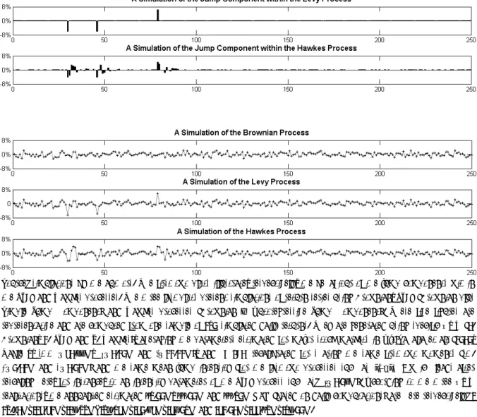
Figure A1 presents simple illustrations on a limited series of 250 returns of the behaviours of the three underlying processes (Brownian, Levy and Hawkes) used in Table 1.
Figure A1
An Illustration of Simulated Processes used in Table 1 for a Series of 250 Returns
Source: simulations by the authors. The first two plots illustrate, respectively, the behaviour of the jump components within the Lévy and Hawkes processes. The three last plots present simulations of return series using Brownian, Lévy (Brownian plus Simple Jump Component) and Hawkes processes (Brownian + Autoregressive Jump Component). These five figures are representative and are computed from one sample of 250 simulated daily returns. They are generated using specific DGP (1. Brownian, 2. Lévy and 3. Hawkes), averaging the parameters estimated for major stock markets in Aït-Sahalia et al. (2010, Table 5, i.e. β=41.66%, λ3=1.20% and γ=22.22%), and ex post recalibrated for sharing the same first two moments (i.e.
µ=0.12% and σ=1.02%) and the same mean jump intensity (for the last two processes such as 2 3
t
t J
J = - which leads after rescaling here, for instance, to an intensity parameter of the Lévy process such as: λ2=1.06%). According to the three DGP
realizations, the annualized estimated 95.00%, 99.00% and 99.50% VaR (based on daily computations) are here respectively: -23.81%/-24.42%/-26.33%; -38.54%/-40.74%/-47.05% and -42.01%/-44.93%/-56.00%.
The Table A1 confirms the convergence of the results presented in the
corpus of the text (see Table 1). We independently reproduced Table 1 with
another set of 250,000 simulations and show the resulting differences for each cell. Except in three cases, most of the relative differences are below 1.00%, and none are above 5.00%.
Table A1
Differences between Results in Two Sets of 250,000 Times-series of Computations reported in Table 1
Three price processes of the asset returns5 are considered below, such as for t=[1,…,T] and p=[1, 2, 3]:
+ + = JptdNt t dW dt t S t dS µ σ with: ( ) ( ) [ ] − − + = − = = ) . 3 ( exp ) . 2 ( exp ) . 1 ( 0 3 3 2 2 2 1 Hawkes s t J Lévy t J Brownian J t t t γ β λ λ λ
where St is the price of the asset at time t, Wt is a standard Brownian motion, independent from the Poisson process Nt,
governing the jumps of various intensities Jpt (null, constant or time-varying according to the process p), defined by parameters,
λ2, λ3, β and γ, which are some positive constants, with s (in case 3) the date of the last observed jump.
Processes: 1. Brownian 2. Lévy 3. Hawkes
VaR and Error (in %): Mean Estimated VaR Mean VaR Error Min VaR Error Max VaR Error Mean Estimated VaR Mean VaR Error Min VaR Error Max VaR Error Mean Estimated VaR Mean VaR Error Min VaR Error Max VaR Error Probability Panel A. One-year Rolling Window Calibration (T=250)
95.00% -0.26 0.00 -0.10 0.09 -0.26 0.01 -0.08 0.14 -0.28 0.02 -0.08 0.24
99.00% -0.37 -0.02 -0.15 0.20 -0.40 0.04 -0.13 1.01 -0.46 0.06 -0.16 0.60
99.50% -0.41 0.01 -0.17 0.28 -0.55 0.14 -0.16 1.21 -0.55 0.08 -0.21 0.64
Panel B. Two-year Rolling Window Calibration (T=500)
95.00% -0.26 0.00 -0.07 0.06 -0.26 0.01 -0.05 0.09 -0.28 0.02 -0.06 0.14
99.00% -0.37 -0.18 -0.11 0.13 -0.39 0.03 -0.09 0.75 -0.44 0.05 -0.12 0.43
99.50% -0.41 -0.04 -0.14 0.19 -0.51 0.09 -0.13 1.01 -0.53 0.06 -0.18 0.53
Panel C. Three-year Rolling Window Calibration (T=750)
95.00% -0.26 0.01 -0.07 0.05 -0.26 0.01 -0.04 0.08 -0.28 0.02 -0.04 0.11
99.00% -0.37 0.03 -0.10 0.10 -0.39 0.03 -0.07 0.65 -0.44 0.04 -0.09 0.38
99.50% -0.41 0.04 -0.12 0.14 -0.49 0.08 -0.10 0.93 -0.53 0.06 -0.15 0.45
Source: simulations by the authors. This table presents the differences (in relative terms expressed in %) between results in two Sets of 250,000 Times-series as a robustness check of the convergence of computations of Imperfect Historical-simulated Estimated VaR and Model-risk Errors as reported in Table 1, using the very same methodology explained in the source of Table 1 in the corpus of the text. Except in three cases, most of the relative differences are below 1.00%. and none are above 5.00%.
The following Table A2 (similar to Table 1, but with a weekly frequency of observations) checks the influence of the jump autocorrelation structure in the Hawkes Process onto the VaR Levels. Since shocks may accumulate during a week, the VaR get worse when a Hawkes process is considered.
Table A2
Estimated VaR and Model-risk Errors based on Weekly Returns (%)
Three price processes of the asset returns are considered below, such as for t=[1,…,T] and p=[1, 2, 3]:
(
t pt t)
t t S dt dW J dN dS = µ +σ + with: ( ) ( ) [ ] − − + = − = = ) . 3 ( exp ) . 2 ( exp ) . 1 ( 0 3 3 2 2 2 1 Hawkes s t J Lévy t J Brownian J t t t γ β λ λ λwhere St is the price of the asset at time t, Wt is a standard Brownian motion, independent from the Poisson process Nt,
governing the jumps of various intensities Jpt (null, constant or time-varying according to the process p), defined by
parameters, λ2, λ3, β and γ, which are some positive constants, with s (in case 3) the date of the last observed jump.
Processes 1. Brownian 2. Lévy 3. Hawkes
VaR and Error (in %): Mean Estimated VaR Mean VaR Error Min VaR Error Max VaR Error Mean Estimated VaR Mean VaR Error Min VaR Error Max VaR Error Mean Estimated VaR Mean VaR Error Min VaR Error Max VaR Error Probability Panel A. One-year Rolling Window Calibration (250 overlapping weekly returns)
95.00% -20.56 -0.23 -12.67 15.13 -22.13 2.33 -11.67 35.69 -22.73 2.71 -11.03 37.57 99.00% -30.00 -0.67 -17.82 31.54 -37.70 4.52 -20.32 91.62 -37.13 5.16 -16.68 78.56 99.50% -33.22 -1.21 -19.92 34.34 -42.18 0.93 -26.73 102.80 -43.04 4.79 -22.64 83.31
Panel B. Two-year Rolling Window Calibration (500 overlapping weekly returns)
95.00% -20.65 -0.14 -9.16 10.60 -22.08 2.28 -7.29 21.04 -22.49 2.47 -7.80 19.49 99.00% -30.29 -0.38 -12.05 18.44 -37.35 4.18 -14.35 55.30 -36.43 4.46 -12.79 56.57 99.50% -33.68 -0.76 -15.09 29.00 -45.02 3.76 -20.56 89.02 -43.57 5.32 -17.29 74.71
Panel C. Three-year Rolling Window Calibration (750 overlapping weekly returns)
95.00% -20.69 -0.10 -7.36 8.03 -22.09 2.29 -6.05 17.66 -22.43 2.41 -5.73 16.34 99.00% -30.36 -0.31 -11.47 14.85 -37.41 4.23 -11.65 42.74 -36.04 4.08 -11.25 48.82 99.50% -33.84 -0.59 -12.94 21.82 -45.41 4.15 -18.73 62.80 -43.29 5.05 -14.52 61.19 Source: simulations by the authors. Errors are defined as the difference between the “true” asymptotic simulated VaR and the Estimated VaR. These statistics (in absolute terms, expressed in %, such as returns) were computed with series of 250,000 simulated daily returns with specific DGP (1. Brownian, 2. Lévy and 3. Hawkes), averaging the parameters estimated in Aït-Sahalia et al. (2010, Table 5, i.e. β=41.66%, λ3=1.20% and γ=22.22%), and ex post recalibrated for sharing the same first two
moments (i.e. µ=.12% and σ=1.02%) and the same mean jump intensity (for the two last processes such as 2 3
t t J
J = - which leads after rescaling here, for instance, to an intensity of the Levy, such as: λ2=1.06%). Using several rolling windows (250
weekly returns for Panel A, 500 weekly returns for Panel B and 750 weekly returns for Panel C), annualized Estimated VaR at the 95.00%, 99.00% and 99.50% confidence levels are presented in this table. The first column in each block related to a process represents the Mean Estimated VaR with specification and estimation errors, whilst the following cells indicate the mean-minimum-maximum of the adjustment term corresponding to the observed differences between the Imperfect Historical-simulated Estimated VaR, empirically recovered in 250,000 draws of limited samples of 250, 500 or 750 weekly returns (Panel A, B and C), and the asymptotic (true) VaR (computed with the 250,000 data points of the full original sample for each process). Per convention, a negative adjustment term in the table indicates that the Estimated VaR (negative return) should be more conservative (more negative).