The variational iteration method for solving the fractional foam drainage equation

Vol.10(2010) No.1,pp.39-45

The Variational Iteration Method for Solving the Fractional Foam Drainage

Equation

Zoubir Dahmani

, Ahmed Anber

1_{Laboratory of Pure and Applied Mathematics, Faculty of SESNV, University of Mostaganem, Algeria.} 2_{Department of Mathematics, Faculty of Sciences, USTO, Oran, Algeria.}

(Received 24 July 2009 , accepted 10 March 2010)

Abstract: In this paper, by introducing the fractional derivative in the sense of Caputo, we apply the He’s Variational Iteration Method (VIM) for the foam drainage equation with time-and space-fractional derivatives. Numerical solutions are obtained for the fractional foam drainage equation to show the nature of solution as the fractional derivative parameters are changed.

Keywords: Caputo fractional derivative; variational iteration method; fractional differential equation; foam drainage equation; Lagrange multiplier

1

Introduction

Variational Iteration method was first proposed by the Chinese mathematician J.H. He [5, 6]. This method has been widely used for solving the analytic solutions of physically significant equations arranging from linear to nonlinear, from ordinary differential to partial differential, form integer to fractional [6, 17, 18]. The idea of VIM is to construct correction functionals using general Lagrange multipliers identified optimally via the variational theory, and the initial approximations can be freely chosen with unknown constants.

As we all know, for the nonlinear equations of integer order, there exist many methods used to derive the explicit solutions [1, 3, 4]. However, for the fractional differential equations, there are only limited approaches, such as Laplace transform method [13], the Fourier transform method [10], the iteration method [14] and the operational method [12, 15]. In recent ten years, the fractional differential equations have been attracted great attention and widely been used in the ar-eas of physics and engineering [19]. Particularly in some interdisciplinary fields, the fractional derivatives are considered to be a very powerful and useful tool [13, 14, 19]. With the help of fractional derivatives, phenomena in electromagnetic , acoustics electrochemistry and material science can be elegantly described [2, 13, 14, 19].

The study of foam drainage equation is very significant for that the equation is a simple model of the flow of liquid through channels ( Plateau borders [21] ) and nodes ( intersection of four channels) between the bubbles, driven by gravity and capillarity [20]. It has been studied by many authors [8, 9, 16]. The study for the foam drainage equation with time and space-fractional derivatives of this form

𝐷𝛼 𝑡𝑢 = 12𝑢𝑢𝑥𝑥− 2𝑢2𝐷𝑥𝛽𝑢 + ( 𝐷𝛽 𝑥𝑢 )2_{, 0 < 𝛼, 𝛽 ≤ 1, 𝑥 > 0 (1.1)}

has been investigated by the ADM method in [2]. The fractional derivatives are considered in the Caputo sense. When

𝛼 = 𝛽 = 1, the fractional equation reduces to the foam drainage equation of the form

𝑢𝑡=1₂𝑢𝑢𝑥𝑥− 2𝑢2𝑢𝑥+ (𝑢𝑥)2. (1.2)

In the present paper, we employ the VIM method to derive numerical solutions of the fractional foam drainage Eq.(1.1); two cases of special interest such as the time-fractional foam drainage equation and the space-fractional foam drainage equation are discussed in details. Further, we give comparative remarks with the results obtained using ADM method (see [2]).

∗_{Corresponding author. E-mail address: zzdahmani@yahoo.fr}

Copyright c⃝World Academic Press, World Academic Union IJNS.2010.08.15/384

2

Basic Definitions

There are several mathematical definitions about fractional derivative [13, 14]. In this paper, we adopt the two usually used definitions: the Caputo and its reverse operator Riemann-Liouville. More details one can consults [13].

Definition 1 A real valued function𝑓(𝑥), 𝑥 > 0 is said to be in the space 𝐶_𝜇, 𝜇 ∈ ℛ if there exists a real number 𝑝 > 𝜇

such that𝑓(𝑥) = 𝑥𝑝𝑓₁(𝑥) where 𝑓₁(𝑥) ∈ 𝐶([0, ∞)).

Definition 2 A function𝑓(𝑥), 𝑥 > 0 is said to be in the space 𝐶_𝜇𝑛, 𝑛 ∈ 𝒩 , if 𝑓(𝑛)∈ 𝐶_𝜇.

Definition 3 The Riemann-Liouville fractional integral operator of order𝛼 ≥ 0, for a function 𝑓 ∈ 𝐶_𝜇, (𝜇 ≥ −1) is defined as 𝐽𝛼_{𝑓(𝑥) =} 1 Γ(𝛼) ∫_𝑥 0(𝑥 − 𝑡)𝛼−1𝑓(𝑡)𝑑𝑡; 𝛼 > 0, 𝑥 > 0 𝐽0_{𝑓(𝑥) = 𝑓(𝑥).} (2.1)

For the convenience of establishing the results for the Eq.(1.1), we give the following properties:

𝐽𝛼_𝐽𝛽_{𝑓(𝑥) = 𝐽}𝛼+𝛽_{𝑓(𝑥) (2.2)}

and

𝐽𝛼_𝑥𝛽₌ Γ(𝛽 + 1)

Γ(𝛼 + 𝛽 + 1)𝑥𝛼+𝛽. (2.3)

The fractional derivative of𝑓 ∈ 𝐶₋₁𝑛 in the Caputo’s sense is defined as

𝐷𝛼_{𝑓(𝑡) =} { 1 Γ(𝑛−𝛼) ∫_𝑡 0(𝑡 − 𝜏)𝑛−𝛼−1𝑓(𝑛)(𝜏)𝑑𝜏, 𝑛 − 1 < 𝛼 < 𝑛, 𝑛 ∈ 𝒩∗, 𝑑𝑛 𝑑𝑡𝑛𝑓(𝑡), 𝛼 = 𝑛. (2.4)

According to (2.4), we can obtain:

𝐷𝛼_{𝐾 = 0; 𝐾 is a constant (2.5)} and 𝐷𝛼_𝑡𝛽₌ { Γ(𝛽+1) Γ(𝛽−𝛼+1)𝑡𝛽−𝛼, 𝛽 > 𝛼 − 1, 0, 𝛽 ≤ 𝛼 − 1. (2.6)

In this paper, we consider the equation (1.1). When𝛼 ∈ ℛ+, we have:

𝐷𝛼 𝑡𝑢(𝑥, 𝑡) =∂ 𝛼_{𝑢(𝑥, 𝑡)} ∂𝑡𝛼 = { 1 Γ(𝑛−𝛼) ∫_𝑡 0(𝑡 − 𝜏)𝑛−𝛼−1 ∂ 𝑛_{𝑢(𝑥,𝜏)} ∂𝜏𝑛 𝑑𝜏, 𝑛 − 1 < 𝛼 < 𝑛 ∂𝑛_{𝑢(𝑥,𝑡)} ∂𝑡𝑛 , 𝛼 = 𝑛. (2.7)

The form of the space fractional derivative is similar to the above and we just omit it here.

3

Basic Idea of He’s Variational Iteration Method

𝐿𝑢 + 𝑁𝑢 = 𝑔 (𝑥, 𝑡) , (3.1)

where𝐿 is a linear operator, 𝑁 is a nonlinear operator and 𝑔 (𝑥, 𝑡) is a homogeneous term. According to VIM, we can write down a correction functional as follows:

𝑢𝑛+1(𝑥, 𝑡) = 𝑢𝑛(𝑥, 𝑡) + 𝑡 ∫ 0𝜆 ( 𝐿𝑢 (𝑥, 𝜉) + 𝑁∼𝑢 (𝑥, 𝜉) − 𝑔 (𝑥, 𝜉))𝑑𝜉, (3.2)

where𝜆 is a general Lagrangian multiplier which can be identified optimally via the variational theory. The subscript 𝑛 indicates the𝑛th approximation and∼𝑢_𝑛is considered as a restricted variation, i.e.𝛿∼𝑢 = 0.

It is obvious now that the main steps of the VIM require first the determination of𝜆 that will be identified optimally. Having determined the Lagrangian multiplier, the successive approximations𝑢_𝑛, 𝑛 < 0 of the solution 𝑢 will be readily obtained upon using any selective function𝑢₀. Consequently, the solution is obtained as:

𝑢(𝑥, 𝑡) = lim−→∞𝑢𝑛(𝑥, 𝑡). (3.3)

The convergence of the variational iteration method is investigated in [7].

4

Applications of the VIM Method

Consider the following form of the fractional foam drainage equation with time-and space-fractional derivatives:

𝐷𝛼 𝑡𝑢 −1₂𝑢𝑢𝑥𝑥+ 2𝑢2𝐷𝛽𝑥𝑢 − ( 𝐷𝛽 𝑥𝑢 )2_{= 0; 0 < 𝛼 ≤ 1, 0 < 𝛽 ≤ 1,} (4.1) where the operators𝐷_𝑡𝛼and𝐷𝛽_𝑥stand for the fractional derivative.

Take the initial condition as

𝑢(𝑥, 0) = 𝑓(𝑥). (4.2)

The correction functional for Eq.(4.1) can be approximately expressed as follows:

𝑢𝑛+1(𝑥, 𝑡) = 𝑢𝑛(𝑥, 𝑡) + 𝑡 ∫ 0𝜆 (𝜏) [𝐷 𝛼 𝜏(𝑢𝑛(𝑥, 𝜏)) −12 ( ∂∼𝑢𝑛(𝑥,𝜏) ∂𝑥𝑥 ) (_∼ 𝑢𝑛(𝑥, 𝜏) ) +2(∼𝑢𝑛(𝑥, 𝜏) )2 𝐷𝛽 𝑥 (_∼ 𝑢𝑛(𝑥, 𝜏) ) −(𝐷𝛽 𝑥 (_∼ 𝑢𝑛(𝑥, 𝜏) ))2 ]𝑑𝜏, (4.3)

where 𝜆 is a general Lagrange multiplier, ∼𝑢_𝑛(𝑥, 𝜏) is considered as restricted variations and 𝛿∼𝑢_𝑛 is considered as a restricted variation. Making the above correction functional stationary and noticing that𝛿∼𝑢_𝑛= 0, we obtain:

𝛿𝑢𝑛+1(𝑥, 𝑡) = 𝑢𝑛(𝑥, 𝑡) + 𝑡 ∫ 0𝛿𝜆 (𝜏) [𝐷 𝛼 𝜏(𝑢𝑛(𝑥, 𝜏)) −1₂ ( ∂∼𝑢𝑛(𝑥,𝜏) ∂𝑥𝑥 ) (_∼ 𝑢𝑛(𝑥, 𝜏) ) +2(∼𝑢𝑛(𝑥, 𝜏) )₂ 𝐷𝛽 𝑥 (_∼ 𝑢𝑛(𝑥, 𝜏) ) −(𝐷𝛽 𝑥 (_∼ 𝑢𝑛(𝑥, 𝜏) ))₂ ]𝑑𝜏, (4.4) or 𝛿𝑢𝑛+1(𝑥, 𝑡) = 𝛿𝑢𝑛(𝑥, 𝑡) + 𝑡 ∫ 0𝛿𝜆 (𝜏) [𝐷 𝛼 𝜏 (𝑢𝑛(𝑥, 𝜏))] 𝑑𝜏 (4.5) 𝛿𝑢𝑛+1(𝑥, 𝑡) = 𝛿𝑢𝑛(𝑥, 𝑡) + 𝜆 (𝜏) 𝛿𝑢𝑛(𝑥, 𝜏) + 𝑡 ∫ 0 𝛿𝑢𝑛(𝑥, 𝜏) 𝜆′(𝜏) 𝑑𝜏 = 0 (4.6)

which produces the stationary conditions:

𝜆′(𝜏) = 0, (4.7(𝑎)) (1)

1 + 𝜆 (𝜏)∣_𝜏=𝑡 = 0, (4.7(𝑏)) (2)

where Eq.(4.7a) is called Lagrange–Euler equation and Eq.(4.7b) natural boundary condition.

The Lagrange multiplier, therefore, can be identified as𝜆 = −1 and the following variational iteration formula can be obtained: 𝑢𝑛+1(𝑥, 𝑡) = 𝑢𝑛− 𝑡 ∫ 0 [ 𝐷𝛼 𝑡𝑢𝑛−12∼𝑢𝑛∼𝑢𝑛𝑥𝑥+ 2 (_∼ 𝑢𝑛 )₂ 𝐷𝛽 𝑥∼𝑢𝑛− ( 𝐷𝛽 𝑥∼𝑢𝑛 )₂] 𝑑𝜏. (4.8)

4.1

Numerical Solutions of Time-Fractional Foam Drainage Equation

𝐷𝛼

𝑡𝑢 −1₂𝑢𝑢𝑥𝑥+ 2𝑢2𝑢𝑥− 𝑢2𝑥= 0; 0 < 𝛼 ≤ 1, (5.1)

with the initial condition

𝑢(𝑥, 0) = 𝑓(𝑥) = −√𝑐 tanh√𝑐(𝑥), (5.2) where𝑐 is the velocity of wavefront [15].

The exact solution of (5.1) for the special case𝛼 = 𝛽 = 1 is

𝑢(𝑥, 𝑡) =

{

−√𝑐 tanh(√𝑐(𝑥 − 𝑐𝑡)); 𝑥 ≤ 𝑐𝑡

0; 𝑥 > 𝑐𝑡. (5.3)

In order to obtain numerical solution of the equation (5.1), using the expression (4.8), we get:

𝑢𝑛+1(𝑥, 𝑡) = 𝑢𝑛− 𝑡 ∫ 0 [ 𝐷𝛼 𝜏𝑢𝑛−12∼𝑢𝑛∼𝑢𝑛𝑥𝑥+ 2 (_∼ 𝑢𝑛 )_{2 ∼} 𝑢𝑛𝑥− (_∼ 𝑢𝑛𝑥 )₂] 𝑑𝜏. (5.4)

By the iteration formula (5.4), we can obtain the other components as:

𝑢0(𝑥, 𝑡) = 𝑓(𝑥), 𝑢1(𝑥, 𝑡) = 𝑢0− 𝑡 ∫ 0 [ 𝐷𝛼 𝜏𝑢0−1₂∼𝑢0∼𝑢0𝑥𝑥+ 2 (_∼ 𝑢0 )_{2 ∼} 𝑢0𝑥− (_∼ 𝑢0𝑥 )2] 𝑑𝜏 = 𝑓(𝑥) + 𝑡𝑓1(𝑥), 𝑓1(𝑥) = 12𝑓𝑓𝑥𝑥− 2𝑓2𝑓𝑥+ 𝑓𝑥2, 𝑢2(𝑥, 𝑡) = 𝑢1− 𝑡 ∫ 0 [ 𝐷𝛼 𝜏𝑢1−1₂∼𝑢1∼𝑢1𝑥𝑥+ 2 (_∼ 𝑢1 )_{2 ∼} 𝑢1𝑥− (_∼ 𝑢1𝑥 )2] 𝑑𝜏 = 𝑓 − 𝑓2𝑡2−𝛼+ 𝑓3𝑡 + 𝑓4𝑡₂2 + 𝑓5𝑡₃3 − 𝑓6𝑡₄4; 𝑓2=_{(2−𝛼)Γ(2−𝛼)}𝑓1(𝑥) , 𝑓3= 𝑓1(𝑥) + 1₂𝑓𝑥𝑓𝑥𝑥− 2𝑓𝑥𝑓2+ 𝑓𝑥2, 𝑓4=1₂(𝑓𝑥𝑓1𝑥𝑥+ 𝑓𝑥𝑥𝑓1𝑥) − 2(𝑓2𝑓1𝑥+ 2𝑓𝑓1𝑓𝑥)+ 2𝑓𝑥𝑓1𝑥, 𝑓5=1₂𝑓1𝑥𝑓1𝑥𝑥− 2(2𝑓𝑓1𝑓1𝑥+ 𝑓𝑥𝑓12 ) + 𝑓2 1𝑥, 𝑓6= 2𝑓12𝑓1𝑥. 𝑢3(𝑥, 𝑡) = 𝑢2− 𝑡 ∫ 0 [ 𝐷𝛼 𝜏𝑢2−1₂∼𝑢2∼𝑢2𝑥𝑥+ 2 (_∼ 𝑢2 )_{2 ∼} 𝑢2𝑥− (_∼ 𝑢2𝑥 )₂] 𝑑𝜏, (5.5)

and so on, in the same manner the rest of components of the iteration formula (5.4) can be obtained using the Mathe-matica Package.

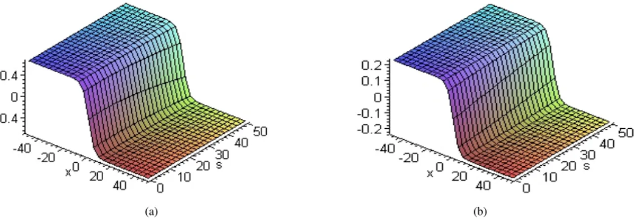
In order to check the efficiency of the VIM method for the equation (5.1), we draw figures for the numerical solution with𝛼 = 0.5 as well as the exact solution (5.3). Figure (a) stands for the numerical solution 𝑢₃(𝑡, 𝑥). Figure (b) shows the exact solution (5.3) when𝛼 = 𝛽 = 1. From these figures, we can appreciate how closely are the two solutions.

Remark 1 The Eq.(1) has been solved by ADM method in [2]. It should be remarked that the graph drawn here ( in the

case of time-fractional derivative) using the VIM method is agreement with the graph drawn using the ADM method.

4.2

Numerical Solutions of Space-Fractional Foam Drainage Equation

(a) (b)

Figure 1: Representing time fractional solutions of Eq.(5.1). In (a); solution obtained by the VIM method for𝛼 = 1₂. In (b); the exact solution (5.3);𝑐 = 0.02.

Assuming the condition as

𝑢(𝑥, 0) = 𝑓(𝑥) = 𝑥2_{. (5.7)}

Initial condition has been taken as the above polynomial to avoid heavy calculation of fractional differentiation. In order to estimate the numerical solution of equation (5.6), using the expression (4.8), we get:

𝑢𝑛+1(𝑥, 𝑡) = 𝑢𝑛− 𝑡 ∫ 0 [ 𝑢𝑛𝜏−1₂∼𝑢𝑛∼𝑢𝑛𝑥𝑥+ 2 (_∼ 𝑢𝑛 )2 𝐷𝛽 𝑥∼𝑢𝑛− ( 𝐷𝛽 𝑥∼𝑢𝑛 )2] 𝑑𝜏. (5.8)

By the iteration formula (5.8), we can obtain the other components as:

𝑢0(𝑥, 𝑡) = 𝑓(𝑥), 𝑢1(𝑥, 𝑡) = 𝑢0− 𝑡 ∫ 0 [ 𝑢0𝜏−12∼𝑢0∼𝑢0𝑥𝑥+ 2 (_∼ 𝑢0 )₂ 𝐷𝛽 𝑥∼𝑢0− ( 𝐷𝛽 𝑥∼𝑢0 )₂] 𝑑𝜏 = 𝑥2₊[_𝑥2_{− 4𝑓} 1𝑥6−𝛽+ 4𝑓12𝑥4−2𝛽 ] 𝑡, 𝑢2(𝑥, 𝑡) = 𝑢1− 𝑡 ∫ 0 [ 𝑢1𝜏−1₂∼𝑢1∼𝑢1𝑥𝑥+ 2 (_∼ 𝑢1 )2 𝐷𝛽 𝑥∼𝑢1− ( 𝐷𝛽 𝑥∼𝑢1 )2] 𝑑𝜏 = 𝑥2₊[_𝑥2_{− 4𝑓} 1𝑥6−𝛽+ 4𝑓12𝑥4−2𝛽 ] 𝑡 + [4𝑥2_{− 4𝑓} 1((6 − 𝛽) (5 − 𝛽) − 2) 𝑥6−𝛽 +4𝑓2 1((4 − 2𝛽) (3 − 2𝛽) + 2) 𝑥4−2𝛽− 2𝑥4 ( 2𝑓1𝑥2−𝛽+ 4𝑓1𝑓2𝑥6−2𝛽+ 4𝑓12𝑥4−3𝛽 ) −8𝑓1𝑥2−𝛽(𝑥4− 4𝑓1𝑥8−𝛽+ 4𝑓12𝑥6−2𝛽 ) + 4𝑓1𝑥2−𝛽(2𝑓1𝑥2−𝛽+ 4𝑓1𝑓2𝑥6−2𝛽+ 4𝑓12𝑓3𝑥4−3𝛽)]𝑡₄2 +[(𝑥2_{− 4𝑓1𝑥}6−𝛽_{+ 4𝑓}2 1𝑥4−2𝛽)(2 − 4𝑓1(6 − 𝛽) (5 − 𝛽) 𝑥4−𝛽+ 4𝑓12(4 − 2𝛽) (3 − 2𝛽) 𝑥2−2𝛽) −8𝑓1𝑥2−𝛽(𝑥2− 4𝑓1𝑥6−𝛽+ 4𝑓12𝑥4−2𝛽 )2_{− 8}(_{𝑥4− 4𝑓} 1𝑥8−𝛽+ 4𝑓12𝑥6−2𝛽 ) ( 2𝑓1𝑥2−𝛽+ 4𝑓1𝑓2𝑥6−2𝛽+ 4𝑓12𝑥4−3𝛽 ) + 2(2𝑓1𝑥2−𝛽+ 4𝑓1𝑓2𝑥6−2𝛽+ 4𝑓12𝑓3𝑥4−3𝛽)2]𝑡₆3 −2(𝑥2_{− 4𝑓} 1𝑥6−𝛽+ 4𝑓12𝑥4−2𝛽 )2(_2𝑓 1𝑥2−𝛽+ 4𝑓1𝑓2𝑥6−2𝛽+ 4𝑓12𝑥4−3𝛽 )_𝑡4 4. 𝑢3(𝑥, 𝑡) = 𝑢2− 𝑡 ∫ 0 [ 𝑢2𝜏−1₂∼𝑢2∼𝑢2𝑥𝑥+ 2 (_∼ 𝑢2 )2 𝐷𝛽 𝑥∼𝑢2− ( 𝐷𝛽 𝑥∼𝑢2 )2] 𝑑𝜏, (5.9)

and so on, in the same manner the rest of components of the iteration formula (5.8) can be obtained using the Mathe-matica Package.

Note that:

𝑓1= _{Γ (3 − 𝛽)}1 , 𝑓2=_{Γ (7 − 2𝛽)}Γ (7 − 𝛽) , 𝑓3=Γ (5 − 2𝛽)_{Γ (5 − 3𝛽)}. (5.10)

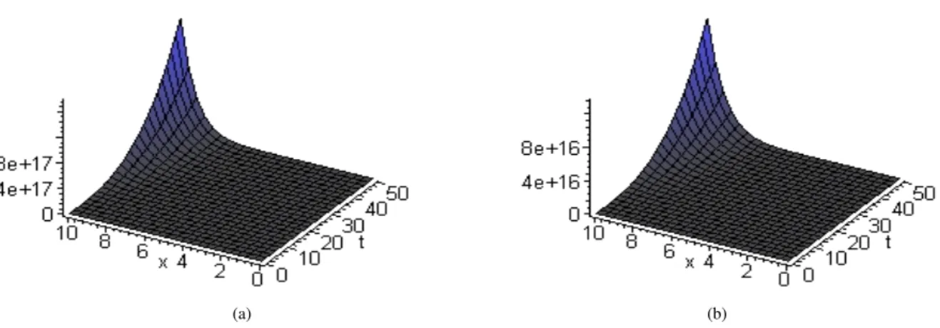
Figures (c,d) show respectively the numerical solution𝑢₃(𝑡, 𝑥) for the space-fractional Eq. (5.6) for 𝛽 = 1/2, respec-tively𝛽 = 1.

(a) (b)

Figure 2: Representing space-fractional solutions of Eq.(5.6). In (c); solution obtained by the VIM method for𝛽 = 1₂. In (d); solution obtained by the VIM method for𝛽 = 1.

Remark 2 : It should be remarked that the graph drawn here ( in the case of space fractional derivative) using the VIM

method is in excellent agreement with those drawn in [2] using the ADM method.

5

Conclusion

In this paper, the VIM has been successfully applied to derive explicit numerical solutions for the time-and space-fractional foam drainage equation. The main merits of the VIM are:

1. VIM can overcome difficulties arising in calculation of Adomian polynomials.

2. No linearization is needed; the method is very promising of finding wide application in nonlinear fractional evolu-tion equaevolu-tions.

References

[1] M.J. Ablowitz, P.A. Clarkson.Solitons, nonlinear evolution equations and inverse scatting. Cambridge University

Press, New York, (1991).

[2] Z. Dahmani, M. M. Mesmoudi, R. Bebbouchi. The foam-drainage equation with time and space fractional derivative solved by the ADM method. E. J. Qualitative Theory of Diff. Equ., 30:(2008), 1-10.

[3] Y. Chen, Y.Z. Yan. Weierstrass semi rational expansion method and new doubly periodic solutions of the generalized Hirota-Satsuma coupled KDV system. Applied Matheamtics and Computations, 177: (2006) ,85-91.

[4] M. Matinfar, A. Fereidoon, A. Aliasghartoyeh, M.Ghanbar. Variational Iteration Method for Solving Nonlinear WBK Equations. International Journal of Nonlinear Science , 8(4) :(2009).

[5] Qiaoxing Li , Jianmei Yang. Variational Iteration Decomposition Method for Solving Higher Dimensional Initial Boundary Value Problems Muhammad Aslam Noor, Syed Tauseef Mohyud-Din . International Journal of Nonlinear

Science, 7(1):(2009).

[6] J.H. He. Approximate solution of nonlinear differnetial equations with convolution product nonlinearities. Comput.

Methods. Appl. Mech. Engrg., 167 (1-2): (1998), 69-73.

[8] M.A. Helal, M.S. Mehanna.The tanh method and Adomian decomposition method for solving the foam drainage equation. Appl. Math. Comput., 190 :(2007) ,599-609.

[9] S. Hilgenfeldt, S.A. Koehler, H.A. Stone. Dynamics of coarsening foams: accelerated and self-limiting drainage.

Phys. Rev. Lett., 20 :(2001), 4704-7407.

[10] S. Kemple, H. Beyer. Global and causal solutions of fractional differential equations in : Transform Method and Special Functions. Varna96, Proceding of the 2nd International Worshop (SCTP), Singapore, (1997).

[11] Y. Luchko, R. Gorenflo. The initial value problem for some fractional differential equations with the Caputo derivaitve. Preprint Series A 08-98, Fachbereich Mathematik und Informatik, Freie Universitat Berlin, (1998). [12] A.M. Shahin, E.Ahmed, Yassmin A.Omar. On Fractional Order Quantum Mechanics. International Journal of

Non-linear Science, 8(4): (2009).

[13] I. Podlubny. Fractional Differential Equations. Academic Press, San Diego, (1999).

[14] G. Samko, A.A. Kilbas, O.I. Marichev. Fractional Integral and Derivative: Theory and Applications. Gordon and

Breach, Yverdon, (1993).

[15] G. Verbist, D. Weaire. Soluble model for foam drainage. Europhys. Lett., 26:(1994),631-634.

[16] G. Verbist, D. Weuire, A.M. Kraynik.The foam drainage equation. J. Phys. Condens. Matter, 8: (1996), 3715-3731. [17] Syed Tauseef Mohyud-Din, Ahmet Ytldtrtm. Variational Iteration Technique for Solving Initial and Boundary Value

Problems. International Journal of Nonlinear Science, 8(4): (2009).

[18] A. M. Wazwaz.The VIM method ofr rationel solutions for KdV, K(2,2) Burgers and cubic Boussinesq equations. J.

Comput. Appl. Math., 207 (1) :(2007), 18-23.

[19] B.J. Wesr, M. Bolognab, P. Grogolini. Physics of fractal operators.Springer, New York, (2003). [20] D. Weaire, S. Hutzler. The physic of foams. Oxford University Press, Oxford,( 2000).

[21] D. Weaire, S. Hutzler, S. Cox, M.D. Alonso, D. Drenckhan. The fluid dynmaics of foams. J. Phys. Condens. Matter, 15: (2003) ,65-72.