HAL Id: hal-02324431
https://hal.archives-ouvertes.fr/hal-02324431
Submitted on 26 Jun 2020
HAL is a multi-disciplinary open access
archive for the deposit and dissemination of
sci-entific research documents, whether they are
pub-lished or not. The documents may come from
teaching and research institutions in France or
abroad, or from public or private research centers.
L’archive ouverte pluridisciplinaire HAL, est
destinée au dépôt et à la diffusion de documents
scientifiques de niveau recherche, publiés ou non,
émanant des établissements d’enseignement et de
recherche français ou étrangers, des laboratoires
publics ou privés.
To cite this version:
A. Broquet, M. Wieczorek. The Gravitational Signature of Martian Volcanoes. Journal of Geophysical
Research. Planets, Wiley-Blackwell, 2019, 124 (8), pp.2054-2086. �10.1029/2019JE005959�.
�hal-02324431�
1Université Côte d'Azur, Observatoire de la Côte d'Azur, CNRS, Laboratoire Lagrange, France
Abstract
By modeling the elastic flexure of the Martian lithosphere under imposed loads, we provide a systematic study of the old and low-relief volcanoes (>3.2 Ga, 0.5 to 7.4 km) and the younger and larger prominent constructs within the Tharsis and Elysium provinces (<3 Ga, 5.8 to 21.9 km). We fit the theoretical gravitational signal to observations in order to place constraints on 18 volcanic structures. Inverted parameters include the bulk density of the load, the elastic thickness required to support the volcanic edifice at the time it was emplaced (Te), the heat flow, the volume of extruded lava, and the ratio of volcanic products that form within (Vi) and above the preexisting surface (Ve). The bulk density of the volcanic structures is found to have a mean value of 3, 206 ± 190 kg/m3, which is representative ofiron-rich basalts as sampled by the Martian basaltic meteorites. Tebeneath the small volcanoes is found to be small, less than 15 km, which implies that the lithosphere was weak and hot when these volcanoes formed. Conversely, most large volcanoes display higher values of Te, which is consistent with the bulk of their emplacement occurring later in geologic history, when the elastic lithosphere was colder and thicker. Our estimates for the volumes of volcanic edifices are about 10 times larger than those that neglect the flexure of the lithosphere. Constraints on the magnitude of subsurface loads imply that the ratio Vi∕Veis generally 3:5, which is smaller than for the Hawaiian volcanoes on Earth.
Plain Language Summary
The elastic deformation of the Martian lithosphere from volcanic edifices and magmatic intrusions was investigated for the old and low-relief volcanoes (>3.2 Ga, 0.5 to 7.4 km) and the younger and larger constructs clustered in the Tharsis and Elysium provinces (<3 Ga, 5.8 to 21.9 km). The observed topography is used to define the load and to derive a simulated gravity field that is compared to the observed gravity. The bulk density of the lava that composes all volcanoes is found to be 3,200 kg/m3, which is representative of iron-rich basalts as sampled by the Martian basaltic meteorites.The elastic part of the lithosphere, that is, the part maintaining loads over geologic time, is found to have been thin when the small, old volcanoes formed, which implies that the lithosphere was hot early in geologic history. Conversely, larger volcanoes are found to have been emplaced on a cold and thicker elastic lithosphere.
1. Introduction
Mars is believed to be in a stagnant lid regime where heat transport is dominated by diffusion through the lithosphere and by a weak advective motion in the mantle (Plesa et al., 2016). In this regime, the outermost part of the planet does not take part in mantle convection and crustal materials have not been recycled into the interior in any significant quantity since its formation. As a consequence, we witness, recorded in the crust and surface, the history of every geologic and geodynamic process that shaped the planet.
Because of the lack of plate tectonics on Mars, the primary magmatic extrusion mechanism is thought to be similar to hot spot volcanism on Earth. With no plate motion, this led to the formation of two broad volcanic provinces, Tharsis and Elysium with diameters of approximately 2,000 and 5,500 km, as well as more isolated edifices elsewhere such as Apollinaris Mons located near the equator with a diameter of 200 km. Recent evidence of volcanic activity dating from the last few tens of millions of years at calderas of large volcanoes suggests that Mars, despite its small size, was volcanically active over most, if not all, of its history (e.g., Hauber et al., 2011)
Studies of gravity and topography are one of the few methods that allow exploring in space and time the composition and thermomechanical properties of the crust-mantle system. Owing to the absence of surface recycling, the geodynamical responses of the planet to geologic loads are kept frozen within the mechanical memory of the lithosphere as the planet cools (Albert & Phillips, 2000). By investigating these time-invariant Key Points:
• The gravitational and topographic signature of Martian volcanoes as small as 200 km are investigated • The densities of the volcanic edifices
are constrained to be homogeneous with a mean value of3, 206 ± 190kg/m3
• The lithosphere is found to have been thinner beneath small, old highland volcanoes than the larger and younger Tharsis and Elysium volcanoes
Correspondence to:
A. Broquet,
adrien.broquet@oca.eu
Citation:
Broquet, A., & Wieczorek, M. A. (2019). The gravitational signature of Martian volcanoes. Journal of Geophysical Research: Planets, 124. https://doi.org/10.1029/2019JE005959
Received 6 MAR 2019 Accepted 26 JUN 2019
Accepted article online 4 JUL 2019
©2019. American Geophysical Union. All Rights Reserved.
flexural imprints, it is possible to recover portions of the planet's thermomechanical evolution throughout geologic time, from the young polar ice caps (e.g., Phillips et al., 2008; Wieczorek, 2008) to the ancient Tharsis volcanic province (e.g., McGovern et al., 2002, 2004).
The principle of using gravity and topography to investigate the lithosphere is based on the hypothesis that, over geologic timescales, the Martian lithosphere behaves as an elastic shell overlaying an inviscid mantle that bends in the presence of loads (Turcotte et al., 1981). The deflection of the elastic lithosphere varies as a function of temperature-dependent elastic parameters, as well as the thickness and density of loads acting on and beneath the surface (Kraus, 1967). When the elastic shell is thin with respect to the wavelength of deformation and the elastic properties are isotropic (Beuthe, 2008), a linear relationship exists, here referred to as admittance, that relates the height of the surface load (such as a volcano or a polar ice cap) to its gravitational anomaly.
A few localized admittance studies have been applied to the red planet using gravity data and surface topog-raphy that have been refined over time. The best model for the shape of Mars comes from the Mars Orbiter Laser Altimeter (MOLA) that was onboard Mars Global Surveyor (MGS; Smith et al., 2001). Global gravity solutions have improved significantly over the past two decades as a result of the accumulation of tracking data from MGS, Mars Reconnaissance Orbiter (MRO), and Mars Odyssey. Notable previously used global gravity solutions include models developed to spherical harmonic degree 80 by Lemoine et al. (2001), 95 by Konopliv et al. (2006), and 110 by Konopliv et al. (2011). The spatial resolutions of these models increased from approximately 133, to 112, and finally 97 km.
From admittance investigations, McKenzie et al. (2002) inverted for the crustal density and elastic thickness at various large-scale locations including the two giant Tharsis and Elysium provinces whose signatures dominate the Martian gravity field. McGovern et al. (2002, 2004) and Belleguic et al. (2005) estimated the elastic thickness of the lithosphere, the heat flow, and the density of the surface topography of several broad volcanoes that superimpose the same regions. Using a similar approach and as a result of the favorable space-craft's orbit geometry providing good data resolution at the south pole, Zuber et al. (2007) and Wieczorek (2008) were able to constrain the same parameters for the load associated with the young south polar cap. Beuthe et al. (2012) proposed a two-stage loading model for the major volcanic constructs, where the elas-tic thickness and density varied with time. Finally, Grott and Wieczorek (2012) investigated a single small volcano that is located in the southern highlands, Tyrrhena Mons.
In general, these studies revealed that the bulk density of the large volcanoes is high, approximately 3, 200 ± 100 kg/m3(e.g., Belleguic et al., 2005). If one accounts for the presence of about 5% to 10%
poros-ity, these estimates compare favorably with the grain density estimated from Martian basaltic meteorites (3,100 to 3,600 kg/m3) and with mineralogical models based on the surface concentration of rock-forming
elements measured by orbital Gamma-Ray Spectrometer data (3,250 to 3,450 kg/m3; Baratoux et al., 2014).
Compared to terrestrial basalts, where the largest grain densities are about 3,000 kg/m3(Moore, 2001), the
dense Martian basalts are characterized by a high Fe/(Fe+Mg) ratio and low Al2O3concentrations (Nyquist et al., 2001). For the small Tyrrhena Mons volcano, investigated by Grott and Wieczorek (2012), a similar high bulk density was obtained. The elastic thicknesses were found to be high (Te> 50 km) for the large vol-canoes (Belleguic et al., 2005), but the exact values differ somewhat from studies using more recent gravity models (Beuthe et al., 2012). For Tyrrhena Mons, the authors constrained the underlying elastic plate to be significantly weaker (Te< 20 km). These observations are consistent with geologic investigations and crater counting studies that show that small volcanoes formed early when the lithosphere was presumably hot and thin (Robbins et al., 2011; Williams et al., 2009). Finally, the present-day elastic thickness at the south polar cap was found to be at least 102 km (Wieczorek, 2008). Similar results were obtained at the North Pole from analyses of radar data that constrained the flexure under the ice sheet load (Phillips et al., 2008). Together, these results tell us that the lithosphere cooled with time and is currently characterized by a low heat flow (Grott & Breuer, 2010).
Several aspects regarding Martian volcanic activity and lithospheric properties remain unknown. This is a result of the low spatial resolution of the gravity models that limited previous surveys to large volcanic struc-tures with diameters in excess of 500 km, all of which have young surface ages (Robbins et al., 2011). These studies were also restricted to the southern highlands and to the Tharsis and Elysium volcanic provinces, where the gravity is well constrained. One unresolved question is whether the range of bulk densities obtained for the large volcanoes is representative of other smaller, spatially scattered, and possibly older
con-structs (Robbins et al., 2011; Williams et al., 2009). A second question is how Te(and the related heat flow) varies as a function of both position and time. Lastly, the volumes of materials that form within and above the preexisting crust are important constraints on the planet's magmatic activity and evolution, but these depend strongly upon the amount of lithospheric flexure. MOLA topographic data gave estimates on the vol-ume of volcanic constructs (see Plescia, 2004), but it was shown by Grott and Wieczorek (2012) that, at least for Tyrrhena Mons, the MOLA estimation is about 10 times smaller than the actual load volume as a result of significant lithospheric deflection. Furthermore, based on terrestrial experience, we suspect that signifi-cant quantities of magmatic products might reside beneath the edifice in the preexisting crust (Crisp, 1984; White et al., 2006) but the importance of these magmatic intrusives has not yet been constrained for Mars. To elucidate these questions, we will make use of the recent and improved gravity field model constructed by Genova et al. (2016). This model, GMM3_120, is based on Doppler tracking data from the MGS, MRO, and Mars Odyssey spacecraft and is developed up to degree 120 (89-km resolution). Although we will concentrate our study on the GMM3_120 model, we will also test our results using the similar solutions of Konopliv et al. (2016) and Goossens et al. (2017) that were obtained using different data sets and constraints, hereafter denoted as JGMRO_120 and GMM3-GOOSSENS_120, respectively.
These degree 120 models are the first to be above the spectral resolution threshold that is necessary to inves-tigate the gravitational signature of many volcanoes with sizes between 200 and 500 km. Armed with these solutions, and coupled with MOLA measurements of the planet's shape, we provide a systematic study of small to large volcanoes, many of which reside outside of the previously studied regions, by investigating their localized gravity and topography spectra. Eighteen volcanic constructs are found to provide robust local constraints on the surface bulk density, the elastic thickness of the lithosphere, and the related heat flow at the time each of them formed. With knowledge of the elastic flexure, we provide estimates on the volume of the extruded volcanic load by integrating the topographic and flexural profiles. Following previous studies (e.g., Belleguic et al., 2005), we also estimate if internal loads, assumed to be in phase with the surface load, are present in the crust or mantle. From this, we determine the volume of the internal load, by fixing the density contrast to plausible values. Comparing the surface and subsurface load volumes, we estimate the ratio of materials that forms within and above the preexisting crust (the intracrustal to extracrustal ratio), a value that can be compared with some volcanic systems on Earth (Quane et al., 2000; Vidal & Bonneville, 2004).
The outline of this paper is as follows. First, we give a brief review of the mathematical formalism that is used in describing the spectral properties of the gravitational field and the topography. We describe how the localized admittance can be used to invert for local parameters, such as the load density, the elastic thickness, and the volume of magmatic products that formed within and above the preexisting crust. Next, we discuss how uncertainties on the model parameters are estimated. We conclude by comparing our results with those obtained from earlier estimates (Belleguic et al., 2005; Beuthe et al., 2012; McGovern et al., 2004), and also with 3-D thermal evolution models (Plesa et al., 2018) after converting the elastic strength to a heat flow, and evaluate the implications of these for the composition of the surface and volcanic history of the planet.
2. Modeling
Modeling the relationship between the gravitational field and topography is often most easily done in the spectral domain using spherical harmonics (for more details, see Wieczorek, 2015). The spherical harmon-ics are the natural set of orthogonal basis functions on the sphere and are useful when modeling data on curved small bodies like Mars, where Cartesian methods might be inappropriate. Any real square-integrable function, g, can be expressed as a linear combination of these functions as
g(𝜃, 𝜙) = ∞ ∑ l=0 l ∑ m=−l glmYlm(𝜃, 𝜙) (1)
where Ylmis the spherical harmonic function of degree l and order m, glmis the corresponding spherical harmonic expansion coefficient, and𝜃 and 𝜙 represent the position on the sphere in terms of colatitude and longitude. These functions are orthogonal over both degree and order where we employ the “4𝜋” normaliza-tion convennormaliza-tion that is common in geodesy. Using their orthogonality properties, we can compute a power spectrum, which defines how the strength of the function varies with spherical harmonic degrees. “Power”
is here considered to be the average of the squared signal, and for a given function g, the total power is given by 1 4𝜋 ∫𝜃,𝜙g 2(𝜃, 𝜙) sin 𝜃 d𝜃 d𝜙 = ∞ ∑ l=0 Sgg(l) (2) where Sgg(l) = l ∑ m=−l g2lm (3)
is referred to as the power spectrum. The cross-power spectrum of two functions, g and t, can be similarly computed as 1 4𝜋 ∫𝜃,𝜙t(𝜃, 𝜙)g(𝜃, 𝜙) sin 𝜃 d𝜃 d𝜙 = ∞ ∑ l=0 Stg(l) (4)
where Stgis defined as the cross-power spectrum.
The gravitational potential can also be expressed as the sum of spherical harmonic functions U(r) = GM r ∞ ∑ l=0 l ∑ m=−l (R 0 r )l ClmYlm(𝜃, 𝜙) (5)
where G is the gravitational constant, M is the mass of the object, and R0is the reference radius of the
spherical harmonic coefficients. The gravitational acceleration is the gradient of the potential, and we will here use the radial component where
g(r) =GM r2 ∞ ∑ l=0 l ∑ m=−l ( R0 r )l (l +1) ClmYlm(𝜃, 𝜙) (6)
The admittance function is defined by
Z(l) = Stg(l)
Stt(l) (7)
and describes how the amplitude of the gravity signal is related to the topography and will be expressed in terms of milligals per kilometer. Here Stgis the cross-power spectrum of the gravity field and topography and Sttthe power spectrum of the topography. Another ratio of power spectra is the spectral correlation that describes the phase relationship of the gravity field and topography
𝛾(l) = Stg(l) √
Stt(l)Sgg(l)
(8)
where Sggis the power spectrum of the gravity field. If one assumes that the gravity and topography should be perfectly correlated and that an observed nonunity correlation is a result of “noise,” the uncertainty of the admittance can be shown to be
𝜎2(l) =Sgg(l)
Stt(l)
1 −𝛾(l)2
2l (9)
It is noted that Sgg =S̄ḡg+Svv, where S̄ḡgand Svvare the noiseless gravity and noise power spectra. If the signal-to-noise ratio is defined as S̄ḡg∕Svv, it can be easily shown that the correlation will correspond to
𝛾 = 0.775 when the signal-to-noise ratio is 1.5. This value of 𝛾 = 0.775 will be used as a minimum threshold when analyzing localized admittance spectra (e.g., Grott & Wieczorek, 2012; Wieczorek, 2008).
The global admittance and correlation spectra are plotted in Figure 1 using the gravity solutions JGMRO_95, JGMRO_110, JGMRO_120, GMM3_120, and GMM3-GOOSSENS_120. Both the correlation and admittance are seen to decrease dramatically at the highest degrees, which is a reflection of the maximum spatial reso-lution of the models. From these plots, we can see that the JGMRO_95 model of Konopliv et al. (2006) that
Figure 1. Admittance (left) and correlation (right) spectra of the gravity field and topography of Mars using the gravity
solutions JGMRO_95 of Konopliv et al. (2006), JGMRO_110 of Konopliv et al. (2011), JGMRO_120 of Konopliv et al. (2016), GMM3_120 of Genova et al. (2016), and GMM3-GOOSSENS_120 of Goossens et al. (2017).
was employed in several previous studies is reliable globally to only about degree 65. The JGMRO_110 model of Konopliv et al. (2011) extended the resolution to degree 80, whereas the degree 120 models of Konopliv et al. (2016) and Genova et al. (2016) are reliable globally to about degree 90.
The GMM3-GOOSSENS_120 model of Goossens et al. (2017) was constructed using a different approach than the others. Whereas previous models have constrained the power spectrum of the gravity field to follow a Kaula rule (in order to damp noise in the inversions), this model constrained the gravity coefficients to follow that predicted from surface topography. As a result of this, both the correlation and admittance are high at the highest spherical harmonic degrees. This regularization approach is less conservative than the use of a Kaula power law regularization. Consequently, we will focus on and make use of the model of Genova et al. (2016) in our analysis and also test the model of Konopliv et al. (2016) and then investigate whether the model of Goossens et al. (2017) allows us to analyze localized admittances to higher degrees. 2.1. Geophysical Loading Model
The study of mechanisms by which nonhydrostatic relief is supported has provided important constraints on the outermost part of the planet's rheological parameters. The simple model of Airy isostasy postulates that mountains float with crustal roots over the dense mantle. A second model assumes that topographic loads are partially supported by elastic stresses in the lithosphere, where the amount of flexure depends upon the thickness of the elastic lithosphere (Turcotte et al., 1981; Beuthe, 2008). The flexure model used here computes the purely elastic deflection of the lithosphere resulting from loads on (such as a volcano or a polar ice cap) and beneath the surface (such as a magma chamber or a mantle plume). We assume that the effective elastic thickness (or rigidity) of the shell reflects the elastic state when the load formed and was subsequently “frozen” into the mechanical memory of the plate as the planet cooled (e.g., Albert & Phillips, 2000).
The essence of this approach consists of deriving a linear equation that links the predicted gravitational signal to the observed planetary shape (Turcotte et al., 1981; Wieczorek, 2015)
glm=Qltlm+vlm (10)
where glm, tlm, and vlmare, respectively, the radial gravity field, the topography, and the part of the grav-itational signal that the model fails to predict (the so-called isostatic anomaly; see Forsyth, 1985), here presumed to be a zero mean random process. Qlis a model-dependent linear transfer function that is assumed to be isotropic (i.e., independent of order m). Multiplying each side of this equation by tlm, summing over all m and taking the expectation, we find that the transfer function Qlis identical to the admittance Z(l) given by equation (7).
We describe in the appendix a derivation of Qlusing a first-order relationship between surface relief and predicted gravity and a model of thin elastic shells (Turcotte et al., 1981). We note that models with thick
Table 1
Constants Used in the Flexure Model and the Range of Investigated Inversion Parameters
Parameter Symbol Value Unit Mean planetary radius R 3,389.5 km Young's modulus E 100 GPa Poisson's ratio 𝜈 0.25 — Mantle density 𝜌m 3,500 kg/m3 Crustal density 𝜌c 2,800–3,300 kg/m3 Load density 𝜌l 2,800–3,400 kg/m3 Elastic thickness Te 0–200 km Crustal thickness Tc 20–110 km Load ratio L −0.95 to 0.89 —
elastic shells (e.g., Banerdt et al., 1982) and with a minimum stress definition of isostasy (Beuthe et al., 2016) can also be found in the literature, but these generally yield similar results as long as the investigated wavelength is several times greater than the elastic plate thickness (Zhong & Zuber, 2000), which is the case in this study. The model is nearly identical to Grott and Wieczorek (2012), where the surface load density is allowed to differ from that of the crust. We improve upon their model by giving a more correct formulation for the degree of compensation function ̄Cswhen the crustal and load density differ. The density difference was neglected by Grott and Wieczorek (2012) when computing equipotential surfaces, but it was considered later for the derivation of the admittance. In the end, their expression for the admittance is equivalent to ours but with a different mathematical formulation for the quantity ̄Cs(equation (B11)).
In our model, the lithospheric deflections are computed by making use of the first-order mass sheet approx-imation. Though these are not significantly affected by this assumption, the final computed gravity signal is. Therefore, after calculating the deflections of the surface, crust, and mantle, using our elastic model, we use a finite-amplitude formulation as a final step to compute the exact gravitational potential associated with each layer (Wieczorek & Phillips, 1998). These are computed at the same radius, summed, and the result is then expanded in spherical harmonics in order to recover the power spectra from which the admittance and spectral correlation are obtained (equations (7) and (8)).
The transfer function Qlcan be schematically written as
Ql=Ql(rloc, Te, Tc, 𝜌l, 𝜌c, 𝜌m, L, z, E, v) (11) where Qldepends upon the spherical harmonic degree l; the local planetary radius rloc(associated with each
volcano; see section 2.3); the thickness of the elastic shell Teand crust Tc; the surface load, crust, and mantle densities𝜌l,𝜌c,𝜌m; a subsurface loading parameter L; the depth of the subsurface load z; and the Young's modulus E and the Poisson's ratio𝜈 of the elastic plate. In the following models, we set 𝜌m, E, and𝜈 similar to previous admittance studies (see Table 1 and Mcgovern et al., 2002). We explore the parameter space where we systematically vary𝜌l, Te, and L and then also evaluate the influence of plausible variations in Tcand𝜌c (see Table 1 and section 3.1).
The loading parameter L that can vary with the spherical harmonic degree l and order m is defined to be Llm = 𝑓lm∕(||𝑓lm|| + 1), where flmis the ratio of subsurface to surface loads (see appendix). For simplicity, and following previous investigations (e.g., Belleguic et al., 2005; Beuthe et al., 2012; McGovern et al., 2002), we assume that both loads are perfectly in-phase and that L is isotropic and independent of wavelength (Llm=L). This assumption of in-phase loads should be appropriate for volcanic provinces, where subsurface loads are expected to lie beneath the topographic edifice and can be validated by analysis of the spectral correlation between the gravity and topography, which should be high.
Our loading model is illustrated in Figure 2. In the left image, we display the case that involves only surface loading (L = 0) and in the right two panels, we present the internal loading scenarios corresponding to positive and negative values of L. For the case where L> 0, subsurface and surface loads have the same sign and it is assumed that the added internal material is a positive density contrast located at 50-km depth. This can be regarded as an addition of dense materials, such as magmatic intrusions in the crust. For L< 0, a
Figure 2. Schematic view of the surface and internal loading scenarios, where rlocis used as the zero elevation
reference. (left) The surface loading model (L=0), where hs, g, and wsare, respectively, the surface topography profile, the predicted free-air gravity, and the deflection under the topographic load. (right) The two different internal loading scenarios for dense intracrustal loading (L> 0) and buoyant mantle loading (L< 0), where wzis the deflection generated by the loads. Note that the depth axis is discontinuous.
negative density contrast is defined to reside in the upper mantle at 150-km depth, where the largest amount of melting is expected (Breuer et al., 2016). This can represent either a positive temperature anomaly or a depleted layer resulting from the prior extraction of magma in the upper mantle. The dense crustal intrusion generates a downward deflection of the lithosphere, whereas the buoyant mantle load generates an upward deflection. The depths of the load have little impact on the computed lithospheric deflections but do affect the final gravity calculation. Nevertheless, to first order, the depth of the load trade-offs with the density contrast of the load (note that a different sign convention was used in the paper of Belleguic et al., 2005, and that these authors placed the mantle load at 250-km depth). The final total deflection is obtained by adding the deflections resulting from both surface and subsurface loads.
When L > 0, it is sometimes possible that the addition of a positive density contrast in the crust leads to a singularity in the admittance equation for a single spherical harmonic degree (this was also observed by McKenzie, 2003; Lowry & Zhong, 2003; Beuthe et al., 2012). What happens physically is that the flexure due to the positive density contrast perfectly compensates the surface load such that the residual topography is zero and the admittance is infinite at a given wavelength. This can be seen in equation (B20), where the denominator terms tend to zero as the internal load term approaches unity. In the study of Beuthe et al. (2012), the authors decided to not investigate the part of the model where L > 0 in order to avoid this problem.
Though this singularity in the admittance equations can pose a problem when analyzing solely the admit-tance, it can be avoided by also making use of the spectral correlation. In particular, we note that when the singularity is crossed (with increasing spherical harmonic degree), the spectral correlation is predicted to change sign, from 1 to −1 (or the inverse). When comparing our theoretical gravity models to the observa-tions, it is only necessary to ensure that the signs of the predicted and observed correlation are consistent, that is, always positive for the volcanoes investigated in this study. Model parameters that provide theoretical correlations that are negative or lower than the observations are inconsistent with our model assumptions and are simply ignored.
In Figure 3, we demonstrate how our admittance model depends upon key parameters for the case where subsurface loads are not included (L = 0). For simplicity, the gravitational attraction was here computed using the first-order mass sheet approximation. In the left panel, we set all parameters to constant values (with Te =70km) and vary the load density between values representative of icy materials similar to the south polar cap (𝜌l =1, 250 kg/m3) to a Martian basalt (𝜌l =3, 300 kg/m3). This plot shows that the load density determines the asymptotic value of the admittance at high degrees. In the right panel, we set the load
Figure 3. A series of theoretical admittances for a varying surface density (left, with Te=70km) and elastic thickness
(right, with𝜌l=2, 900kg/m3), with other parameters set to constant values (Table 1).
density to 2,900 kg/m3and vary the elastic thickness for weak (T
e=10km) to rigid plates (Te=150km). The elastic thickness determines the wavelength range over which loads are compensated and has a large effect on the longest wavelengths. When the elastic thickness is high, the admittance resembles that expected for perfectly uncompensated surface topography, which can be approximated by 2𝜋𝜌lG(i.e., the Cartesian Bouguer plate approximation).
2.2. Treatment of the Degrees 1 and 2 Topography
When computing loads acting on the lithosphere and the resulting lithospheric deflections, we must treat the degrees 1 and 2 signal separately. When in a center-of-mass coordinate system, the degree 1 terms of the gravitational potential coefficients are by definition zero. If the degree 1 topography were treated as a load, this would result in a nonzero degree 1 gravity term that would be inconsistent with the reference frame used to express the surface topography and gravity. We note that in the thin shell theory there is no deflection predicted for degree 1 loads (see equation (B4)): a degree 1 load would simply shift the center of mass with respect to the origin and this would be inconsistent with the reference frames used to express the observed gravity and topography models. Thus, we will make the assumption that the degree 1 topography is perfectly compensated by Airy isostasy, which ensures that the center of mass is at the origin of the reference frame. The degree 2 topography and gravity are mostly due to the hydrostatic flattening of the planet, which is generated by its rotation. When computing the lithospheric deflections, we assumed that the degree 2 and order 0 term (C20) of the topography is entirely a result of rotational flattening and set the C20 deflection
coefficient to zero. Once the deflection of the different interfaces is computed (without C20), we added this
relief to both the surface load-crust and crust-mantle interface. Although it has been shown that the Tharsis bulge may create a small nonhydrostatic contribution to the C20term (Zuber & Smith, 1997), removing either
90%or more of this term has no influence on the forthcoming results. 2.3. Data Localization
Lithospheric properties are expected to vary across the surface of a planet. For this reason, it is necessary to obtain reliable spectral estimates from data that are restricted to specific regions of interest. In practice, this is accomplished by multiplying the data by a localization window and expanding the localized function in spherical harmonics (for more details, see ; Wieczorek & Simons, 2005; 2007; Simons & Dahlen, 2006). In the spatial domain, the localization procedure is performed as
G(𝜃, 𝜙) = g(𝜃, 𝜙) h(𝜃, 𝜙) (12)
where g is the global function, h is the localization window, and G is the localized function. The localization window should be specially constructed to minimize both its spectral bandwidth (to limit smoothing in the spectral domain) and the signal arising from outside of the region of interest. For this, we use the spherical cap localization windows of Wieczorek and Simons (2005, 2007) that are obtained by solving an optimiza-tion problem. These funcoptimiza-tions are analogous to the Slepian funcoptimiza-tions that are commonly used in Cartesian analyses.
For a given value of the angular radius of the spherical cap,𝜃, we adjust the spectral bandwidth of the win-dow, Lw, such that more than 99% of the power of the best concentrated window is located in the region of interest. For these calculations, we use the software package shtools of Wieczorek and Meschede (2018), which allows us to construct these functions, rotate them to the region of interest, and to perform the spherical harmonic expansions and spectral analyses.
As emphasized by Wieczorek and Simons (2005, 2007), multiplying the data by a window causes the local-ized power spectrum to differ from its global signature. In the wavelength range l < Lwthe windowed spectral estimates are heavily biased by wavelengths that are greater than the window size, and the spec-trum cannot be interpreted for l> Ldata−Lw, where Ldatais the maximum spectral resolution of the data,
because the localized spectrum depends upon degrees that have a higher resolution than the input field. We also stress that all the localized spectral estimates in the band l ± Lware correlated. In practice, we will only analyze localized spectra between the limits Lwand Ldata−Lw, and Lwwill need to be chosen to be small enough in order to have a sufficient number of degrees to constrain our inversion parameters.
In this study, we will make use of the gravity model GMM3_120 that is developed up to degree Ldata=120
(Genova et al., 2016). The spatial resolution of this model is variable, as defined by the degree strength (see their Figure 6). We expect that this value, which ranges respectively from 85 in the north to 100 in the south, underestimates the local resolution of the gravity field at the major volcanoes because the gravity signature in these regions is much greater than the value predicted by the Kaula law. We will thus set the maximum resolution of the model to be the point where the windowed admittance and spectral correlation drastically decrease, which we interpret as being due to the Kaula law damping applied during the inversion of the gravity coefficients (as observed in Figure 1).
In our analysis, we fix the size of the localization window to entirely encompass the region of interest, that is, the load and the associated expected flexural signal of longer wavelength while excluding signals arising from neighboring geologic structures. In this region, we compute the mean local radius, rloc, as the local
radius weighted by the amplitude of the localization window (T00∕h00). We do not exclude the edifice when
computing the local radius. In fact, the local radius only impacts the upward or downward continuation of the gravity coefficients from the modeled interfaces and observed gravity field. As long as the model and data are computed at the same radius, the solution is not influenced.
We emphasize that the power of the window is concentrated in the center of the localization region. As one approaches the angular radius of the cap, the data become progressively downweighted, which applies to all studies based on the localization approaches of Simons et al. (1997) and Wieczorek and Simons (2005). Typical window sizes that will be used vary from angular radii of𝜃 = 15◦and 6◦, which correspond to diameters of 1,816 and 712 km and spectral bandwidths of Lw=17and 42.
2.4. Inversion Procedure and Error Estimation
Many methods have been used to determine the best fitting model parameters and their uncertainties. McKenzie et al. (2002) did not give any range of variation in his inversion parameter estimates. McGovern et al. (2002) rejected all solutions yielding root-mean-square (rms) misfits greater than 10 mGal/km, val-ues that in general exceed the largest formal errors on the observed admittance. Belleguic et al. (2005) used both the expectation of the chi-square function and a Bayesian marginal probability under the assumption that every inverted degree is independent. This assumption, however, is not entirely correct in a localized framework where every localized admittance degree is partially correlated with those in the band l ± Lw (see section 2.3). Wieczorek (2008) and Grott and Wieczorek (2012) calculated the uncertainties using a restrictive criterion that all models fitted the admittance spectrum everywhere within its 1-𝜎 uncertainties, a method that does not allow for statistical outliers (see section 4.3). Beuthe et al. (2012) rejected solutions whose misfits were above 1.5 times the minimum rms.
Analyzing lunar gravity data from the Gravity Recovery and Interior Laboratory (GRAIL) mission, Besserer et al. (2014) explicitly computed the expected chi-square distribution by estimating the power spectrum of the signal that is not predicted by the model, which was treated as uncorrelated noise. For this method, it was assumed that the localized spectral correlation corresponded to the global value, which was justified given the high spectral degrees employed in their inversions. In this study, we initially attempted to use the approach of Besserer et al. (2014) to quantify the model uncertainties. However, given the low spectral resolution of the Martian gravity field in comparison to the GRAIL gravity models, the localized spectral
Table 2
Volcano Name, Location, Age, Maximum Relief With Respect to the Surrounding Terrane (Plescia, 2004), Window Angular Radius, and the Spherical Harmonic Degree Range Used in the Inversions
Volcano Latitude Longitude Age (Ga) Relief (km) 𝜃 Lw lmin–lmax Elysium rise 25.00◦ 147.00◦ 3.17+0−0.19.58 12.6 15◦ 17 23–70 Olympus Mons 18.50◦ 226.00◦ 0.42+0.03
−0.03 21.9 15◦ 17 24–67
Arsia Mons −9.20◦ 239.50◦ 0.13−0+0.02.02 11.7 10◦ 26 32–72 Pavonis Mons (a) 0.90◦ 247.50◦ 0.86+0−0.17.17 8.4 10◦ 26 32–48 Pavonis Mons (b) 0.90◦ 247.50◦ 0.86+0−0.17.17 8.4 10◦ 26 48–82 Alba Mons (a) 40.30◦ 250.24◦ 3.02+0−0.32.91 5.8 15◦ 17 20–35 Alba Mons (b) 40.30◦ 250.24◦ 3.02+0−0.32.91 5.8 15◦ 17 63–84 Ascraeus Mons 11.48◦ 255.30◦ 1.06+0−0.05.05 14.9 10◦ 26 32–70 Peneus Patera −57.00◦ 50.00◦ 3.75+0.08 −0.24 1.0 6◦ 43 48–60 Amphitrites Patera −59.50◦ 63.00◦ 3.63−0+0.07.13 1.0 6◦ 42 48–67 Tyrrhena Mons −21.36◦ 106.53◦ 3.41−0+0.08.16 1.5 7◦ 37 46–66 Hecates Tholus 31.90◦ 150.12◦ 3.52+0−0.11.57 6.6 7◦ 37 41–62 Albor Tholus 18.00◦ 150.24◦ 3.53+0−0.07.13 4.2 7◦ 37 45–65 Apollinaris Mons −8.80◦ 174.40◦ 3.77−0+0.04.06 5.4 7◦ 37 51–75 Biblis Tholus 2.40◦ 233.00◦ 3.35+0−1.19.45 3.6 6◦ 43 50–70 Ulysses Patera 3.30◦ 243.00◦ 1.42+0−0.30.30 1.5 6◦ 43 48–70 Uranius Tholus 27.06◦ 260.80◦ 3.57+0−0.06.09 2.9 6◦ 43 54–70 Ceraunius Tholus 22.80◦ 260.85◦ 3.59+0.05 −0.08 6.6 6◦ 43 47–70 Uranius Mons 26.10◦ 268.80◦ 3.43+0−0.05.07 3.0 6◦ 43 48–70 Tharsis Tholus 13.24◦ 269.00◦ 3.24+0−0.17.62 7.4 7◦ 37 46–72
Note. Longitudes are given in degrees east. Age estimates are derived from crater statistics by Williams et al. (2009) and Robbins et al. (2011), where the oldest age is here quoted when several surfaces were dated for the same volcano. For Alba and Pavonis Montes two ranges of harmonic degrees are investigated.
correlation was found to be considerably biased by the localization procedure. It was thus not possible to invert for the global unbiased correlation.
We instead used a variant of the method employed by McGovern et al. (2002) and determined the best fitting parameters by using an rms misfit function where
rms (Te, 𝜌l, L) = √ √ √ √ √ 1 N lmax ∑ l=lmin [ Z(l) − Zth(l, T e, 𝜌l, L) ]2 (13)
Here, Zth and Z refer to the localized predicted and observed admittances, respectively, and N is the number of degrees used in the summation. We estimated the range of acceptable parameters based on the average uncertainty of the admittance over the degree range that was analyzed. In a localized framework, this value is computed as ̄𝜍 = √ √ √ √ √ 1 N lmax ∑ l=lmin 𝜍2(l) (14)
where𝜍2is the localized version of𝜎2given by equation (9). In practice,𝜍2is similar to, but generally smaller
than, the cutoff used by McGovern et al. (2002). We performed an exhaustive grid search over the 3-D param-eter space and dparam-etermined the 1-𝜎 bounds on these parameters using the criterion rms (Te, 𝜌l, L) < ̄𝜍. Note that we also performed 4-D parameter space investigations (though with a lower resolution) where we evaluated the influence of the crustal density and thickness (see section 3.1).
Figure 4. Equirectangular projection of Martian topography from the model MarsTopo2600 of Wieczorek (2015).
Circles correspond to the size of the localization windows associated with the old and low-relief (dashed lines) and younger large volcanoes (solid lines). The triangles correspond to volcanoes that were investigated but that did not yield satisfactory results.
For each model, we computed the theoretical localized spectral correlation. If the theoretical value were ever less than the observed value for a given set of model parameters (as discussed in section 2.1), the rms misfit was simply set to infinity. Finally, we emphasize that if a chi-square function was used to estimate the best fit model parameters (where the difference between model and observations is scaled by the observed correlation), the best fitting parameters would only be slightly different and within the range of uncertainties estimated by our approach that used the rms misfit.
3. Results
In this section, we provide the results of our inversions for both small and large volcanoes on Mars. We start with a detailed description of the modeling procedure using as an example the small isolated Apollinaris Mons volcano, which is located near the Martian dichotomy boundary between the Tharsis and Elysium provinces. New results are then given for the low-relief volcanoes, and we follow by providing inversion results for previously studied large shield volcanoes. Table 2 provides the location, age, the maximum relief and volume of the edifices with respect to the surrounding terrane, and the chosen parameters of the local-ization windows. The analysis regions are shown in map form in Figure 4, and the results are summarized in Table 3–5.
3.1. Modeling Procedure at Apollinaris Mons
Apollinaris Mons is a low-relief volcano, located near the dichotomy boundary, at 174.4◦E, 8.8◦S. This vol-canic edifice stands 5.4 km above the surrounding terrane and has a summit caldera that is 1.8 km deep (Plescia, 2004). According to Robbins et al. (2011), Apollinaris Mons displays one of the oldest calderas (comparable in age to the volcanoes near the southwest rim of Hellas in our study), dating back to about 3.77 billion years ago (Table 2) and was also one of the first volcanoes to die out as no posterior activity is observed. The volcanic structure generates a local positive free-air gravity anomaly that strongly correlates with its topography (see Figure 5). Given the short phase of volcanic activity, no subsequent thermal reset-ting of the lithosphere is expected to have occurred, and the flexure associated with the volcano was likely frozen into the lithosphere as the planet cooled.
In order to investigate this volcano, we used a localization window of angular radius𝜃 = 7◦, which corre-sponds to a diameter of 832 km and a spectral bandwidth of Lw=37(see Figures 4 and 5). The location and diameter of this window were chosen in order to reduce the influence of local features and to maximize the observed correlation. The localized admittance and correlation spectra were computed following the
proce-Table 3
Summary of Results for the 18 Volcanoes
𝜌l(kg/m3) Te(km)
Volcano L=0 L≠ 0 L=0 L≠ 0 L rmsbest(mGal) 𝜍(mGal km−1) Elysium 3, 320+20−20 3, 340+20−40 12−4+4 10+6−4 −0.01+0−0.02.02 2.51 2.99 Olympus 3, 140+20−50 <3,200 68+32−18 78+42−28 0.12+0−0.04.12 1.79 3.16 Arsia 3, 130+20−20 3, 350+50−240 2−2+2 20+4−20 −0.17+0−0.17.08 0.91 2.14 Pavonis (a) >3,300 >2,810 40+20−20 62+48−42 0.17+0−0.03.17 0.90 1.45 Pavonis (b) — 3, 010+50−50 — 2−0+8 0.06+0−0.03.03 1.25 1.33 Alba (a) — 2, 950+100−100 — 6−6+4 0.28+0−0.07.07 2.30 3.90 Alba (b) — 3, 340+10−140 — 60−10+10 0.22+0−0.03.03 2.51 5.39 Ascraeus 3, 310+20−20 3, 000+330−20 14−2+2 48+2−36 0.11+0−0.06.11 0.70 0.81 Peneus 2, 930+100−30 <3,030 0+6−0 14+4−14 0.12+0−0.02.14 2.91 4.65 Amphitrites 2, 920+100 −10 2, 990+80−80 14+0−10 4+10−4 0.07+0−0.00.10 0.72 2.66 Tyrrhena 3, 350+50−70 3, 120+280−220 10−10+10 12+28−12 0.07+0−0.33.27 3.98 12.46 Hecates 3, 150+140−70 3, 160+240−80 42−30+8 38+12−28 −0.03+0−0.06.37 1.51 2.33 Albor — >3,380 — 0+10 −0 −0.07+0−0.02.02 3.92 4.05 Apollinaris — 3, 230+100−50 — 28−8+20 0.06+0−0.04.04 1.71 2.75 Biblis 3, 080+20−280 3, 010+90−210 0−0+88 0+100−0 0.03+0−0.14.88 3.32 8.31 Ulysses 3, 040+70 −70 3, 360+40−390 98+102−68 40+160−20 −0.21+0−0.41.16 0.87 3.24 Uranius Tholus 3, 00+70−100 3, 270+100−300 12−12+18 12+18−12 0.01+0−0.20.20 4.24 9.56 Ceraunius 3, 210+50−50 2, 990+410−50 12−12+28 14+26−14 0.07+0−0.08.47 2.73 5.86 Uranius Mons — 2, 930+100−10 — 0−0+6 0.10+0−0.01.06 2.10 4.69 Tharsis — 3, 150+20−20 — 6−6+16 0.04+0−0.02.00 2.40 3.06
Note. A dash means no acceptable fit found.
dures described in section 2.1. Before calculating the admittance, the observed gravity field was downward continued from 3,396 km to the average radius of the analysis region (3,387 km).
To define the range of investigated harmonic degrees, we first determine at which degrees the global sig-nature of Tharsis influences the observed admittance. Previous studies have noted that the global signal of Tharsis has an important contribution up to spherical harmonic degree 6 (Belleguic et al., 2005; Zuber & Smith, 1997), 7 (Beuthe et al., 2012), 8 (Wieczorek & Zuber, 2004) or 9 (Grott & Wieczorek, 2012). Recog-nizing that it is somewhat subjective as to where the Tharsis signature becomes insignificant, we chose to initially use a lower cutoff of Lw+ 7, which is sufficient for most volcanoes (see Table 2). However, for this
Table 4
Analyses Providing Constraints on the Crustal Density and Thickness
Volcano 𝜌l(kg/m3) 𝜌c(kg/m3) Tc(km) Elysium 3, 340+20−40 3, 100 ± 100 > 70 Olympus <3,200 3, 050 ± 150 — Pavonis >2,810 3, 100 ± 100 60 ± 20 Alba 2, 950+100−100 3, 080 ± 200 50 ± 20 Ascraeus 3, 000+330−20 3, 000+150−100 — Peneus — — <84 Amphitrites — — >38 Apollinaris 3, 230+100−50 <3,150 <20 Uranius Mons — — 60 ± 30
Table 5
Maximum Curvature of the Plate, Derived as the Second-Order Spatial Derivative of the Deflection, Heat Flow, Volume of the Volcanic Edifice or Surface Load (Ve), and Volume of the Internal Load (Vi) and Best Fitting Ratio of Viand Vefor the Case Where the Internal Load Is Located in the Crust (L> 0)
Volcano K(10−7m−1) Heat flow (mW/m2) V
e(104km3) Vi(104km3) Vi∕Ve Elysium 0.7+0−0.1.3 69−19+80 3, 253+1−1,579,252 − − Olympus 1.1+17−0.8.6 17+3−12 4, 845+5−3,656,121 3, 458+4−2,121,360 2:3 Arsia 0.6+0−0.1.2 42+∞−8 546+44−146 − − Pavonis (a) 0.6+0−0.1.2 18+26−6 539+395−225 517+567−217 1:1 Pavonis (b) 1.0+0−0.1.2 > 80 704+109−155 225+38−53 1:3 Alba (a) 2.2+1−2.0.0 120+∞−56 2, 570+633−1,920 4, 035+992−3,021 3:2 Alba (b) 0.2+0−0.1.1 19−1+2 754+578−113 1, 441+1−155,061 2:1 Ascraeus 0.5+18−0.1.1 18−2+57 1, 291+805−374 798+640−250 2:3 Peneus 2.4+7−1.9.0 47+∞−23 79+241−32 53+168−23 2:3 Amphitrites 4.5+6−1.6.1 158+∞−127 103+44−34 38+18−14 1:3 Tyrrhena 0.5+1−0.0.1 73+∞−53 106+33−69 42+13−28 2:5 Hecates 0.4+1−0.8.2 23+74−5 76+87−17 — — Albor 2.8+0−0.8.1 > 60 167+0−31 — — Apollinaris 0.7+4−0.6.1 29+13−13 149+81−70 51+30−24 1:3 Biblis 4.4+1−4.5.1 > 9 69+17−50 11+3−8 3:20 Ulysses 1.8+4−1.4.7 18+30−14 38+10−6 − − Uranius Tholus 5.1+1−5.6.0 46+∞−28 28+52−16 2+3−1 1:20 Ceraunius 0.8+7−0.0.7 58+∞ −42 40 +151 −16 15 +64 −7 2:5 Uranius Mons 18.3+16−7.4.4 > 49 99+75−31 54+44−18 1:2 Tharsis 5.0+0−4.1.7 100+∞−70 145+21−17 32+5−4 1:5
Note. Infinite heat flows correspond to Te=0km.
volcano, the model fit was found to be extremely poor for degrees less than 51, so here we used only degrees greater or equal than Lw+14(see Figure 6). We suspect that the poor fit for the first 14◦is a result of this old volcano being located at the edge of the Martian dichotomy boundary. At this location, the crustal thickness and density could both vary considerably and affect the longest wavelengths of the admittance. An addi-tional long-wavelength signature that could bias the lowest degrees is the Medusa Fossae Formation, which surrounds Apollinaris Mons that likely has a lower bulk density than average and was emplaced later in time when the elastic thickness was larger (Ojha & Lewis, 2018).
The highest degree to be inverted is limited to a maximum degree of Ldata–Lw. However, as a result of the lateral variation in resolution of the gravity global field, as well as the use of a Kaula law when constructing the solution, the maximum effective degree of the model can be lower than Ldata. The choice of the maximum
value is somewhat subjective, and in choosing this value, we considered principally the degree where the localized correlation and admittance break slope and begin to decrease and also the degree strength map of Genova et al. (2016). For Apollinaris Mons, where the degree strength is 95, lmaxwould be 58. We emphasized
in section 2.3 that this value likely underestimates the true resolution near volcanic edifices with large gravity anomalies, and given that both the model fit to the observations diverge and the spectral correlation starts to decrease at degree 75 (see Figure 6), we instead set lmaxto degree 75.
We investigated Apollinaris Mons using several forward models that include values of𝜌lfrom 2,800 to 3,400 kg/m3,𝜌
cfrom 2,800 to 3,300 kg/m3, Tcfrom 20 to 80 km, and Tefrom 0 to 200 km. The loading param-eter, L, is bounded from −1 to 1. In all models, we set the mantle density and rheological parameters to the values indicated in Table 1, which were used in previous admittance studies.
In our first set of inversion, we fixed the crustal thickness to 50 km and the crustal density to 2,900 kg/m3.
Results for the inversion of𝜌l, Teand L are shown in Figure 6. The left panel displays the observed localized admittance and correlation spectra using the GMM3_120 model as well as two best fitting admittances with
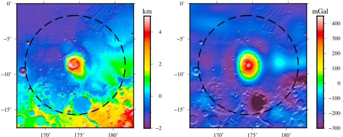
Figure 5. Topography and free-air gravity at Apollinaris Mons, both referenced to the average radius of the analysis
region (3,387 km). (left) Planetary shape model from MarsTopo2600 and (right) radial free-air gravity derived from GMM3_120, truncated at degree 110. The dashed circle indicates the location and size of the analysis region, here centered on the volcano and with a diameter of 832 km. The images are presented using a Lambert azimuthal equal area projection.
and without internal loading. The right panel of Figure 6 illustrates the minimum misfit as a function of𝜌l, Te, and L, where each value plotted represents the minimum misfit for all values of the other two parameters. When internal loads are neglected (L = 0), the best fit gives an rms misfit of 3.36 mGal/km, which is above our cutoff̄𝜍 of 2.75 mGal/km. Our best fitting model is for a surface load density of 3,230 kg/m3, an elastic
thickness of 28 km, and a subsurface load ratio of 0.06. The positive value of L indicates that the subsurface load is a result of dense materials located in the preexisting crust. The uncertainties on these parameters are approximately 75 kg/m3, 14 km, and 0.04 (see Table 3).
We performed similar inversions that included as a fourth free parameter either the thickness of the crust or the crustal density. For Apollinaris Mons, the crustal thickness model of Neumann et al. (2004) gives an average crustal thickness of 50 km, and we allowed the thickness at this site to vary from 20 to 80 km (e.g., Wieczorek & Zuber, 2004). When including the crustal density as a free parameter, we allowed this to vary from 2,800 to 3,300 kg/m3. For both of these inversions, the crustal thickness and density were not well
constrained, with all values larger than 20 km and smaller than 3,150 kg/m3being able to fit the data equally
well. The best fitting parameters of𝜌l, Te, and L did not change when including𝜌cor Tcas free parameters, but the uncertainties on𝜌land Teincreased by about a factor of 2.
The small amplitude of the internal crustal load, L = 0.06 ± 0.04, implies that the mass of the subsurface load is considerably smaller than the mass of the volcanic edifice, as might be expected for a low-relief construct. To assess the volume of magma that built the volcano, we performed a numerical integration of the surface topography and flexural profile associated with our best fitting results. For this calculation, we first set the global topography as a load acting on the lithosphere, with density and strength given by our best fits and investigated the local signal of the deflection. However, we noticed that the local deflection profile was affected by regional signals outside of the analysis region that are not associated with the volcano. An alternative approach was instead used where we performed a forward modeling of the deflection using the surface topography only within the analysis region. The local topography, referenced to the average radius at the edge of the region, was isolated in the spatial domain using a binary mask (tests using various forms of tapering were found to give the same results). When no deflection is considered, the volume of the surface load, Ve, is found to be 15 × 104km3. When lithospheric deflection is considered, we obtain volumes that are
about 10 times higher, equal to 149 × 104km3. By varying the elastic thickness and surface density within
their 1-𝜎 uncertainties, the uncertainty on the surface load volume is about a factor of 2.
The total volume of the load within the preexisting crust (the internal load) can be calculated using the definition of f from equation (B18), as Vi=f ×𝜌l×Ve∕𝛿𝜌, where f is the ratio of surface to subsurface loads and𝛿𝜌 is the density contrast of the intracrustal intrusion with respect to the surrounding crust. Setting 𝛿𝜌 equal to 400 kg/m3, the volume of the internal load is 51 × 104km3and is uncertain by the same factor of
2 as the surface load volume. From these, we determine the ratio of magmatic products within and above the preexisting crust: Vi∕Ve, where Viand Veare, respectively, the volumes of the internal and surface loads
Figure 6. Results for Apollinaris Mons. (left) Observed localized admittance and spectral correlation using GMM3_120, best fitting predicted admittances with
L=0and L=0.06, with thermsbestmisfit in milligals per kilometer. Red dots represent the range that is investigated. (right) Misfit curves as a function of𝜌l,
Te, and L. The horizontal solid line represents the acceptable misfit,̄𝜍.
and are found to be about 1:3 (see Table 5). By varying𝜌l, Te, and L within their 1-𝜎 uncertainties, the ratio
Vi∕Veis found to vary from 1:9 to 3:5. We emphasize that the ratio of magmatic products within and above the preexisting crust differs from the intrusive to extrusive ratio defined by Crisp (1984) and White et al. (2006). In these studies, subsurface magmatic materials located in the volcanic edifice would be treated as intrusives, whereas our study would consider them to be part of the surface load and hence part of the volume of materials located above the preexisting crust.
Finally, to test whether our small localization window correctly captures the flexural signature of the volcano and if our analysis is sensitive to reasonable variations in the analysis parameters, we performed several inversions with larger window sizes and different degree ranges. These analyses included window sizes with angular radii from 6◦to 10◦, values of lminfrom 38 to 57, and values of lmaxfrom 59 to 86. We always obtained similar results, with best fitting parameters within the given error bars. The uncertainties were also found to be comparable, although we note that slightly higher uncertainties are obtained when a smaller range of degrees is investigated.
3.2. Low-Relief Volcanoes
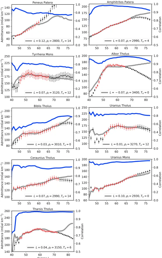
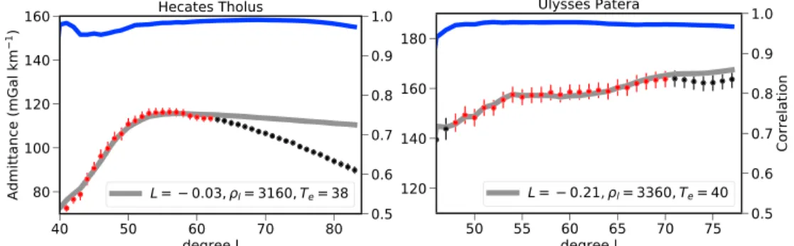
In this subsection, we investigate 11 old small volcanoes with ages that are generally greater than 3 Ga (Ulysses Patera is an exception with an age as young as 1.42 Ga, being the only age reported in Robbins et al., 2011). Inversions were performed for𝜌l, Te, and L, with Tcand𝜌cfixed to 50 km and 2,900 kg/m3. We present below nine small volcanoes that have small elastic thicknesses including Peneus Patera, Amphitrites Patera, Tyrrhena Mons, Albor Tholus, Biblis Tholus, Uranius Tholus, Ceraunius Tholus, Tharsis Tholus, and Uranius Mons and two with larger elastic thicknesses, Hecates Tholus and Ulysses Patera. Best fitting results and uncertainties are given in Table 3, and the best fitting admittance spectra are presented in Figures 7 and 8. As with Apollinaris Mons, we also varied the angular radius of the localization window, as well as the
Figure 7. Localized admittance, correlation, and best fitting theoretical admittance spectra for the small and old
Figure 8. Localized admittance, correlation, and best fitting theoretical admittance spectra for the two small volcanoes
with high elastic thicknesses. Figures are plotted in a similar manner as Figure 6.
lminand lmaxbounds for each volcano, and found that this did not significantly impact the results presented
below.
At the southern rim of the Hellas impact basin reside six of the oldest volcanoes on Mars that are thought to have formed quickly after the impact event, between 4.0 and 3.6 Ga (Williams et al., 2009). Among them, three were found to have a correlation high enough over a robust range of harmonic degrees to be inves-tigated, namely, Pityusa Patera, Peneus Patera, and Amphitrites Patera. Although Pityusa Patera satisfies these two criteria, its gravitational signature is not successfully modeled by our simple loading model in that no set of values within the parameter space can reproduce the observed admittance signal. For Peneus and Amphitrites Paterae, our elastic flexure model yields a satisfactory fit to the data with an elastic thickness of 14 (+4, −14) km. The loading parameter of these two volcanoes is 0.07 (+0.0, −0.10) and 0.12 (+0.02, −0.14), indicating the presence of dense crustal intrusives. The load densities are similar for both edifices, about 2, 900 ± 100 kg/m3, which is considerably lower than that of the other volcanoes in our study. We next
per-formed inversions including either Tcor𝜌cas a fourth free parameter (see Table 1). For Amphitrites Patera, the crustal thickness was constrained to be larger than 38 km with a best fit at 70 km, and for Peneus Patera, we found that all values below 84 km could fit the observations, with a best fit equal to 54 km (see Table 4 and Figure A1). For both volcanoes, the best fitting values of𝜌l, Te, and L did not vary when Tcwas allowed to vary but the uncertainties increased by at most a factor 2. The crustal density was not constrained for either edifice, and including this parameter in our inversion increased the uncertainties by about 30%. Tyrrhena Mons is a small central vent volcano, located in the southern highlands, east of the Hellas Basin (see Figure 4), which was investigated previously by Grott and Wieczorek (2012) using the JGMRO_110 gravity model. Owing to the better-resolved field of Genova et al. (2016) that increases the correlation at higher degrees (see Figure 1), we were able to investigate Tyrrhena Mons using 10 additional spherical har-monic degrees in comparison to their study. The admittance is well fitted with any elastic thickness below 20 km and with a high load density of about 3, 350 ± 60 kg/m3was obtained when internal loading is not
considered. A small improvement of the model fit to the data is obtained when crustal loads are consid-ered, L = 0.07 (+0.33, −0.27), with 𝜌l = 3, 120 (+280, −220) kg/m3and T
e = 12(+28, −12) km. Our best fitting parameters compare favorably with those of Grott and Wieczorek (2012), and the uncertainties are improved by a factor 2.
Albor Tholus is superposed on the Elysium rise, which is itself a much larger volcanic construct (see Figure 4). For this volcano, the bulk density of the load is found to be higher than 3,380 kg/m3and the
litho-sphere is constrained to be weak with an elastic thickness below 10 km. The subsurface loading parameter is found to be −0.07 ± 0.02, which favors the presence of a small buoyant load in the underlying mantle. Given that this volcano is superposed on the Elysium rise, it is conceivable that the magnitude of the subsur-face load is biased by that associated with the larger Elysium rise, which is likely fed by a long-lived mantle plume.
Biblis Tholus lies on the western portion of the Tharsis plateau, which is a volcanic province that covers up to one fourth of the planet's surface. Twelve shield volcanoes of different size (>200 km), extent, and morphology are found in this region. Biblis Tholus is considerably smaller than the largest volcanoes in this province but is older with an age of 3.35 (+0.19, −1.45) Ga (Robbins et al., 2011). For Biblis Tholus the best