Design and Analysis of Wearable Conductive Fiber Sensors for Continuous Multi-Axis Joint Angle Measurements
by Peter T. Gibbs B.S. Mechanical Engineering The Ohio State University, 2003
Submitted to the Department of Mechanical Engineering in Partial Fulfillment of the Requirement for the Degree of
Master of Science in Mechanical Engineering at the
Massachusetts Institute of Technology February 2005
0 2005 Massachusetts Institute of Technology All rights reserved
Signature of A uthor... ... Department of Mechanical Engineering
December 14, 2004
C ertified by...
A ccepted by... Chairma
Xiaruhiko Harry Asada Ford Professor of Mechanical Engineering Thesis Supervisor
Professor Lallit Anand n, Department Committee on Graduate Students
MASSACHUSETTS INSTWE'i OF TECHNOLOGY
Design and Analysis of Wearable Conductive Fiber Sensors for Continuous Multi-Axis Joint Angle Measurements
by Peter T. Gibbs
Submitted to the Department of Mechanical Engineering on January 14, 2005 in Partial Fulfillment of the Requirements for the degree of Master of Science in
Mechanical Engineering
Abstract
The practice of continuous, long-term monitoring of human joint motion is one that finds many applications, especially in the medical and rehabilitation fields. There is currently a lack of acceptable devices available to perform such measurements in an accurate and non-intrusive way for a patient over a long period of time, and so a new wearable sensor has been developed. A novel technique of incorporating conductive fibers into flexible, skin-tight fabrics surrounding a joint is used. Resistance changes across these conductive fibers are measured, and directly related to specific single or multi-axis joint angles through the use of a nonlinear predictor after an initial, one-time calibration. These wearable sensors are comfortable, and acceptable for long-term wear in everyday settings. Because these sensors are intended for multiple uses, an automated registration algorithm has been devised using a sensitivity template matched to an array of sensors spanning the joints of interest. In this way, a sensor array can be taken off and put back on an individual for multiple uses, with the sensors automatically calibrating themselves each time. Results have shown the feasibility of this type of sensor, with accurate measurements of joint motion for both a single-axis knee joint and a double axis hip joint when compared to a standard goniometer used to measure joint angles.
Thesis Supervisor: Haruhiko H. Asada Title: Professor of Mechanical Engineering
ACKNOWLEDGMENTS Dedicated to my family, my parents, and my wife, Carla.
A special thank you to Professor Harry Asada for his guidance, support, and kindness in my time at MIT.
TABLE OF CONTENTS
1 Introduction... 7
1.1 M otivation... 7
1.2 Existing M ethods of M easuring Hum an M ovem ent... 8
1.3 Proposal and Overview ... 9
2 M easurem ent Principle and Sensor Design ... 11
2.1 W orking Principle... 11
2.2 Predictor D esign ... 13
2.3 M isalignm ent and M ulti-Thread Design... 18
3 Sensor Registration ... 20
3.1 M ulti-Thread Sensor Arrays ... 20
3.2 Registration Algorithm ... 23
3.2.1 Single-Axis Case... 23
3.2.2 Double-Axis Case ... 26
3.3 M odel Sim ulations ... 29
4 Experim ental D esign and Im plem entation... 35
4.1 W earable Joint M easurem ent Garm ent... 35
4.1.1 Sensor Pants for Lower Body M onitoring ... 36
4.1.2 Conductive Fiber Characteristics... 37
4.2 Prelim inary Experim ents ... 38
4.3 Single-Axis Joint Angle M easurem ent Results ... 40
4.4 M ulti-Axis Joint Angle M easurem ent Results... 46
5 Conclusion ... 50
5.1 Discussion... 50
5.2 Sum m ary of Contributions... 52
6 Appendix... 53
6.1 Silver Plated N ylon Characteristics ... 53
LIST OF FIGURES
Figure 2-1: When a joint such as the elbow bends, fabric surrounding the joint will
contract or extend to a new length. ... 11
Figure 2-2: Schematic of sensor design. This particular arrangement shows one sensor running lengthwise across a single-axis knee joint... 13
Figure 2-3 Three sensors used to measure three lower body joint angles. ... 14
Figure 2-4: Preliminary data showing sensor output vs. knee flexion angle... 14
Figure 3-1: (a) Array of equidistantly spaced sensors over knee joint. (b) Array shifted by an unknow n distance, a... 20
Figure 3-2 (a) Array of equidistantly spaced sensors over knee joint, with each sensor having unique sensitivity in this calibration position. (b) Shifting of array by an unknown distance, a, will lead to a shift in sensitivities... 22
Figure 3-3 Block diagram of single array sensor operation... 25
Figure 3-4 Schematic of two sensor arrays in a pair of pants to measure hip angles. (a) side view , and (b) rear view ... 27
Figure 3-5 Schematic of average sensitivities of two arrays of two joint angles. Proper registration of array 1 assured only if Y, >> a, and Y2 (F 2<< -2---... 28
Figure 3-6 Schematic of knee model used in simulations. ... 29
Figure 3-7 Sensitivity curves for 5 sensor array in calibration position (solid, y*), and offset from calibration position (dashed, y) by an angle a/r=13 ... 30
Figure 3-8 Sensitivity plots for 5-sensor array shifted by a1/r=13' from calibration. New sensitivities are approximately shifted versions of the calibrated sensitivities... 31
Figure 3-9 Function to be minimized, Rj(n), for a 5-sensor array offset by aj/r=13' (y(i)=00, 15', 300, 450, 600)... 32
Figure 3-10 Function to be minimized for multiple offsets of a symmetrically calibrated 9-sensor array (with y(i)=-20', -15', -10', -5', 0, 5', 100, 15, 200)... 33
Figure 3-11 Error in estimation of Oj(3) when y(i) = 0', 10', 200, ... , 60 . ... 34
Figure 3-12 Error in estimation of Oj(3) when y(i) 0', 4', 80, ... , 60 . ... 34
Figure 4-1 Spandex pants with conductive fiber sensors for lower body monitoring ... 36
Figure 4-2 Measurements were taken from a standard electrogoniometer at Position 1 (00) and Position 2 (500)... 38
Figure 4-3 Sensor Output vs. Knee Joint Angle for three sensor threads... 39
Figure 4-4 Comparison of goniometer measured knee joint angle and estimated angles from w earable conductive fiber sensor. ... 41
Figure 4-5 Joint Angle Estimations for Various Frequencies of Joint Motion... 42
Figure 4-6 Joint Angle Measurements with Sensing Garment taken off and put back on b efore each test ... . . 45
Figure 4-7 Hip sensor outputs for two distinct leg motions... 46
Figure 4-8 Comparison of goniometer measured hip joint angles and estimated angles from wearable conductive fiber sensors: (a) Hip Flexion/Extension, (b) Hip A bduction/A dduction... 48
LIST OF TABLES
Table 4-1 Conductive Fiber Characteristics (~100 denier fibers)... 37 Table 4-2 Fiber Sensor Errors for Various Frequencies of Joint Motion ... 43 Table 4-3 Estimating knee joint angle of 90' with and without registration algorithm... 44 Table 4-4 Fiber Sensor Errors for successive tests where pants have been taken off and
p u t b ack o n ... 4 5
1
Introduction
1.1
Motivation
Long-term ambulatory measurement of human movement is an important need in the medical field today [1]. For many types of rehabilitation treatment, it is desired to monitor a patient's activities of daily life continuously in the home environment, outside the artificial environment of a laboratory or doctor's office [2]. This type of monitoring is quite beneficial to the therapist, allowing a better assessment of human motor control, and tremor or functional use of a body segment, over long periods of time [1]. Evaluating a patient's daily life activities allows a more sufficient assessment of a patient's disabilities, and aids in developing rehabilitation treatments and programs, as well as assessing a treatment's effectiveness [2,3]. In addition, the recognition of deviations in joint movement patterns is essential for rehabilitation specialists to select and implement an appropriate rehabilitation protocol for an individual [4,5].
Many specific medical applications clearly benefit from the information provided by continuous human movement monitoring. To better develop and optimize total joint replacements, for instance, a detailed record of a patient's daily activities after such a replacement is required [6]. The measurement of tremor and motor activity in neurological patients has long been studied [7]. In pulmonary patients, it is often desired to precisely quantify the amount of walking and exercise performed during daily living, since this is a fundamental goal in improving physical functioning and life quality [3]. Furthermore, physiological responses, such as changes in heart rate or blood pressure,
often result from changes in body position or activity, making the assessment of posture and motion an essential issue in any type of continuous, ambulatory monitoring [8].
1.2 Existing Methods of Measuring Human Movement
Presently, there exists no single, satisfactory solution to the problem of measuring human movement on a continuous basis. The use of video and optical motion analysis systems offer the most precise evaluation of human motion, but obviously restrict measurements to a finite volume [9]. Body mounted sensors such as accelerometers or pedometers are frequently used for monitoring daily physical activity, but are often limited in the reliable information they are able to provide [3,7]. Even methods of self-report designed to gather information on general daily activity, such as diaries or questionnaires, are time consuming and often unreliable, especially for the elderly relying on their memory [3].
Electrogoniometers are frequently used to measure dynamic, multi-axis joint angle changes in individuals, providing continuous joint movement information. These devices do not completely satisfy conditions desired for monitoring activities of daily living, though, since they are exoskeletal devices that cross the joint, potentially interfering with movement. Furthermore, any shift from their original placement leads to errors in angle estimations [2]. Such commercially available goniometers can produce erratic readings once the device is detached from the patient body and put back on the same joint in a slightly different orientation. It is therefore difficult to use these goniometers at home for long periods of time.
The idea of an entirely wearable device to detect human motion is not a completely new concept. Specialized goniometric devices have been constructed for specific wearable applications using traditional techniques, including instrumented gloves [10-13], but are often relatively cumbersome, and not easy to attach to the body permanently. Various other types of textile fabrics with integrated sensing devices have also been devised [14, 15]. In each of these cases, though, the sensing devices are typically traditional strain gauges, carefully attached to an article of clothing. One patented device uses conductive fabrics acting as strain gauges on a garment to emit "effects" such as light or sound based upon a wearer's movements [16]. While this is a novel wearable device, it is not designed, nor is suitable, for long-term accurate joint angle measurement.
For all types of body-mounted sensors, the issues of comfort and wearability are of major importance, since a patient will be wearing the monitoring device for extended periods of time. Furthermore, such home-use wearable sensors need to be put on and off every day without close supervision of a medical professional. Proper registration of the sensor is therefore a crucial requirement for deploying wearable sensors to the home environment.
1.3 Proposal and Overview
The goal of this thesis is therefore to develop a new method for continuous monitoring of human movement by measuring single or multi-axis joint angles with a wearable sensing garment that is non-intrusive and non-cumbersome and that can be properly registered for reliable monitoring. A new method is presented here for joint monitoring using conductive fibers incorporated into comfortable, flexible fabrics. All
that is needed is a one-time manual calibration with a standard goniometer, and a conductive fiber sensor garment is then able to continuously detect joint movement and measure specific single or multi-axis joint angles. With an array of sensors incorporated into a sensing garment, registration of the sensor occurs automatically each time the garment is worn through only a few simple motions by the wearer. This type of wearable sensor would allow extended home monitoring of a patient, and is no harder to put on than a typical article of clothing.
In the following, the design details and working principles behind this wearable device will be presented, as well as the algorithms developed that allow truly continuous monitoring. Results will also be shown from the implementation of these sensors on both single-axis and multi-axis joints.
2 Measurement Principle and Sensor Design
2.1 Working Principle
Figure 2-1 shows the basic principle behind a wearable sensor that measures joint movement. When a particular joint moves, skin around the joint stretches, along with any form-fitting fabric surrounding the joint as well. A former study by the textile industry has shown that body movements about joints require specific amounts of skin extension. Lengthwise across the knee for example, the skin stretches anywhere from
35-45% during normal joint movement [17].
Figure 2-1: When a joint such as the elbow bends, fabric surrounding the joint will contract or extend to a new length.
When a particular joint moves, fabric around the joint will either expand or contract accordingly, assuming the fabric is form fitting to the skin, and has the necessary elastic properties. For stretch sufficient to provide comfort and freedom of body movement, stretchability of 25 to 30 percent is recommended for fabrics fitting closely to the body
[17]. By incorporating conductive fibers into such a fabric surrounding a joint, the conductive materials will necessarily change length with joint movement. The electrical resistance of the conductive material will change as well, and can be directly measured
and correlated to changes in the orientation of the joint.
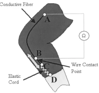
Fig. 2-2 shows how a single conductive fiber is implemented as a sensor. One end of the conductive fiber is permanently attached to the nonconductive, form-fitting fabric substrate at point A in the figure. The other end of the conductive fiber, point C, is kept in tension by a coupled elastic cord, which is permanently attached to the remote side of the joint, point D. Therefore, any stretching in this coupled material will take place in the highly elastic cord, CD, and not in the conductive fiber AC. As the joint moves, the elastic cord will change length, causing the coupled conductive fiber to freely slide past a wire contact point at B that is stationary (permanently stitched into the fabric). The conductive fiber always keeps an electrical contact with this wire, but the length of conductive thread between points A and B will change as the joint rotates. The resistance, which is linearly related to length, is then measured continuously across these two points A and B.
Conductive Fiber
0
Wire Contact Point ElasticD CordFigure 2-2: Schematic of sensor design. This particular arrangement shows one sensor running lengthwise across a single-axis knee joint.
2.2 Predictor Design
Consider Fig. 2-3. Shown here are a sensor spanning across a single axis knee joint, and a pair of sensors about a double axis hip joint. The angles of interest are labeled 01,
62, and 63. Our goal is to estimate these joint angles based upon the output of sensors 1, 2, and 3.
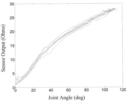
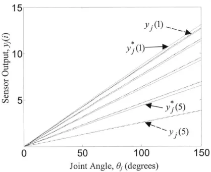
Preliminary experiments have shown a clear relationship between joint angle and sensor output for individual sensors about various joints of the body. Fig. 2-4, for instance, shows a typical set of output data from a single sensor thread across a single-axis knee joint with the output "zeroed" for a joint angle of 0'.
3
Figure 2-3 Three sensors used to measure three lower body joint angles.
30 25 S20 15 10-5 / 0 20 40 60 80 100 120
Joint Angle (deg)
It is desired to design a filter that receives sensor signals as inputs, and predicts the joint angle(s) of interest. In the proposed method, each joint angle being monitored has a
corresponding single sensor that is situated about that particular joint for maximum sensitivity, as in Fig. 2-3.
Consider N axis sensors for measuring N joints, each consisting of a single thread sensor, as shown in Fig. 2-3. The simplest predictor model that can be used is a linear regression:
o= G y+0
0 (2.1)where 0=( .. - N is the N x l vector of N joint angle predictions, O is its bias
term, y = (y ... YN ) is the N x 1 vector of corresponding sensor readings, and G and
O are, respectively, the N x N matrix and the N x 1 vector experimentally determined to relate the inputs and the outputs.
Since there is a slight amount of curvature in the preliminary data of Fig. 2-4, a nonlinear predictor may be more effective. We will use a second order polynomial model
0 =0 0+Gy+G'y' (2.2)
where
(y y2 ... yN-N (3)
and G' is an N x N(N-1)/2 experimentally determined matrix. The three terms on the right hand side of the above equation can be incorporated into a single term using augmented matrix and vector:
0= WY (2.4)
where W and Y are
W =
(0
0 G G') ''1 Y = y 'y (2.5) (2.6)To determine the parameter matrix W, a least squares regression is performed using
m sets of experimental data from a collection of sensors on an individual patient. Let P
be a N x m matrix consisting of m sets of experimentally measured joint angles,
0 (1)
L
N
N)(2.7)
and B be a {1+N(N+1)/2} x m matrix their quadratic terms:
containing the corresponding sensor outputs and
(2.8)
The optimal regression coefficient matrix W* that minimizes the squared prediction errors is given by
W* = PBT (BBT) 1 (2.9)
if the data are rich enough to make the matrix product BBT non-singular.
The above expressions are the most general forms for N axis sensors. In practice, however, they can be reduced to a compact expression with lower orders. First the offset 00 can be eliminated from the coefficient matrix W, if the sensor outputs are zeroed at a particular posture, e.g. the one where the extremities are fully extended. Second, although the matrix G contains off-diagonal elements representing cross couplings among multiple joints, some joints have no cross coupling with other joints. For example, the knee joint is isolated and has apparently no correlation with the hip joints. If the j-th joint is decoupled from all others, it can be treated separately as:
Oi
= (g g (2.10)where the offset is eliminated. Third, although multiple joints are coupled to each other having non-zero off-diagonal terms in matrix G, their cross coupling can be a limited one with proper design of individual sensors, so that their second order coupling may be negligible. In such a case, two coupled joints, sayj and k, can be written as:
0j 911 912 9'11 9'12 S21 Ak (2.11)2.1
k x g91 2 2 g'21 g'2 2)Y
where the offset terms have been eliminated. Thus the number of parameters to identify through calibration experiments is reduced. In consequence, the dimension of the optimal coefficient matrix must be reduced accordingly. The same calibration procedure is performed for both single axis and multiple axis cases, and need be performed only once for a specific set of sensors on an individual.
2.3 Misalignment and Multi-Thread Design
The orientation and pattern of the conductive fibers in the nonconductive fabric is the major design consideration. For a single-axis joint, one sensor is sufficient to capture the joint's motion. For multi-d.o.f. joints, though, multiple conductive fibers are needed to measure the multiple angles created.
For a single sensor spanning a joint, the ends of the sensor are located at points in the material that are remote from the joint. In this way, these points are relatively stationary for normal joint movement, and all length change due to fabric extension occurs between these points. The location of these points should be chosen such that the maximum dynamic range of sensor extension is utilized for maximum sensitivity to a particular joint angle change. For example, one sensor running lengthwise across the knee joint as shown in Fig. 2-2 is sufficient to provide sensor outputs with excellent sensitivity to knee flexion angle.
Although one sensor is sufficient to capture single-axis joint motion, any misalignment of such a sensor from use to use will lead to erroneous measurements. From a practical standpoint, it is obvious that a method is needed to adjust for any shifting of a sensor about the joint that will take place from one use to the next. It is both undesirable and impractical to recalibrate a sensor for each and every use. To take care of such registration problems, an array of multiple sensor threads is used. By incorporating multiple threads in a known pattern, a template-matching algorithm can be performed to determine a sensor's offset from calibration. In this way, measurement errors due to sensor misalignment are significantly reduced. The details of this method are described in the next section.
3 Sensor Registration
3.1 Multi-Thread Sensor Arrays
The goal in designing this wearable sensor is to create a device that is ultimately self-registering for subsequent uses after the initial one-time calibration experiments. This means that no additional equipment is needed to register the sensors for each use. Also, it is important that any procedures that are needed for self-registration are simple, and able to be preformed by the patient without supervision. To achieve these goals, a multi-thread sensor array design is presented.
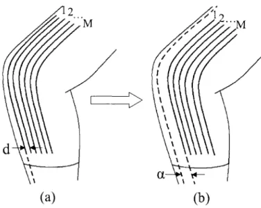
First, consider an array of M sensors covering a single-axis joint as shown in Fig. 3-1(a).
2 ...M
I ) \
d
(a)
(b)
Figure 3-1: (a) Array of equidistantly spaced sensors over knee joint. (b) Array shifted by an unknown distance, a.
Each sensor thread is separated from the adjacent sensor thread by a known, constant distance, d. This multi-thread sensor array is used to estimate a single-axis joint angle, O;. To develop a registration procedure let us first calibrate each sensor thread individually. Let 0 (i) be the estimate of the j-th joint based on the i-th thread sensor given by
0j(i) = Hj(i)Y (i) (3.1)
where
'y1(i)
Y(i) = 2 (3.2)
y
y(i))and Hj (i) is the 1 x 2 regression vector that is optimized for the i-th single-thread sensor of the j-th joint placed at a home position.
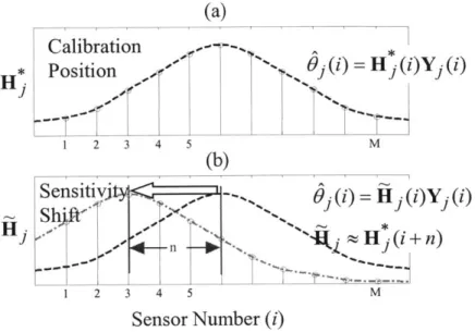
Now consider the situation where the sensor array has been removed, and placed back on the joint for more measurements. The sensor array is now offset an unknown distance, a, from the home position where calibration was performed. See Fig. 3-1(b). Since the individual single-thread sensors in the array are equally spaced, each sensor thread is shifted from its home calibration position by the same distance a. Assuming that the individual sensor threads are identical other than being separated by a distance d, we can conclude that the pattern of the sensitivity array is a shifted version of the calibrated one, as shown in the simplified plots of Fig. 3-2. This reduces the self-registration problem to a type of pattern matching problem.
Calibra * Positio H
1
1 2 (a) tion--n O (i) = H1(i)Yj (i)
3 4 5 (b) M Sensitivjty
S
-' -n 1 2 3 4 5-Oj
(i)
=H
j(i)Y1 (i)H (iM n)
M
Sensor Number (i)
Figure 3-2 (a) Array of equidistantly spaced sensors over knee joint, with each sensor having unique sensitivity in this calibration position. (b) Shifting of array by
an unknown distance, a, will lead to a shift in sensitivities.
H j (i) will no longer be the appropriate regression matrix to estimate 6O from Y1(i) .
A new, unknown vector Hj (i) will instead relate the sensor output to O:
01(i) = H j(i)Y1(i) (3.3)
Although H1 (i) is unknown, each individual sensor in the array should ideally give the same estimate for the actual joint angle at any time, so that
01 = Hj()Y(1) = Hj(2)Y1(2) =-= (M)Y,(M). (3.4)
If the shifting of the sensor array were to happen in a discrete fashion,
a = nd (3.5)
where n is an integer value, it is seen that
(i) = H*(i+n) (3.6)
Since n is an unknown, it is desired to find an n that satisfies (3.4) and (3.6), rewritten as
H (1+ n)Yj (1) = H* (2+ n )Yj (2)== H* (M)Yj (M - n ), if n O 0. (3.7a)
H j ()Yj (1+|n|) = H*) (2)Yj (2+|n|) =- - (M - n|)Yj (M), if n < 0. (3.7b)
In the ideal, theoretical case, there will exist an integer n that can be found to exactly solve (3.7). Unfortunately, for practical usage, n will not be a discrete integer. Furthermore, n will not be able to be explicitly found since process and measurement noise will cause the sensor outputs to deviate from their "ideal" values. With the knowledge of H j(i) for M discrete positions, though, it is possible to find the optimal integer n that best solves (3.7).
3.2 Registration Algorithm
3.2.1 Single-Axis Case
Let us first define the average joint angle estimate for M threads of sensor outputs for a given integer n as follows (with Y and H* reducing to scalars for the linear case):
I M-Inj
Oj (n) - I H (i+ n )Y (i), for n 0. (3.8a)
M- n
Oj (n) = 1 I H1 (i)Yj (i + n ), for n <0. (3.8b)
M - jn =
The best estimate for n is found by minimizing the average squared error between each sensor's estimate and the average estimate with respect to n (i.e. reducing the
variance in the estimated angle as a function of n):
I M - nj 2
Rj (n > 0) = -Hj I (i + n )Yj (i) -- O (n)) (3.9a)
M - nn 2= M -n ~ iy~ + -
( .b
Rj (n < 0) = HI (i)Y1 (i+ n) - O (n)) (3.9b)nj
= arg min R1 (n) (3.9c) nEquations (3.9a) and (3.9b) are solved for n = -M+2, -M+3, ... , M-3, M-2. The value for 57 found from (3.9c) is then used in (3.6) to approximate each sensor's predictor regression matrix for this new offset position of the array. In the ideal discrete case, where a=nod, no is the discrete offset of the sensor array,
n1
= no, and Rj (ni )= 0.For the non-ideal case, where a is not a discrete multiple of d, Rj (nj) # 0, but will approach zero as M increases, and d decreases. Creating a denser sensor array in this way leads to more accurate estimations of sensor sensitivities, which in turn leads to
using this algorithm, a one-time calibration is all that is needed for these wearable sensors to be used by a patient.
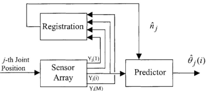
The registration algorithm takes place in real time as the sensor is in use. While registration is not needed at all times, it should be performed during initial operation until an appropriate n1i is converged upon. Again, the denser the array of sensors used, the better the estimate obtained. Following this, the algorithm need not be performed as often, since the sensor array should remain fairly stationary for an individual use. To begin monitoring, it is assumed that h =0. Fig. 3-3 shows a simplified block diagram of the process.
Registration n
j-th Joint YM O) $7(i)
Posiin-0 Sensor -- o. Predictor
10 Array Yi
Yj(M)
Figure 3-3 Block diagram of single array sensor operation.
All that is needed for a patient to begin using these sensors it to first "zero" the sensor output with the joint fully extended in the 0' position, and then freely move the joint to obtain non-zero data. This non-zero data will then allow the self-registration to take place.
3.2.2 Double-Axis Case
In the double axis case, two sensor arrays are placed around a predominantly two-axis joint such as the hip. As in the single-axis case, each array contains M sensors equally spaced by a distance d. The j-th array is placed so that it is most sensitive to changes in
O;, while the k-th array is situated so that it is most sensitive to changes in 64. Using the quadratic model, (2.11) can now be written as:
y1(i) *. Yk()
Oki1) G jk (i,1) 2 (3.10)
Yk (1)2
for the i-th and /-th sensor threads in thej-th and k-th sensor arrays respectively, and
G*k(i,) --
r
11 912 g'11 g'12 (3.11) g21 922 g'2 1 g'22 (The sensor arrays are placed in the wearable garment such that g11 and g22 are the
dominant terms in the G jk (i, 1) matrix.
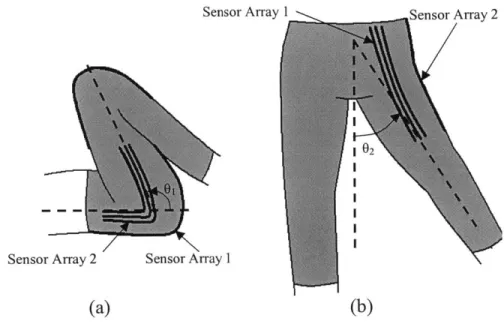
Fig. 3-4 shows a schematic of a pair of pants with two sensor arrays used to measure both hip flexion/extension (01) and hip abduction/adduction (62).
Sensor Array 1 -.
Sensor Array 2 Sensor Array 1
(a) (b)
Figure 3-4 Schematic of two sensor arrays in a pair of pants to measure hip angles. (a) side view, and (b) rear view
To use the registration algorithm developed for the single-axis case, it is necessary to break the two-axis motion of the joint into two single axis measurements. Since each sensor contains information from both joint angles, it is desired to perform the registration algorithm when only one axis of the joint motion is "activating" the sensors. Furthermore, in looking at Fig. 3-4, a shifting of one sensor array in the horizontal direction will be accompanied by a nearly identical shift in the second array. Therefore, registering one array will also register the other. For this reason, it is required that a patient performs only one simple movement when first putting on the sensors - extending the joint about a single axis over a "suitable" range.
By initially varying only 01, for example, it is known that 02 = 0 . Since the sensor threads in array 1 are most sensitive to changes in 01, and the sensor threads in array 2
terms in (3.11) except g, I and g1i . The problem is therefore reduced to a single axis registration. In this way, both sensor arrays can be registered, without any knowledge of the true joint angle.
To verify that a patient has indeed extended his or her joint over a "suitable" range for proper registration, an additional test can be performed to verify the motion is usable for registration. Consider Fig. 3-5. When the average sensor output from sensor array 1 (yi) is above a certain threshold (ai), and the average sensor output from sensor array 2
(Y2) is below another threshold (G2), it can be deduced that the primary joint motion is
due to changes in 01 alone. In this case, sensor array 1 can then be registered as in the single axis case. If these conditions are not met, then the patient has not necessarily moved his or her joints over a wide enough range to ensure proper registration.
0 0L
2-3.3 Model Simulations
To illustrate the registration concepts just discussed, consider the single-axis model knee joint of Fig. 3-6.
d
i+1
01 M
ri
Figure 3-6 Schematic of knee model used in simulations.
The change in length of the i-th sensor is modeled by the equation
yj (i,01, aO )= rj01 cos r(i) + a1 (3.12)
Sri
where r is the radius of the joint (note that for the following simulations, r is a constant of 5 cm), and y(i) is the angular position of the i-th sensor from the centerline ("calibration") position. When aj = 0, there is no sensor misregistration, and the sensors
are therefore in the calibration position. In this particular model, Oj is linearly related to yj(i), and therefore g'= 0 in (2.10).
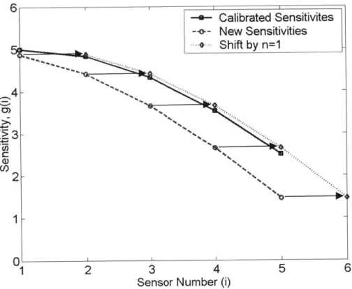
First, let us consider a 5-sensor array with y(l) = 0*, y(2) = 15', y(3) = 300, y(4)= 450, and y(5) = 600. The solid lines in Fig. 3-7 show the resulting calibration curves from the
sensors in these positions from (3.12) with a1 = 0. Now consider the same array with the sensors shifted by a1/r = 13'. The dashed lines of Fig. 3-7 show the new curves for the
sensors in such an arrangement. Obviously these differ significantly from the calibrated curves. Furthermore, these new curves would be unknown in a real application where a is unknown. 15 y1 (1) 10 ... y1 (5)
0
50
100
150
Joint Angle, Oj (degrees)
Figure 3-7 Sensitivity curves for 5 sensor array in calibration position (solid, y*), and offset from calibration position (dashed, y) by an angle a/rj=13'
Fig. 3-8 shows the same data as Fig. 3-7, except that here, the sensitivities are plotted for each sensor thread in both its calibration position, and its new, "unknown" position. It is easier to see in Fig. 3-8 that the new sensitivities are approximately a shifted version
of the calibrated sensitivities. Specifically, shifting the new sensitivity curve by n=1 gives the best approximation of the calibrated sensitivity curve, as shown.
-- Calibrated Sensitivites
-o- New Sensitivities
Shiftby
n=
2 3 4
Sensor Number (i)
5 6
Figure 3-8 Sensitivity plots for 5-sensor array shifted by a/r;=13' from calibration. New sensitivities are approximately shifted versions of the calibrated sensitivities
To find the necessary shift for a real application (where the new sensitivity curve is unknown), we implement (3.9). Fig. 3-9 shows Rj plotted vs. n for this situation. As
expected, the minimum value of Rj(n) occurs at n=1. 6 4 f4-4 >3 C) 2 1 - 0-1
0.1 0.08 Minimized at 0.06 / 0.04 0.02 -3 -2 -1 0 1 2 3 Discrete Offset, n
Figure 3-9 Function to be minimized, Rj(n), for a 5-sensor array offset by a/r;=13*
(y(i)=0 , 150, 300, 450, 600).
Now consider a 9-sensor array using this model, with y(l) = -20', y(2) = 15, y(3)=
-100,..., y(8) = 15', and y(9) = 200. In this case, the discrete spacing between sensors is 5'. Fig. 3-10 shows Rj plotted vs. n for various offset conditions of this array. Four different
sensor offsets were simulated: a;/r; = 00, 50, 120, and 14*. As expected, the resulting minimum values for Rj occurred at n = 0, 1, 2, and 3 respectively. For the case where
a;/r; = 120, the Rj values at n = 2 and n = 3 are fairly close, which could lead to ambiguity
in a real sensor application. This is due to the fact that "12"' falls almost right in the middle of 100 and 150, the corresponding sensor calibration positions for n=2 and n=3.
0.015 c = 0 deg E = 5 deg x = 12 deg 0.01 a = 14 deg 0.005 0 -5 -4 -3 -2 -1 0 1 2 3 4 5 Discrete Offset, n
Figure 3-10 Function to be minimized for multiple offsets of a symmetrically
calibrated 9-sensor array (with y(i)=-20', -15', -10', -5', 0', 50, 100, 150, 20')
Figures 3-11 and 3-12 show simulated errors in the estimated joint angle, Oi (3), for a single sensor thread (thread 3) in an array as a function of array offset, a;. In Fig. 3-12, the simulated sensors were more densely spaced than in Fig. 3-11. The figures show results from before the registration algorithm is implemented, and after the registration algorithm is implemented. In comparing these two plots, it is seen that as the sensor spacing decreases, estimation errors decrease as well. Furthermore, it is seen that this is an effective way to significantly decrease measurement errors. For example, without the registration algorithm, measurement errors are as great as 20% in the case of Fig. 3-12. Implementing the registration algorithm, the maximum theoretical error is reduced to less than 3%.
4j 35 30 25 20 15 10 5 0 10 30
Sensor array offset, a (degrees)
Figure 3-11 Error in estimation of O;(3) when y(i) = 00, 100, 200, ..., 60'.
40 25 20 15 10 5 0 0 Before Registra After Registratictionn
A A
10
Aa
20 30
Sensor array offset, a (degrees)
Figure 3-12 Error in estimation of O;(3) when y(i) = 00, 40, 8 , ... , 600.
-a--- Before Registration
-e---- After Registration a a
A A a a a / ~ a A a a a a 0A3 ~a, a a ~K a' 0
4 Experimental Design and Implementation
4.1 Wearable Joint Measurement Garment
Another important goal in producing a joint measurement garment is to design for
wearability. While it is difficult to produce quantitative measures of such a subjective
parameter as wearability, attempts have been made to produce design guidelines for wearability. One such set of considerations necessary for the design of wearable products is outlined below [18]:
" Placement (where on body product will go) * Form/shape of product
* Human movement considerations " Sizing (for body diversity) * Attachment to body " Weight of product
* Thermal issues (must allow body to breathe) * Aesthetics
* Long term use
Taking all these principles into account, it is ultimately necessary that a wearable device is comfortable, unobtrusive, and does not hinder normal body movement in any way. Along with sensor functionality, these were the issues considered when designing the wearable joint movement sensor garment described in the following section.
4.1.1 Sensor Pants for Lower Body Monitoring
Fig. 4-1 shows a prototype pair of spandex pants with conductive fibers incorporated into the fabric to measure lower body movement.
Figure 4-1 Spandex pants with conductive fiber sensors for lower body monitoring
Spandex was chosen due to its favorable qualities: very stretchable, elastic, fits closely to the skin, and is able to withstand normal body movements and return to its original shape with no permanent distortions [17]. Furthermore, it is a comfortable material, able to be worn on a daily basis since it does not restrict movement in any way. Thus it is quite suitable for this sensor design.
In these particular pants, an array of eleven sensors spans across the knee joint, each separated by a distance of 5 mm, and each with an unstretched length of 55 cm. Single sensors span both the posterior and side of the hip as well to capture two axes of hip motion. These single sensors are not seen in the view of Fig. 4-1, but the locations are the same as those shown for sensors 1 and 2 in the schematic of Fig. 2-3. This is the sensing garment used for all experimental tests summarized in the following sections.
4.1.2 Conductive Fiber Characteristics
In choosing a particular type of conductive fiber to incorporate into the wearable sensing garment, conductivity and durability were the properties of most concern. Shown in Table 4-1 are four types of commercially available conductive fibers, and their respective properties. From the analysis of these properties, silver plated nylon 66 yarn was ultimately chosen for implementation in the sensing garment due to its relatively low impedance properties and high strength. Specific characteristics of the exact fibers used in the sensor pants are presented in section 6.1 of the Appendix.
Table 4-1 Conductive Fiber Characteristics (-100 denier fibers)
Name Resistance (fl/cm) Elongation at Break (%)
Resistat ® (carbon sulfide >104 30-35
bonded to nylon fibers) Thunderon @ (copper
sulfide bonded to nylon 102-103 25-30
fibers)
X-Static ® (silver based <101 25-30
fiber)
4.2
Preliminary Experiments
This research has been conducted under a protocol approved by the Massachusetts Institute of Technology Committee on the Use of Humans as Experimental Subjects (Approval No. 0411000960).
To get an idea of the capabilities of existing technology available for joint monitoring, tests were initially performed using a standard electrogoniometer. This was a BIOPAC TSD130B Twin Axis Goniometer that consisted of two telescoping end-blocks that were taped to the side of the leg on either side of the knee joint. A strain gauge between these blocks was the device that measured the joint angle. The goniometer was used to measure knee flexion angle for two discrete positions as shown in the schematic of Fig. 4-2. An untrained professional attached the goniometer to the leg, but followed the recommended attachment procedures as described by the vendor in the instruction manual. This was to simulate the knowledge of a typical patient who would be using
such a device on his or her own, outside a carefully controlled setting.
Figure 4-2 Measurements were taken from a standard electrogoniometer at Position 1 (00) and Position 2 (500)
The goniometer was taken off and placed back on the knee joint eight separate times. Each time the goniometer was put on, the leg was extended and the goniometer output
was set to 00. The leg was then bent to Position 2 (500) and the goniometer output was recorded. The average rms error between the goniometer output, and the known joint angle (50') for these tests was 3.5* with a standard deviation of 2.6'. Even with the goniometer placed on the same joint by the same person, these results illustrate the fact that slight changes in how the goniometer is attached can lead to varying measurements. It will be important to keep errors such as these in mind when the results from the conductive fiber sensor are analyzed in the following sections.
Having just discussed the possible errors introduced by a standard electrogoniometer, it is important to also highlight the possible errors introduced by a conductive fiber thread sensor. Consider Fig. 4-3, which shows sensor output vs. knee flexion angle for three different thread sensors on the pants garment when the knee was randomly swung over a large range of motion.
30 25- 20-151 10 a . A: . ---0 20 40 60 80 100 120
As can be seen from this figure, there is a significant amount of variation possible in sensor output for a given joint angle. In particular, for these particular threads, the average rms error between these curves, and the calibrated predictor curves from (2.10) was approximately 30-50 over the many tests performed. Therefore, it is noted upfront that errors will be introduced based solely on the type of measuring device being used due to hysteresis, material uncertainties, and other processes that cannot be accurately modeled. This should be kept in mind when using such a wearable device.
4.3 Single-Axis Joint Angle Measurement Results
The pants sensing garment was first used to estimate single-axis knee angle measurements. For the following single-axis experiments, a rotary potentiometer firmly attached to the leg was used as a goniometer, and this was the standard for which to compare joint angles. In each experiment, the potentiometer was "zeroed" with the leg in the full extension position.
A calibration was performed to find the optimal regression matrix for both the linear and nonlinear predictors, and a sequence of knee movements was then monitored with the sensors. Fig. 4-4 shows the results of a typical sequence of these knee measurements, comparing the estimated angle from the conductive fiber sensors using the predictor models to that of the rotary potentiometer firmly attached to the leg.
-- Potentiometer Output
---- Linear Model Estimation -- Quadratic Model Estimation
8 0 '~60-20 0 0 4 8 12 16 20 Time (sec)
Figure 4-4 Comparison of goniometer measured knee joint angle and estimated angles from wearable conductive fiber sensor.
The performance of the pants sensors can be seen to be quite good, accurately capturing the joint movement patterns over time. The average rms error between the pants sensor estimate and the potentiometer using the linear predictor was 5.4', while that
for the quadratic predictor was significantly better, at just 3.20.
It is important that these sensors are able to measure all types of motion, including higher frequency motion. To determine the frequency capabilities of the prototype fiber sensors, tests were performed where the leg was swung back and forth at different frequencies. The resulting sensor estimations, and errors when compared to the potentiometer, are summarized in Fig. 4-5 and Table 4-2 respectively.
-0.1 Hz
1c
Cd
90 - - , - - - , - - -
-- Potentiometer Output
80 Fiber Sensor Output
70 60 ?o\ 80. ~0.. 30 20 2 36 40 44 48 52 Time (sec) -0.5 Hz to , - - - , -.- --. - , --.-.-.- . .- --.. .. -.-.. . -. . - Potentiometer Output
Fiber Sensor Output
to. 60 to. 20-,0. 60 61 62 63 64 65 66 Time (sec) -1 Hz 9 0 - - - -- - - -- - - ~ -Potentiometer Output Fiber Sensor Output
80-70 0 <40 -30Z Al 20 10 - -Tf ( Time (see) 80 70 50 40 90 80 70 40 30 20' 76.4 -2 Hz I Potentiometer Output
Fber Sensor Output
-t
79.8 80 80.2 80.4 80.6
Time (sec) 80.8 81 81.2
-1.5 Hz
Potentiometer Output Fiber Sensor Output
76.8 77.2
Time (sec)
Figure 4-5 Joint Angle Estimations for Various Frequencies of Joint Motion
77.6 78
:41 V
Table 4-2 Fiber Sensor Errors for Various Frequencies of Joint Motion Approximate Average RMS Error
Frequency (Hz) (degrees) 0.1 3.8 0.5 6.6 1 5.5 1.5 4.9 2 7.1
From these results, it is seen that the sensors are able to track the joint motion for frequencies as high as 2 Hz, but significantly larger errors result as the frequency is increased. Since most gross human motion takes place below these frequencies in a typical day, these sensors are suitable for everyday measurements, but such limitations should be considered if more accurate measurements are desired.
Since these sensors are to be worn multiple times by a user, the reliability of the measurements is important every time the sensors are worn. Therefore, it is important that using the template-matching algorithm with an array of sensors will give accurate measurements each time the sensors are taken off and put back on. To verify this, an initial repeatability test was performed on the prototype sensor pants. The pants were put on and taken off multiple times, with intentional misalignment of the sensors taking place each time. The knee was flexed each time to a constant position (an angle of 90'). The test was performed this way to initially eliminate the use of the electrogoniometer or potentiometer, since these could potentially introduce additional errors due to misalignment. The results from these tests are summarized in Table 4-3.
Table 4-3 Estimating knee joint angle of 900 with and without registration algorithm
Sensor Shift i (from 6 (algorithm not 0 (algorithm used)
algorithm) used)
Very little 0 88.50 88.50
Minor 2 84.00 92.60
Major -6 1150 87.50
Major 6 1120 92.50
In each case, the angle estimate from a single fiber is shown. When the template-matching algorithm was used, the average rms error for these experiments was 2.3'. When the algorithm was not implemented, the average rms error was significantly worse, at 13.5'. So while not perfect, the pants sensors were able to give a fairly accurate prediction of joint angle, even after they had been taken off and put back on after the initial calibration.
Following these experiments, the pants sensors were taken off and put back on four separate times to simulate four future uses of the sensors after an initial calibration test. The knee joint was moved over a wide range of motion in each instance. The
joint
angles measured by the fiber sensors for each test are shown in Fig. 4-6. The errors between these measurements and the potentiometer measurements are summarized in Table 4-4.Test 2.
- Potentiometer Output
) ---- Fiber Sensor Output
0-0 0- -0 J 5 10 15 20 Time (see) Test 4 - Potentiometer Output
Fiber Sensor Output
... ... ....- .. ...... 14 16 18 20 Time (sec) 22 24 26 (D Co Test 3 - Potentiometer Output
Fiber Sensor Output
30 80 40 20 0 10 12 14 16 18 20 22 24 26 28 Time (sec) 1 1001 80 5) W 60 20 0 -20' 10 Test 5 Potentiometer Output Fiber SensorOutput 14 18 22 Time (seC) 26 30
Figure 4-6 Joint Angle Measurements with Sensing Garment taken off and put back on before each test
Table 4-4 Fiber Sensor Errors for successive tests where pants have been taken off and put back on
Test Number Average RMS Error
(degrees) 2 5.7 3 8.6 4 8.5 5 11.6 1D 8 6 2 2' 120 100 80 , 60 40 20 0 -201 12 1
Again, the sensors are able to capture the overall motion of the knee in each case, but appear to give less accurate results each time the pants are worn. For this reason, while a completely self-calibrating sensor is desired for all time, it may be necessary to
re-calibrate the sensors after many uses for more accurate measurements.
4.4 Multi-Axis Joint Angle Measurement Results
Fig. 4-7 shows sensor outputs for a sequence of semi-random leg movements. In this case, output was captured from sensors yi and Y2, spanning the posterior and side of the hip, respectively (see Fig. 2-3). In the first segment of motion, the leg was kept fully extended in the sagitall plane, and the hip was put in flexion and extension three times (A1 varies, 69 = 0). In the second segment, leg movement was allowed only in the frontal plane, with the hip put in abduction and adduction (02 varies, 01 = 0).
0\ 40 0: 50 40 30 20 10 0 -10 10 20 Time (sec) 30
Figure 4-7 Hip sensor outputs for two distinct leg motions.
Hip Flexion/ |Hip Abduction/
Extension Adduction
(A 1) (A02)
y'
In each case, the sensor spanning the axis in which the angle changes took place was the most sensitive to change, as expected. Each joint motion also produced small, but not insignificant, cross-coupling outputs in the "remote" sensors as well, showing that a single sensor output is dependent on multiple joint angles, and not one single angle.
The pants sensor threads about the hip joint were then calibrated with the twin-axis goniometer. Table 4-5 shows the calibration matrix obtained per (2.9) using the predictor expression of (2.11). As can be seen, the lower order terms are dominant, with the cross-coupling terms significant, but not as dominant. Higher order non-linearities not shown in this matrix were found to be relatively insignificant compared to the values shown, and thus a second order predictor of the form of (2.11) seemed sufficient.
Table 4-5 Calibrated Parameter Matrix for Hip Sensors
2 2
_ 1 Y2 Y1 Y2
01 2.86 0.27 0.04 -0.24
02 1.32 3.83 -0.29 0.17
After initial calibration, random leg movements were then monitored with the sensors. Fig. 4-8 shows the results of a typical sequence of the resulting hip angle measurements. Again, the estimated angles from the conductive fiber sensors using both a linear and quadratic predictor are compared to that of a twin-axis goniometer.
(a)
30
70 Goniometer
-- Estimate (Linear Model)
v 20-- Estimate (Quadratic Model) A~
10-0 4 8 12 16 20 (b) 10-0 -10-0 4 8 12 16 20 Time (sec)
Figure 4-8 Comparison of goniometer measured hip joint angles and estimated angles from wearable conductive fiber sensors: (a) Hip Flexion/Extension, (b) Hip
Abduction/Adduction.
The pants sensors were again able to capture the joint movement patterns over time, in this case for two axes of motion. The average rms error between the pants sensors' estimate of hip flexion angle and the goniometer's was 2.5' using the linear predictor and 2.4' using the quadratic predictor. For hip abduction, these errors were 2.10 and 1.7' respectively. In this double axis case, the differences between the linear and quadratic predictors were not very significant over the typical ranges of hip joint angles measured.
In section 3.2.2, the assumption was made for the double axis hip joint that both sensor arrays would be offset from their calibration position by the same amount for each use. This allowed the double axis registration to be reduced to a single axis registration. To verify this assumption, a simple experiment was performed on the pant's hip sensors. The pants were taken off and put back on ten times. Each time, the distance around the
waist between the sensor thread on the side of the hip, and the sensor thread on the rear of the hip was measured (distance between Point A and B in Fig. 2-3). The average distance measured in this way was 12.5 cm, with a standard deviation of 0.1 cm. The greatest discrepancy between any of these ten measurements was 0.6 cm (Maximum was 12.8 cm, minimum was 12.2 cm), which is approximately the same distance that separated the single threads in the array over the knee joint. Therefore, slight errors may result from making this assumption, but overall these errors should not contribute much due to the small variation in this experimental data.
5 Conclusion
5.1 Discussion
For continuous joint monitoring, it should be noted that there are at least three fundamental sources of uncertainty in sensor output. The resistance measures across a section of conductive fiber, while ideally linearly related to length, may differ from an expected value due to the following factors:
1) Movement of the fiber across the wire contact point may affect sensor output due to uncertainty in the area being contacted, and dynamic effects of the constant rubbing action.
2) Although the elastic cord takes up a majority of the sensor tension, slight changes will also take place in the fiber tension as the joint is moved, and this will affect
fiber resistance.
3) Different sections of even the same fibers will exhibit slightly different resistance characteristics due to the slightly inhomogeneous nature of such fibers.
In spite of all these sources of uncertainty, it is still possible to accurately calibrate a set of sensors, and achieve acceptable joint measurements with minimal errors. These effects are minimized through careful selection of the particular fibers used as sensors, and in the manufacture of the garment.
While two specific predictor models have been presented for the calibration of a set of sensors, there are of course many more candidates that could be used as well. The linear
and quadratic models used in this paper were the simplest choices, and the experimental results showed no advantage to adding more terms. Doing so only increased the computational requirements unnecessarily. This is why the models were presented as they were.
A few more words should also be said about the registration algorithm. As presented, this algorithm only accounts for shifting of a set of sensors in one direction (particularly, in the "horizontal" direction). It is felt that this is appropriate due to the construction of the sensing garment. With the sensors instrumented in a "vertical" fashion, the user is responsible for visually checking that they put the garment on with no twist. This is relatively easy to do with the fibers oriented vertically. Furthermore, as long as the sensors span well beyond the local effects of skin movement around a joint, small shifts in the vertical direction will theoretically have little to no effect on the sensor output. Requiring a patient to "zero" the sensor output with all joints in the 00 position each time the garment is worn further eliminates any errors due to sensor drift.
Finally, the issue of wearability is always open to debate. What makes this sensing garment "more wearable" than existing joint measurement devices is that
1) It is quite simply a pair of pants that people already wear on a regular basis. 2) The extra sensors and wires added to these pants are extremely compact and
lightweight, almost negligible to the wearer.
3) These sensors are easy to use, requiring much less skill and carefulness by the user, in general, than a typical goniometer.
5.2 Summary of Contributions
A wearable joint movement sensor design has been presented that uses conductive fibers incorporated into a fabric that is form fitting to a joint. Resistance changes in the fibers caused by fiber movement as the joint is moved can be related to angular joint position. Using multiple fiber sensors, multi-axis joint angles can be determined, in addition to single-axis angles, after a one-time calibration procedure performed by a therapist/physician. Implementing a nonlinear predictor model, continuous joint angle measurements can be made during daily activities, with the sensor able to be taken off and put back on at any time with no need for manual recalibration. Sensor offsets due to misregistration can be accounted for through the use of a dense sensor array spanning the joints of interest. This allows the sensors to self-calibrate, with only a few simple motions required of the patient.
After preliminary experiments involving a pants sensing garment for lower body monitoring, it has been seen that this methodology is feasible for monitoring joint motion
of the hip and knee. Multiple sensor arrays are used at multi-d.o.f. joints, where each sensor output is coupled to multiple joint angle changes. This design therefore produces a robust, comfortable, truly wearable joint monitoring device.
This paper outlines the development of this sensor from initial idea to working prototype. Future effort is needed in developing a completely wearable, highly accurate sensor, though. This would include making the sensors wireless, and therefore "tether-free." More precise textile manufacturing techniques would also be needed to further reduce measurement errors.