Design and control of an autonomous destroyer model

(1)

Design and Control of an Autonomous Destroyer Model

by

Albert Wu

B.S., Mechanical Engineering (1998) University of California, Berkeley

Submitted to the Department of Ocean Engineering in partial fulfillment of the requirements for the degree of

Master of Science in Ocean Engineering at the

Massachusetts Institute of Technology June 2000

June 2000 Massachusetts Institute of Technology

Signature of Author... ....

Department of Ocean Engineering May 23, 2000

Certified by... . . ... ...

Michael Triantafyllou Professor of Ocean Engineering Thesis Supervisor

A ccep ted b y ...

MASSACHUSETTS I STITUTE Nicholas Patrikalakis

OF TECHNOLOGY _{Chairman, Department Committee on Graduate Students}

(2)

Design and Control of an Autonomous Destroyer Model

by

Albert Wu

Submitted to the Department of Ocean Engineering on May 22, 2000, in partial fulfillment of the

requirements for the degree of Master of Science in Ocean Engineering

Abstract

Model testing to date has not incorporated the simulation of realistic propulsion in the testing of closed loop control of ships. The development of a DDG-51 hull model for these tests is described, and the preliminary data from the sensor suite to be used for feedback control is analyzed. Based on the short duration of tests, the angular rate sensors are relied upon to correct for gravitational contributions in pitch while stabilized roll is used for sway correction. Signal noise, integration errors and sensor drift are bandpass filtered out in selected sensor channels. The preliminary results of double

integrated position in global coordinates correlate well with experimental observations, and recommendations for continued development of the ship model are made.

Thesis Supervisor: Michael Triantafyllou Title: Professor of Ocean Engineering

(3)

Acknowledgements

I'd like to thank Michael Taylor for his long stint with me as my partner during

the summer, who helped me bear the responsibility for crucial design decisions made early in the project. I'd also like to thank my UROPs, Jessica and Deanelle, for their help in finding and making parts for the ship. For help in finding tools and answers to

innumerable problems, I'd like to thank my friends in the towtank, Michael Sachinis, Alex Techet, Dave Beal, Jen Tam, Craig Martin, Josh Davis, Andrin Landolt, former towtank worker Doug Read, and the two catfish.

My friends outside of the tank helped make the time pass more quickly, and

distracted me when I needed distraction, the list of whom would include Alex, Eugene, Yayoi, (J)Dan, Fran, CanaDan, Philip, Tony, and Rick. In particular, I owe thanks to my parents and my brother and sister for their support.

Finally, I'd like to thank Franz Hover and my advisor Michael Triantafyllou for giving me the opportunity to begin an autonomous surface craft project where one had not previously existed.

(4)

Table of Figures

F igure D

D D G -5 1 ... 7

Figure 2 Propellers and Rudders... 10

F igure 3 Propeller T ester ... 12

Figure 4 Torque Trends for Different RPM at Two Velocities... 14

Figure 5 Vacuum Bell and Rudder Mold... 19

Figure 6 Measurements For Propeller Shaft Penetration ... 21

Figure 7 Half Horsepower Motors... 24

Figure 8 Motor Amps In Housing... 24

Figure 9 Motor Purchase Justifcation ... 25

Figure 10 Rudder and Rudder Cap ... 26

Figure 11 Tachometer Output For Five Different Velocities... 27

Figure 12 Acclerometer/Rate Sensor and Magnetometer ... 28

Figure 13 Radio, PW M Decoder, and Receiver... 30

Figure 14 Overall Decoder Layout ... 32

Figure 15 Counter ... ... 33

Figure 16 Differences Between Normal and PWM Counter ... 33

Figure 17 PW M Pulse Counter... 33

Figure 18 Simulation of Decoder Output... 34

Figure 19 X-Acceleration for Five Different Speeds... 35

Figure 20 Integrated vs. Stabilized Pitch Output ... 37

Figure 21 Velocity W ith Gravity Correction and Without ... 38

Figure 22 Stabilized vs Integrated Roll ... 39

Figure 23 Stabilized Roll vs. Y-Acceleration ... 39

Figure 24 Maximum Forward Velocity as a Function of Propeller RPM ... 41

Figure 25 Average Forward Acceleration as a Function of Propeller RPM ... 42

Figure 26 Peak Acceleration as a Function of Propeller RPM ... 43

Figure 27 Minimum Negative Acceleration as a Function of Propeller Speed... 44

Figure 28 Trajectory Followed by Ship Model at 500 RPM with Varying Rudder Angle ... 45

Figure 29 Trajectory Followed Figure 30 Trajectory Followed Figure 31 Trajectory Followed Figure 32 Trajectory Followed Figure 33 Trajectory Followed Figure 34 Trajectory Followed Figure 35 Trajectory Followed Figure 36 Trajectory Followed Figure 37 Trajectory Followed Figure 38 Changes in Heading Figure 39 Changes in Heading Figure 40 Changes in Heading Figure 41 Changes in Heading Figure 42 Changes in Heading Figure 43 Changes in Heading Figure 44 Changes in Heading Figure 45 Changes in Heading Figure 46 Changes in Heading by Ship Model at 600 RPM with Varying Rudder Angle ... 46

by Ship Model at 700 RPM with Varying Rudder Angle ... 47

by Ship Model with 0 degree Rudder Angle and Varying RPM... 49

by Ship Model with 30 degree Rudder Angle and Varying RPM...51

Using Various Rudder Angles at 500 RPM ... 52

for Several RPM Using 0 degree Rudder ... 55

for Several RPM Using 30 degrees Rudder ... 56

Figure 47 Changes in Heading for Several RPM Using 40 degrees Rudder ... 57

Figure 48 Effects on Forward Ship Speed for Various Speeds with 0 degree Rudder ... 61

Figure 49 Effects on Forward Ship Speed for Various Speeds with 10 degree Rudder ... 61

Figure 50 Effects on Forward Ship Speed for Various Speeds with 20 degree Rudder ... 62

Figure 51 Effects on Forward Ship Speed for Various Speeds with 30 degree Rudder ... 62

(6)

Figure 53 Effects on Forward Ship Speed with Various Rudder Angles at 500 RPM ... 63

Figure 56 Effects on Forward Ship Speed with Various Rudder Angles at 800 RPM ... 65

(7)

Chapter 1 Introduction

Figure 1 DDG - 51

Model testing has a long and well-established history as the best means of

determining the effects of fluid interaction with hull forms and structural elements, and it will remain so as long as computational methods and power remain unable to simply solve the Navier-Stokes equation. In the interim period however, computational power has become sufficient to test ship models in ways beyond simply measuring the forces acting on a ship pulled by a carriage. With the addition of accurately scaled propulsion systems, more realistic tests may be made to determine how a full-scale ship will behave. Combined with motors to drive the propellers and rudders, ship models and their

propulsion systems may be tested for efficiency and maneuverability.

Maneuvering tests have in the past been performed in a variety of ways, including ship models which were towed on rotating arms, self propelled models which were tracked by carriages supplying power, and remote controlled models tested in open water. Most of these methods are inherently limited in their ability to realistically simulate the effects of ship maneuvering by the existence of power and signal wire cabling which connects it back to a carriage with limited freedom of motion. The limitation of the remote controlled ship model is in its dependence on outside control with the added complexity of possible signal interference in transmission and reception.

(8)

The purpose of the development of a self-propelled, computer-controlled model of the DDG-51 destroyer hull was ultimately to develop and test methods of feedback control on a large-scale model ship with a simulated propulsion system. As a side benefit, the model would serve to validate the scaled performance of simulated plants driving a ship while it underwent maneuvering trials. This would produce not only realistic maneuvering effects of a hull but also realistic maneuvering characteristics of a ship while being driven by a gas turbine or other simulated plant with inherent

limitations.

The beginnings of this thesis were founded in this idea, the desire to expand the application of controls research, and the availability of a $9,000, ten foot, nine inch fiberglass scale model of the DDG-51 destroyer to cut holes in and mount with fittings. The scope of the thesis eventually became to first build, and then validate the triaxial accelerometer and angular rate sensor as a means by which limited inertial navigation could be performed, with the intention of using the processed results as part of a feedback control loop. Limited performance trials of the ship's maneuvering characteristics with different rudder angles were also to be tested.

(9)

Chapter 2 Design and Construction

There were two primary considerations used in modifying the hull, the first of which was that the external attachments needed to be removable, so that other projects could continue to use the ship model. The second was that similitude be kept as much as it was possible to do so. Given the size of the model and our budget however, precise machining of the holes in the ship was impossible, and construction proceeded using careful measurement and hand tools. The end result was a combination of these factors.

Dimensions were obtained from a contract drawing of the interim waterlines of the

DDG-5 1, and measurements taken off of external attachments on models at the David

Taylor Model Basin. Photographs were not allowed, but traces were made of rudder ends and measurements of shaft supports and bearings were made.

The top speed of the ship was found to be approximately 32 knots, which was scaled by the Froude number to produce a top speed goal for the model (X). The equation is shown below:

Fr V Eq. I

Given a scaling ratio of 47.0, based on the measured tip to stern length of 129" and the published overall length of 504.5' the scaled target velocity was 2.4m/s (1).

(10)

Figure 2 Propellers and Rudders

2.1 Propulsion and Steering Systems

2.1.1 Propellers

The propeller diameter was obtained from Bird-Johnson, which is the company that manufactures the propellers used on the DDG-5 1. However, all other details were classified, and the pitch ratio was variable since the propellers were Controllable Pitch Propellers (CPP), which we did not attempt to duplicate. The scaling used for the propellers was the same as the model scale, which was 1:46.9. Given a full scale diameter of 17', our model propeller needed to be approximately 4.34" in diameter. Stock propellers of this dimension with five blades of any shape were difficult to find, and custom propellers were out of the question. The vendor eventually used was "The Prop Shop", located in England, who offered to shape some of their stock propellers to a convenient size. They provided a pair of propellers at relatively low cost but with an unexpectedly high modification time of two months. The props that were eventually obtained were 4.25 inches in diameter, with a pitch ratio of 5.67. The hubs and blades were cast from bronze, and the blades were brazed on to the hubs, each of which had a

(11)

-28 threaded hole in one end. One propeller was reverse threaded to keep it from backing

itself off its shaft when generating forward thrust.

Given the large amount of time it had taken to procure the two propellers, the tightness of the thread was insufficient guarantee that the propellers wouldn't at some point slip off their shafts and sink to the bottom of the Charles. For this reason, a number of options were considered which could secure the propellers, one of which was simply to extend the threaded hole through the hubs. This would allow the propellers to be turned farther onto their shafts and secured with a locknut, which could be streamlined with the addition of a taper cone. However, this ran the risk of damaging the propeller threads with the additional drilling required, and the end solution became to insert a spring pin through the shaft and hub. A taper pin was considered, but not available at the time of manufacturing, and the existing solution seemed safe with a considerable safety margin.

(12)

Figure 3 Propeller Tester

2.1.2 Propeller test platform

Selection of the motor and motor amps depended on the torque required to drive the propeller. In an attempt to make things quickly, the parts for a generic propeller tester was designed and machined without outside help. The final assembly may be seen in figure (3).

The shaft mountings, bearings, sprockets and belt drives were purchased from Berg. The bearings used on the propeller test platform were ABEC 7, along with thrust bearings on the outer faces of the shaft support.

Two measurements were needed: thrust and torque. The resulting design

accomplished this by mounting both the motor and the propeller on a balance beam with one end secured by a Kistler sensor, which measured shear force. Thrust was measured using one balance beam, while torque was to have been measured using another that rotated the motor mount 90 degrees relative to the sensor. The thrust measurement was straightforward in design, with the thrust force being counteracted by the sensor force. The moment balance is as follows:

(13)

jM=F1-1-F2 .l2 =0 Eq. 2

In the moment balance, F1 was the thrust generated by the propeller, 11 was the distance from the propeller hub to the pivot axis, and F2 and 12 were the sensor force and

distance to the pivot axis, respectively. Lengths were measured as the minimum distance between the point of force application and the axis about which the balance beam

pivoted. Force was taken from the force component perpendicular to the length vector. The torque measurement was similar, in that the moment of the water acting on the propeller would have to be counteracted by a shear force on the Kistler to keep the beam from rotating. For this measurement, the resisting moment of the Kistler face was ignored, and the shear force measured would have been assumed to be linearly

proportional to the moment exerted on the propeller. Calibration for this particular measurement would have required exerting a torque on the propeller shaft, most likely by fixing a lever arm to the propeller face to hang a weight off of.

As it turned out, since the current that drives a DC motor is proportional to the torque it exerts, it proved more straightforward to perform both torque and thrust measurements simultaneously. Current was measured using a Fluke meter with a ten amp current limit. The data points collected to the limit of the carriage's speed limit are shown in figure (4):

(14)

Propeller Torque V RPM ad ContWAuous Torque Fating of Possible Motors

40

Pr0l 511*5 -v.~#o

Figure 4 Torque Trends for Different RPM at Two Velocities

The propeller angular velocity was scaled according to the advance ratio, which looks much like the Strouhal number, to be close to 1050 RPM, which assumes that the ship's propeller rotates at 150 RPM at top speed. However, this applies for a 1.72 pitch ratio propeller, whereas the propellers actually on the boat are 1.1 pitch ratio, meaning they need to be spun at approximately 1640 RPM. This assumes that a direct pitch ratio factor may be applied to the required RPM without concern for propeller efficiency. Assuming that the idealized case is probably optimistic, it seemed prudent to call for a higher RPM rate of 1800 to 2000. In the 'Motor Purchase Justification' chart shown above, two exponential trends may be seen charting propeller shaft torque vs. propeller shaft speed. The upper trend represents the increasing torque for a propeller being sped up in still water, and it fits nicely to a curve that varies with the square of propeller speed, which fits well with propeller drag theory. The lower trend indicates the lowered torque requirements that come of the propeller moving at a steady velocity, which in this case is

1.5 m/s. The motor selection was based on the torque required at the desired RPM, with an intermediate relative water velocity moving in the direction of the propeller's thrust. This decision was not necessarily conservative, given the idealized frictional case that was a part of the propeller tester.

(15)

2.1.3 Shaft Design

The propeller screwed onto a inch shaft, but the scaled propeller shaft needed to be a half an inch in diameter. A half-inch housing for the propeller was considered, which would have been filled with grease to act as both sealant and lubricant for the rotating shaft. However, given that the tube would have been required to be over a foot long, we went instead with a solid stainless steel non-precision half-inch shaft with ends milled to inch diameter. This allowed one end to be threaded to hold the propeller and the other to be fitted with a sprocket to drive the propeller. ABEC 7 bearings for a half inch shaft proved to be prohibitively expensive, however, and using a lathe to cut the shafts down to of an inch for the length needed to fit the bearings proved to be

problematic. Intense vibration developed after turning down approximately 1.5 inches of length from the ends, which made it impossible to cut the shaft accurately. Having

settled on a half-inch shaft design, and having begun the shaft support construction with this size in mind, we selected components to fit with this requirement rather than going back and testing alternative methods. Precision ground, non-hardened stainless steel shafts are recommended for any alteration that requires bearings to slide on the shaft.

2.1.4 Shaft Support and Sealing

The remainder of the bearings for the project were chosen to be ABEC 1 and 3 in order to keep costs within limits. The bearing design was made to be adjustable however, both to fit the supports to shafts at uncertain angles and to allow eventual replacement and upgrading. Given the compromise in bearing quality, we found that there was less friction in sliding friction than there was in actually engaging bearings while turning. This particular discovery, however, was made before powered propeller turning could be performed, and thus may not hold for higher speeds. Adjustable ABEC 1 bearings were used at the motor end of the shaft, and no bearings at all were used in the brass shaft supports at the propeller ends of the shafts. In order to be able to keep the dry friction option open, the shaft supports were deliberately reamed to extremely close tolerances. In the event that it becomes desirable to insert a bearing into the shaft supports, the shaft supports may later be reamed out to accommodate more free play in the shaft angle.

(16)

While this would have increased low speed friction, it also could have reduced some of the problems that I encountered in stiction and adjusting the shaft supports to reduce stresses on the shaft. Given the uncertainty in where precisely the greatest friction was occurring, the solution ended up being simply to avoid loading the shafts too heavily. Given the tension required to stiffen the drive belts, this was not the simplest proposition, and an acceptable point where friction was minimal was found only through much trial and error.

The shaft supports were made out of brass since brass machines easily, it is corrosion resistant, and it has a low friction when rubbing against steel. They were designed to accommodate a first trial as a pillow block while saving insert space for a standard ABEC rated ball bearing. In order to make it possible to later place the bearings inside, the shaft supports came in two halves. One side allowed a press fit for the bearing and threaded holes for the screws to hold the two halves together, while the other side contained the matching face for the bearing mount and screw holes with inset wells for the screw heads. The final assembly also allowed two struts to be screwed to the shaft support before the shaft was in place, with the screw holes passing all the way through the entirety of the main body of the shaft support. The struts were threaded on both ends for 6-32 screws to a depth of an inch and a half.

The screws that held the shaft support struts in place also secured rubber gaskets that were unable to seal well against the uneven surface of the interior. The combination of rubber gaskets and butyl rubber worked well enough, but it contaminated the surface of the screw threads during the constant switching between projects. Once on the threads, the tackiness of the rubber made it extremely difficult to reinstall the screws in the struts. The solution eventually came to be a polyurethane seal over the entire gasket for each of the four strut screws. Successive renewal coatings were made using Marine Goo, which carried less dire warnings than the neurological impairment threatened by the polyurethane caulking. More description of the properties and use of butyl rubber and polyurethane caulk may be found in the section describing stuffing tube construction.

(17)

2.1.5 Stuffing Tubes

After the shaft supports, the next surface to come into contact with the shafts when traveling into the ship and away from the propellers were the delrin blocks that acted as stuffing tubes. In full scale ships, the stuffing tubes are packed with fibers that restrict the flow of water while allowing it to act as a lubricant. However, this results in a controlled flow of water into the bilge that is subsequently pumped back out again. In the case of the model ship, this was unacceptable because of the difficulty in protecting the electronics from even a moderate amount of water moving around inside the hull. Also, during long term immersion, the ship would have had to depend on the continuous operation of a bilge pump in order to remain afloat and to protect the sensors on board between testing trials.

The stuffing tubes were initially 6" long rectangular delrin blocks with a 1.5" square face. The 5/8" hole drilled through the stuffing tubes was made at a ten degree angle. The large 1/16" clearance was made deliberately due to the imprecise nature of finding the shaft position that caused the least interference with the shaft supports, and it was expected that the marine grease would be sufficiently viscous to adhere to the shaft and to keep the water out. The gap proved too wide, however, and it became necessary to install an aluminum insert with an outer diameter of 5/8" and an inner diameter of 1/2".

The imprecision of the aluminum insert was sufficient to allow the exterior to wedge tightly against the walls of the delrin stuffing tube, while the interior, coated with grease, offered little resistance. However, since the tolerances were much tighter than they had been, the shaft angle could no longer be adjusted freely. The compromise solution used the sealant around the edges of the delrin stuffing tube as both filler and support.

Initially, the sealant used was butyl rubber, used commonly around the tank as an adhesive. Butyl rubber is also marketed as "Sealant for glass spheres" by Benthos because of its tackiness and the ease with which it may be molded to fit unusual shapes. Butyl rubber unfortunately does not adhere well to surfaces with even trace amounts of grease, which eventually caused problems. In the exchange between projects that

occurred even while construction was under way, the rough fiber glass interior of the hull could not be completely cleaned of the marine grease which was used for shaft lubricant.

(18)

The solution to the additional time required for setup and breakdown for both parties was to install the stuffing tubes semi-permanently using first red silicone-RTV, and then polyurethane cement caulking. The RTV was used because of the ease with which it could be used to fill gaps and the assumption that it would make a seal that was as good or better than that created by the butyl rubber. However, in the quantities used, it was insufficient to the task of stopping leaking completely. The polyurethane caulking proved to be a good compromise between the two, combining the qualities of ease of application and, after it had hardened, the solid rubbery surface created by densely packed butyl rubber. The only downside to the use of polyurethane caulking is its relative toxicity while curing when compared to both silicone-RTV and butyl rubber.

(19)

Figure 5 Vacuum Bell and Rudder Mold

2.1.6 Rudder Molding

The form for the rudders and the rudder caps were taken from a trace of the top and bottom cross sections of model rudders used at the David Taylor Model Basin. A wooden pattern was cut to fit the two cross sections and shaped by hand to make a linear fit between the two outlines. The prototype piece was then submerged halfway in clay to serve as the backing for half of the Blue RTV-Silicone female mold, which was first mixed and then put underneath a vacuum. The completed first half then served as the backing for the second half of the mold. A multitude of attempts had to be made for both female halves before a usable mold was created. The problems may have been caused by chemical incompatibility with the wood varnish on the male pattern or the box used to hold the mold, an incorrectly specified mold release, or simply by our inability to create a vacuum to draw the remaining bubbles out of the mold. Due to budget and hardware constraints, we were able to place the mixture under a vacuum immediately after mixing, but not after the casting compound had been poured. Due to budget and hardware

constraints, the latter proved to be an option unavailable to us until we gained the help of an outside professional in the casting of the rudders themselves, which gave us more of the same problems. The rudders were cast using a non-viscous urethane.

(20)

We considered embedding a cross bar placed through the shaft to ensure that the rudder wouldn't spin freely, but our experience with trial pieces demonstrated that even with mold release covering the " shaft, pliers were needed to free it from the molded piece. Ultimately, the grip of the rudder on the straight shafts was more than sufficient to tolerate the moment developed by hydrodynamic forces.

2.2 Hull Transport, Storage, and Modification

2.2.1 Construction Platform

In order to build, store and transport the ship and all its contents, a pine and plywood cradle was built. Three plywood uprights were chosen to make construction easier, first in the number of upright panels which had to be cut out to size, and secondly in the number of panels that had to be matched to hull sections. In addition, using three panels corresponded precisely to hull stations five, ten and fifteen, which made it unnecessary to make more measurements along the hull, which might have resulted in greater error. However, the smaller number of uprights, each of which were

approximately an inch thick, were chosen with the assumption that the boat would never be transported in its fully loaded state, given the uncertainty regarding the strength of the hull and the likelihood of its becoming damaged under impact loading. The uprights were also made in two parts to allow for future modification of the hull cutouts. These were: 1) the fixed boards, which were screwed into the side rails of the bottom frame with two screws on each side, and 2) the actual pieces out of which the hull shape was cut. Each hull cutout was drilled to avoid contact with the relatively sharp, and thus vulnerable, keel. The total height of the uprights was selected to not only allow the rudders and propellers to remain installed, but to allow enough height to install and break down the steering and propulsion system of the ship while the cradle served its dual purpose of model stand and transport frame.

The wheels were oversized to allow transport of loads above and beyond the hull and its immediate contents. Since the cost was only marginally higher, the 3001b load wheels were chosen. Given that the boat itself weighs close to 200lbs fully loaded, and a single set of spare batteries is 50 more pounds, the next smaller size wheel would only have just met their rated capacity with only a few extras being transported by the cradle.

(21)

As it stands, they may perform their maximum expected duty with a significant safety factor. The wheels were held in place on their shaft using half-inch inner diameter

clamps, while the shaft itself was held in place relative to the adjustable angle bearings by more of the same clamps.

Figure 6 Measurements For Propeller Shaft Penetration 2.2.2 Propeller Shaft Cutouts

The ship drawings that we depended on were purchased from a modeling

company showed detailed markings for hull lines and propeller shaft penetrations in the hull. From this we determined the location for the shaft supports, and the point at which the props shafts were to terminate in terms of distance from the centerline of the ship, and the surface of the hull. All ship penetration was performed by drilling through from the exterior of the hull, with the ship model resting upside down on the dock at the west end

of the tank. Station lines were marked at 0, 5 10 and 20, which gave us relative positions

to measure longitudinal distance along the hull. In order to measure distances accurately across the beam, we built a table that we could align with the skeg. From this table we were then able to drop a plumb bob to find the position we intended to measure. The accuracy of all of these compounded relative positions could only have been within a certain tolerance, which was why we performed the same measurements repeatedly in

(22)

order to achieve a mean position from repeatable measurements which came within a tenth of an inch of each other.

Ideally, we would have placed the model on a milling table, which could have given us accuracy down to a thousandth of an inch, but the size of the ship prohibited this, and the construction of something which could perform the same task with any kind of accuracy was questionable. The ultimate deciding factor was our time limitation and budget, which would not allow us to delay longer than the two weeks that it took us to build our platforms and perform our measurements.

2.2.3 Motor Mounting Plate

In order to allow the maximum variation in motor setup and drive system, the motors were connected to the propeller shafts using a belt drive. This allowed for a substantial amount of angular misalignment and relative position error, while at the same time allowing for flexibility in gear ratios and motor selection. The disadvantage of hysteresis in the drive system was insignificant compared to the required propeller shaft torque and changes in torque. For simplicity, the motor shaft was directly connected to and supports one of the drive sprockets without the aid of a shaft support. The expected tangential forces from drive torque were not expected to be a problem, but additional frictional increases from corrosion and part wear may require that it eventually be dealt with.

Given that the mounting plate and the motors it supported needed to be adjustable and removable, 3/8" slots were milled in the plate to allow the motors to be moved lengthwise within the boat. Slots in the motor mounts allowed some rotation and lateral travel of the motors. Also, in order to account for the individual pitch of the propeller shafts while keeping the motors on the same mounting plate, the mounting plate had two threaded holes for supporting bolts and four oversized holes which allowed bracing bolts to be used to compress the mounting plate downwards. The bracing bolts were screwed into threaded holes in the fixed base plate while nuts on the bracing bolts could be spun down against the adjusted plate. The points that the supporting bolts came into contact with the base plate varied with the height and angle of the mounting plate.

(23)

2.2.4 Stuffing Tube Brace and Adjustable Bearing Hanger

The stuffing tubes are held first by the polyurethane caulk/RTV sealing, and then

by an aluminum plate which was secured and positioned identically to that of the motor

mounting plate. Given the more extreme angular misalignment of the stuffing tubes, however, the contact with the stuffing tubes was inexact, but the purpose of applying firm pressure downwards was accomplished.

There was insufficient room beneath the propeller shafts to mount the adjustable bearings so that the height could be altered, so instead they were supported from above. The plate from which the bearings were hung was secured again using two supporting bolts and four securing bolts.

2.3 Electrical Work

2.3.1 Box Wiring

The computer controlling the motors for the boat is a pc- 104 stack 386 with 4 MB of RAM, and has been used for the control of the evolving foil boat project, which uses the same hull. The box that contains the computer also contains the motor amp for the rudders, as well as the breakout boards for the motor controller inputs and outputs and the breakout board for the pc104-DAS 16jr data collection card.

In order to convert the motor wiring over for use with the ship, new Copley Controls model 413 motor amps were wired in to the power supply for the propeller motors to replace the model 403's which had supplied power for the foil boat motors. In order to minimize construction complexity and heat issues, a separate NEMA 4x rated box was obtained for the new motor amps. Shunt resistors were installed in the new amp box in order to allow a direct measurement of the motor current to be taken.

The computer itself proved to be finicky and would store an unreasonably small amount of data in memory, which is why it was used for motor control only and not for combined data collection and control.

(24)

2.3.2 Motor Wiring

Figure 7 Half Horsepower Motors

(25)

Propoiler Torque vs RPM and ContInuous Torque Hating of Possible Motors

100

Io

W hii'o Cm' Wm

S low0 15M 1W1 KWA 3 4

Prop*11*r Shoff Spftd (OpM)

Figure 9 Motor Purchase Justifcation

The two H/-horsepower Bodine motors were chosen because as the largest DC motors available out of the selection from two companies, they were the only motors that were capable of providing the continuous torque required for 1800 RPM operation at linear velocity of 1.5m/s. Test conditions were idealized in that the propeller intake was relatively unobstructed and premium ABEC 7 bearings minimized friction.

2.3.3 Grounding problems

The motors were three wire motors, but the power cabling for the original computer box wires supplied only a high and low voltage line. Initial tests with one motor allowed the connection of the ground line to the low voltage line, but connecting two motors resulted in one motor amp shutting itself off. The problem turned out to come from the fact that the motor amps could only reverse motor direction by flipping which wire was used as the high voltage wire, rather than by outputting a negative

(26)

voltage on the original high voltage wire. The solution chosen was to not use the ground wires in the power wiring and to instead ground the motor chassis only to the mounting plate.

Figure 10 Rudder and Rudder Cap

2.3.4 Steering

In order to minimize complexity, both rudders were linked and driven using a belt and a single motor. The initial plan was to remove and then reattach the portion of the deck that covered the region of stern where the rudder shafts needed to penetrate. However, rather than risk structural integrity by completely removing part of the only area that bridged the gap between starboard and port hull walls, we used a jigsaw to remove two square sections of deck. In order to secure the rudder shafts, we built two clamps which had a press fit delrin bearing in the upper plate, and an oversize clearance hole in the bottom for the rudder.

Two holes were drilled in the boat for each rudder. One for the %-20" bolt which held the rudder cap in place, and one for the rudder shaft. The bolt penetration was sealed with a layer of Marine Goo, while the shaft penetration was sealed with a layer of grease painted on the two inches of shaft above the rudder.

(27)

Figure 11 Tachometer Output For Five Different Velocities

2.3.5 Tachometer

Although motor control was being accomplished using the foil boat computer, it balked when rudimentary data collection was attempted. The solution used was to duplicate a setup with which we had a lot of experience and familiarity, in which a dedicated computer ran a data collection program under windows while sampling analog channels. A laptop, which was self contained, equivalently priced, and significantly lighter than a similarly built pc-104 stack plus container, was chosen to perform data collection for the ship. Given that the motor control card could use only its motor command channels for analog outputs, there was only one free channel for data output from the MEI card to the data collection computer. Moreover, the data output would be limited by the rate at which the controller card could be sampled. The motor command signal was measured for both motors, but only one was measured by sampling the

(28)

command and copying it to the free channel. The other measurement was taken by simply connecting a wire to the commanded output from the MEI card and plugging it into the A/D card.

2.3.6 Motor Control

The motors are controlled using PID feedback control through a motor controller card manufactured by Motion Engineering Inc.

Figure 12 Acclerometer/Rate Sensor and Magnetometer

2.4 Sensors

The two primary sensors that were to be used were a triaxial angular rate and linear accelerometer and a triaxial magnetometer. Both are shown mounted in NEMA 4x rated containers with wiring to prevent damage in the case of excessive or reversed voltage. 0.1 gF and .01 gF ceramic disc capacitors were also added to reduce power supply noise.

The need for three axes of angular rate sensing was immediately apparent because the motions of roll, pitch and yaw are all of significance on board a ship, particularly since all of these motions could be corrected for in the post processing of acceleration data. Of the three accelerometer channels, two channels were obviously needed for tracking surge and sway motion, while heave was of secondary importance. However,

(29)

with a sharp turn, it seemed prudent to obtain a third channel of data for potentially significant three dimensional sensor motion.

A similar argument was made for the use of a triaxial magnetometer to track

heading. Traditional compasses are single axis, and readings are taken with that axis held perpendicular to the earth's surface. However, magnetic north varies not only on a two-dimensional plane on different points on the earth, but also in three dimensions.

Magnetic north on a triaxial magnetometer can in fact be read as a vector that has a component which points north and another which points away from the earth's surface. Given a nonparallel magnetic north, a change in yaw and roll could result in an incorrect reading. Consider an exaggerated example:

Assume that the ship is in the plane of magnetic north. If the ship pitches 90 degrees downwards, the projection of magnetic north on the plane perpendicular to the yaw axis will go to zero. If the ship then rolls 90 degrees, the projection of magnetic north will appear on the yaw axis in a direction 90 degrees away from its original

direction and with a magnitude that changes with the roll angle. This is to say that pitch and roll may couple to affect the yaw reading, and that all three axes of measurement are needed to keep track of combined angular motion

(30)

Figure 13 Radio, PWM Decoder, and Receiver

2.5 Remote Control

The remote control portion of the project was intended to initially recover the boat between runs and to also regain control in the event of a controller fault or other

emergency. Two design directions were considered, and both revolved around standard hobby remote control radios and receivers. The first option was simply to build a frame to hold a receiver, four potentiometers, and four servos. The servos would drive the potentiometers within an arc of slightly less than 180 degrees, and the potentiometers would generate a range of voltages that could then be fed into the A/D card. Two of the channels could be used to control thrust and rudder angle, leaving two channels for other purposes such as switching between computer and remote control, as well as starting and stopping data collection.

The second option was to read the pulse-width modulation (PWM) signals coming out of the receiver and to convert them into analog signals to feed into the A/D card. This second option sounded as difficult, but promised to provide cleaner signals that could allow remote control by a land-based computer for rigorous open loop maneuvering tests. This would allow more control over the testing parameters given a spoiled run or the desire to expand the data set around a particular event.

(31)

The first method of PWM signal decoding discussed was simply low pass filtering the signal to get a steady average result from the change in pulse width. However, the period of the PWM signal was approximately 20.5msec, and the width of the pulse was on average 1.5msec, which meant that a 5 volt pulse height would be reduced down to an average value of .37 volts. The change in signal would then be between approximately

.24 and .50 _{volts, which would be prone to noise influence when being amplified back up}

to five volts.

The second method was to count the number of clock signals that the signal was high during each period, and to convert the digital number to an analog value after each period. Traditional integrated circuits were capable of performing the same task, but the number of chips required for four different PWM signals was approximately twenty. Using several Complex Programmable Logic Devices (CPLD), that number could be cut down to nine chips, with a proportionate reduction in wiring complexity and the added bonus of programming flexibility.

Development took much longer than it should have, in part because of manufacturer restructuring which required the learning and relearning of two

development packages, and the receipt of a set of defective crystal clock oscillators. At the end of these delays, the receiver set could convert all four channels of radio signal

(32)

2l olup 01 I '" > 1 F u 1O ea od nDe -eLuyp

2.6~ PW

Decoer Dsig

hw ---at0s 6 0u8 -e negh --- 2

Figure 1 Oveal Layout Geoe p

The overall design for the program required three inputs: a clock pulse, the PWM signal, and a wire held at 'high' for part of the counting loop. All programming for the CPLD's was done in schematic form to simplify design and debugging. There were a number of smaller modules that the program could be broken up into, but the two main components were a counter keeping track of the PWM pulse, and a counter keeping track of the period length. At the end of each period, the memory component would be

signaled to read and store whatever the PWM pulse counter was outputting. The primary assumption was that even if the period counter was slightly off, its resolution was fine enough to minimize error in the PWM length counted, and that overlap or lack of coverage would be unnoticeable. Also considered but disregarded as unimportant was synchronizing the PWM counter with the actual signal. Given that changes in the PWM signal from pulse to pulse were minimal, the duty cycle could be measured as long as the initial measurement of the period was accurate. This assumption broke down in the face of rapid signal changes on the order of the PWM frequency, but the considerably slower response time of the ship and its motors made this particular problem of minimal

(33)

Figure 15 Counter

1391

Figure 16 Differences Between Normal and PWM Counter

The design for the counter came from 'The Art of Electronics' by Horowitz and Hill, and it consisted of a series of linked J-K flip-flops. The counter modules within the overall schematic contain almost identical programs with minor variations. The PWM pulse counter counts clock pulses as well, but only while the PWM signal is high. This is

accomplished with the addition of an 'AND' logic gate which combines the input PWM and clock signals, as shown below:

Figure 17 PWM Pulse Counter

The complete PWM pulse counter module is shown above, with the addition of two more flip-flops which each represent another bit of resolution. As the output of the

(34)

'AND' gate cycles, the output of the connected flip flop cycles at half the rate, which in turn triggers another flip flop. The linked series in this case forms a nine bit counter that is reset at the end of each period.

0 1.000 2.000 3,000 chi

ch ch3

ch7

Figure 18 Simulation of Decoder Output

An example of the program output may be seen to the left. In the top half, the period counter may be seen to be recording the number of clock pulses that have passed. The large number of bits that must pass before the value of the PWM counter is read and the system is reset is required by the high clock frequency that was used in the design. The clock signal driving both counters is represented by the highest frequency step signal found in the center of the plot. The bottom half shows the PWM counter, which begins counting clock pulses once the PWM signal at the bottom of the plot becomes high.

(35)

Figure 19 X-Acceleration for Five Different Speeds

Chapter 3

Data Processing

The image above is an overlaid sample of the x-acceleration channel for different testing speeds. The signal was filtered and calibrated according to the provided

calibration numbers, and the remaining offset may be assumed to have come from an initial angular error which resulted in a contribution to acceleration from gravity. The acceleration drops off almost linearly for most of the plots, and it drops off sharply at approximately thirteen seconds when the motors are turned off. The different times at which the accelerations drop off comes from the deliberate extension of motor running time to collect as much powered turning data as possible. What is not immediately apparent is the time at which the rudder turn occurred, which was made at approximately 12.4 seconds, which had minimal effect on the acceleration while the motors were still powered. Where the rudder effect in drag would have been the most apparent was in the largest deceleration that occurs with motor cutoff. In the sections that follow, I describe

(36)

some of the procedure I used to process my data, after which may be found the final output from my filtering and integration.

3.1 Procedure

The initial output from the sensor comes in the form of eight analog channels, three for each of the accelerometers, three for the angular velocities, and two for the stabilized pitch and roll output. The stabilized pitch and roll output first integrate the angular rates and then make a correction based on the steady state value of the

accelerometers. The orientation of the sensor was inverted from the boat coordinates I chose to use, with the exception of the pitch and y-acceleration channels.

My first step was to apply the calibration coefficients supplied to each of the

signals, after which I integrated each acceleration channel and each angular rate to find velocity and angular position in the ship frame. Each raw signal was low pass filtered using a third order Butterworth filter with a cutoff frequency at 8 Hz, and each integration was high pass filtered with a third order Butterworth high pass filter with a cutoff

frequency of 0.01 Hz. In subsequent calculations, the stabilized roll and the integrated pitch angle were used to subtract the effects of gravity from the x and y acceleration channels.

Each acceleration channel was then corrected for gravitational additions and the combination of angular and linear velocities. In the subsequent steps involving

integration, I subtracted out the remaining small bias left after gravitational corrections had been made. Granted, this erased any initial conditions which the sensors may have been reading, but given the observed zero initial condition state, they were of far greater

assistance in removing integration and calibration errors. These gave me my ship frame velocities and accelerations.

The global frame velocities were derived from the ship frame velocities using a standard two-dimensional coordinate transformation matrix, based on the integrated and filtered yaw angle. The bias was again subtracted from the subsequent velocity before integrating to find the position of the ship after each time step. The final results may be found in the plots of the global frame trajectory.

(37)

3.2 Justification for Procedural Methods

Figure 20 Integrated vs. Stabilized Pitch Output

As may be seen in the plot above, the stabilized and integrated pitch show some similarity, but the scales are considerably different. Also of note, whereas the integrated pitch returns to a close to zero level before drifting higher, the stabilized pitch maintains a significant nonzero value. The plot demonstrating the effects of this in terms of the resulting gravity correction and the following integration is shown below:

(38)

Figure 21 Velocity With Gravity Correction and Without

As can be seen above, the stabilized pitch produces a velocity profile that looks nothing like the uncorrected or integrated pitch corrected velocity profile. The

explanation for this comes from the fact that the stabilized pitch angle is derived from the integrated pitch with corrections based on an integration of the acceleration. The precise match between the x-acceleration channel and the stabilized pitch profile is so perfectly matched that it erases the x-acceleration once the gravitational correction is applied.

The problem with using the integrated pitch is that over time, the integration errors combined with the random drift and the sensor inaccuracy will compound to produce a slow drift that will destroy the accuracy of the sensor. For this case, high pass filtering was sufficient to remove this drift without influencing the signal. Pitch motion was observed for the end conditions that corresponded to the filtered results, and the profile of the filtered and unfiltered signals were identical outside of the rotation that filtering brought about.

(39)

Figure 22 Stabilized vs Integrated Roll

Figure 23 Stabilized Roll vs. Y-Acceleration

In the stabilized roll vs. y-acceleration plot, the effect of roll angle oscillation may be seen in the acceleration channel. In this particular run, the boat was not moving

(40)

significantly in sway, but the minimal rolling observed corresponds well with the sensor output rolling motion. Given that the sensor was mounted above the waterline, and above the estimated center of gravity, the coupled roll and y-acceleration outputs are very

(41)

Chapter 4 Results and Discussion

Figure 24 Maximum Forward Velocity as a Function of Propeller RPM

Despite the slight increase in motor running time for lower propeller speeds, the plot for maximum speed achieved remains almost linear with propeller speed for the range of tests given. The goal speed for the model was 2.4 m/s, which was scaled from the published top speed of the ship. However, the length of the tank prohibited running the ship at full speed, and the confidence in the system's ability to produce higher RPM was not reached until after the trials had been made. Starting torque appeared to be one of the primary limitations in the speed at which the propellers were driven. Given the length of the tank, it seemed more prudent to develop experience with the ship rather than to push it to extremes in the beginning.

(42)

Figure 25 Average Forward Acceleration as a Function of Propeller RPM

Average forward acceleration also plotted almost linearly, as could be expected from the resulting velocity plots. Again, the relative size of the rudder angle had little or no bearing on the acceleration, particularly in this case where average acceleration was measured over the course of the period while the motors were running.

(43)

Figure 26 Peak Acceleration as a Function of Propeller RPM

Maximum forward acceleration was taken from the transient experienced when the motors were first engaged. Despite the relative height of the initial forward impulse, the possibility of signal interference with an abrupt change in power to the motors, and the signal noise overall, the magnitude of the initial acceleration transient was very repeatable. Moreover, the resulting acceleration trends matched well with the linear trends of the maximum velocity plot.

(44)

Figure 27 Minimum Negative Acceleration as a Function of Propeller Speed

Maximum negative acceleration occurred after the motors had been turned off, but also after the rudder had been engaged for a varying amount of time, which then made it more difficult to compare the relative deceleration which occurred with varying rudder angles. However, some commonality existed between the relation of drag to rudder angle for different speeds. Zero degree rudder angle acted as a baseline from which the effects of other rudder angles could have been judged. From seven hundred to nine hundred RPM, twenty to thirty degrees rudder angle appeared to be generating maximum drag at the time of motor cutoff. The low drag for forty degrees rudder angle at nine hundred RPM most likely came from the anomalous low top speed encountered for this data set, which may also be seen in the lowered average acceleration for the forty degrees, nine hundred RPM data set. The cause for the lowered acceleration may have come from a number of factors. A small initial backwards velocity, lowered battery voltage which could command slightly less torque, an anomalous increase in friction in the system, wave resistance from previous tests, and a possible small negative surface current developed while returning the boat to its starting position.

(45)

Figure 28 Trajectory Followed by Ship Model at 500 RPM with Varying Rudder Angle The trajectory in global coordinates was plotted out in two different ways, as were many of the following plots, emphasizing either the change due to different rudder angles or the change due to different speeds with the same rudder angle change. In this case, rudder angle was emphasized and the horizontal distance, which corresponds to the length traveled down the tank, was held constant for the series of plots to show the

relative distance that was traveled for different speeds. Also, the tracks were rotated back to a common median so that the relative turning angle performed by the ship could be better shown. Whether the large heading deviations that sometimes appeared occurred during startup or later in later parts of the run, the result was a series of plots which together made no sense if you assumed the ship began at precisely the same angle and position for every run. Although starting positions were close, initial heading angle often drifted at a noticeable rate while the motors first engaged. The correction made to the following plots allows some comparison to be made.

All of the tank runs in this report were made with the rudders angled to turn to

starboard, and so any deviation in the positive 'y' direction comes from sources other than a rudder turn. In this case, due to the short distance traveled and the small vertical scale relative to the horizontal scale, deviations to either side may appear to be greater

(46)

than they actually were. In this series of plots, data was cut off shortly after the motors were disengaged in order to keep the keep the relative measurement time fairly uniform. During testing, data was often collected over hugely varying periods, depending on when and how quickly the ship made a turn and whether it was about to make contact with the tank walls.

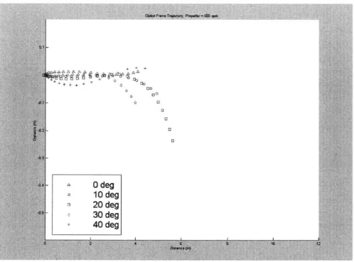
At 500 RPM, the data appeared to show that a twenty-degree rudder was more effective at generating a rapid turn than the other angles. The zero and forty-degree rudder angles appeared to have little to no effect in turning the boat to starboard, with the ten and thirty degree angles showing intermediate results.

Figure 29 Trajectory Followed by Ship Model at 600 RPM with Varying Rudder Angle At 600 RPM, similar trends also appear with zero and forty-degree rudder angles having similar effects in guiding the boat, while intermediate rudder angles showed more signs of effectiveness within the span of the testing period.

(47)

Figure 30 Trajectory Followed by Ship Model at 700 RPM with Varying Rudder Angle

Figure 31 Trajectory Followed by Ship Model at 800 RPM with Varying Rudder Angle At 700 and 800 RPM, the ten degree rudder angle appeared to have significantly less turning effect on the ship than the other angles, and the forty degree rudder angle appeared to have a similar turning effect as other rudder angles, but with a cost in the total track length. For large angles of attack, the rudder may have been generating a significant portion of its turning moment from pure drag rather than lift, thus creating a

(48)

shorter track length while still managing to turn effectively. At lower speeds, the loss in lift may not have been sufficiently compensated by the increase in drag in order to create a turn to starboard.

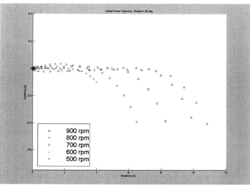
Figure 32 Trajectory Followed by Ship Model at 900 RPM with Varying Rudder Angle

At 900 RPM, the data seemed to indicate a high turning effectiveness from ten, thirty and forty degree rudder angles. The actual track length and the deviation from the straight path of the twenty degree rudder is difficult to discern given its initial turn to port before returning to a starboard turn.

(49)

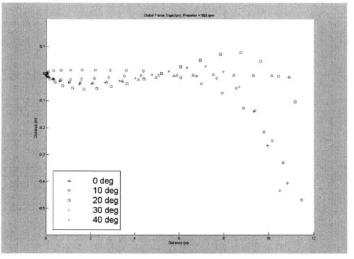
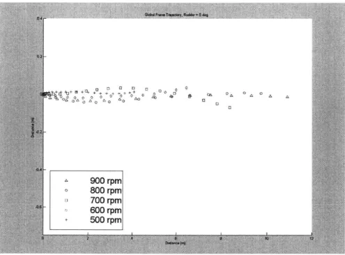
Figure 33 Trajectory Followed by Ship Model with 0 degree Rudder Angle and Varying RPM The plot above and the series that it begins are also scatter plots of the trajectory followed by the ship for different speeds and the same rudder angle. Motion along in the y-direction remained fairly limited, which was the expected result. Relative distances traveled appeared to be reasonably proportionate to the relative speed at which the propeller turned.

In the following plots, the relative effectiveness of intermediate rudder angles at producing a turn may be seen for a range of speeds. Ten and forty degree rudder angles appear to be too small and too great respectively to generate optimum performance at the speeds reached using higher RPM within the tank. The forty-degree rudder does manage to provide a decent turn, but only for the 900-RPM trajectory.

(50)

Figure 34 Trajectory Followed by Ship Model with 10 degree Rudder Angle and Varying RPM

(51)

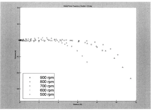
Figure 36 Trajectory Followed by Ship Model with 30 degree Rudder Angle and Varying RPM

(52)

Figure 38 Changes in Heading Using Various Rudder Angles at 500 RPM

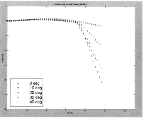
The heading angle plot for different speeds adds to the picture of what the ship is doing as it begins a turn, begins to decelerate, and drifts towards the wall of the towing tank. In the plots for various speeds, the ultimate heading angle reached for different speeds increases with increasing speeds, as may be expected since greater velocities mean greater drag effects which contribute to the turning rate.

The effectiveness of different rudder angles may again be compared, and for heading, the results are more uniform. Turning angle reached increases with increasing rudder angle until the forty degree rudder was used, which provided mediocre response until higher speeds were reached.

(53)

(54)

(55)

Figure 43 Changes in Heading for Several RPM Using 0 degree Rudder

Again, the greater effectiveness of higher speeds in making turns is well evident in the plots of heading angle as a function of speed for each rudder angle

(56)

Figure 45 Changes in Heading for Several RPM Using 20 degree Rudder

(57)

Figure 47 Changes in Heading for Several RPM Using 40 degrees Rudder

For the effects on forward velocity from changes in rudder angle at various speeds, see Appendix A.