Design and Parametric Simulation of Radially
Oriented Electromagnetic Actuators "^S
by
Will Bosworth
Submitted to the Department of Mechanical Engineering
in partial fulfillment of the requirements for the degree of
Masters of Science in Mechanical Engineering
at the
MASSACHUSETTS INSTITUTE OF TECHNOLOGY
June 2011
@
Massachusetts Institute of Technology 2011. All rights reserved.
A uthor
...
...
...
Department of Mechanical Engineering
/I 15>2 / /7
May 20, 2011
Certified by...
Jeffrey H. Lang
Professor of Electrical Engineering and Computer Science
Thesis Supervisor
Certified by...
...
...
exander H. Slocum
Professor of Mechanical Engineering
Thesis Supervisor
Accepted by ...
David E. Hardt
Professor of Mechanical Engineering
Graduate Officer
Design and Parametric Simulation of Radially Oriented
Electromagnetic Actuators
by
Will Bosworth
Submitted to the Department of Mechanical Engineering on May 20, 2011, in partial fulfillment of the
requirements for the degree of
Masters of Science in Mechanical Engineering
Abstract
This thesis presents the design and simulation of an electromagnetic actuator system capable of delivering large pulses of radial force onto a cylindrical surface. Due to its robust design, simple control scheme, and large output force capability, the actuator design is developed to be considered for wellbore manipulation and other downhole oil exploration and production activities.
The complete simulation - including capacitor bank power supply, solid state switch-ing circuit, transducer, and target formation - is a thirteen value lumped parameter model. The simulation was used heavily in the design and refining of two experimental prototype systems. These prototypes showed excellent model-experiment matching. The experimental prototypes are 2.5" radius, 12" length cylindrical transducers that exert nearly 10 psi onto a simulated rock formation with 2 MN/m radial stiffness, increasing the formation radius 3.5 mm during 5 ms pulse events.
It is with this experimentally validated simulation that we project forward a man-ufacturable system capable of exerting pulses of hundreds of psi in magnitude over durations of 1 - 10 ms onto wellbore sized cylindrical surfaces.
Thesis Supervisor: Jeffrey H. Lang
Title: Professor of Electrical Engineering and Computer Science Thesis Supervisor: Alexander H. Slocum
Acknowledgments
This work was funded by Schlumberger and performed at MIT, directly enabled through the guidance of Professor Jeff Lang and Dr. Julio Guerrerro, and furthered along with efforts from Professor Alex Slocum, Dr. Jahir Pabon, and Alec Resnick.
Contents
1 Introduction
1.1 The Pulsed Electromagnetic Radial Actuator System . . . .
1.2 Motivation and Prior Art... . . . .
1.3 T hesis Structure . . . . 2 Radially Oriented Electromagnetic Transducer
2.1 Lorentz Force Law on a Wire Review ... 2.2 Conductor Layout for Radial Actuation . . . . .
2.3 Magnetic Field of the Axial-Current Layout . . 2.4 Self Induced Electromagnetic Force . . . .
2.5 Inductance of the Axial Current Layout . . . . .
2.6 Transducer Resistance . . . .
3 Power Supply, Electrical Energy Model, Mechanical Energy Model 3.1 Capacitor Bank and Power Circuit . . . . 3.2 Discharging Capacitor Circuit: Modeling Current Flow Through the
T ransducer . . . .
3.3 Mechanical Force/Displacement State Equations . . . . 3.4 Estimating Formation Properties Downhole . . . .
4 Assembling the Full Parametric Simulation
4.1 System Param eters . . . . 4.2 State Equations . . . . 19 . . . . 20 . . . . 21 . . . . 23 . . . . 25 . . . . 25 . . . . 27 29 29 30 32 33 35 35 36
4.3 Energy Balance in the Simulation Output . . . . 37
4.4 Viewing Output Data. . . . . 38
5 The Radial Actuator Prototype and Characterization 41 5.1 Specifying Parameters for the Initial Prototype . . . . 42
5.1.1 Parameter Search Using the Simulation . . . . 44
5.2 Prototype Machine Design . . . . 48
5.2.1 Transducer and Formation Design . . . . 48
5.2.2 Capacitor Bank and Circuit Components . . . . 53
5.3 Alpha Prototype Characterization . . . . 54
5.3.1 Static M easurements . . . . 55
5.3.2 Dynamic Measurements: Setup . . . . 57
5.3.3 Dynamic Measurements: Alpha Prototype Experimental Results 59 6 The Second Radial Actuator Prototype 61 6.1 Litz Wire Transducer Design . . . . 61
6.2 Characterizing the Beta Prototype . . . . 64
6.3 Comparing Performance of Alpha and Beta Prototypes . . . . 67
7 Simulation Results for Wellbore Applications 71 7.1 An Actuator Design for Increasing Wellbore Radius . . . . 72
7.2 An Actuator Design for Creating Impulse Waves for Seismic Analysis 75 7.3 Selecting the Simulation Parameters Used in This Chapter . . . . 75
8 Conclusion 81
List of Figures
1-1 PEM schematic... . . . . . . . . .
2-1 Current carrying wire in a magnetic field . . . . 2-2 Radial electromagnetic force layouts. On the left, current moves
axi-ally and magnetic field circulates. On the right, magnetic field moves axially and current circulates. . . . ...
2-3 Axial and Azimuthal current layouts for radial force. The axial current
2-4 2-5 2-6 3-1 3-2 3-3 3-4
layout is the focus of this thesis . . . . Axial current layout for Ampere analysis . . . . Faraday surface . . . . Cylinders with radius, thickness, and number of turns Energy flow overview . . . . Power circuit . . . . RLC circuit and KVL polarity definitions.. . . ..
Mass spring damper model . . . . 4-1 Simulated energy flow . . . .
4-2 Simulation output: (a) outer radius extension, (b) current tance, and (d) voltage in simulation . . . .
. . . . 23 . . . . 24 . . . . 26 . . . . 28 induc-. . . . . . 40
5-2 Parameter Sweeping C and K... . . . . 5-3 Radial Displacement with Varying K . . . .
5-4
5-5 5-6 5-7 5-8
Cross section of transducer and radial stiffness . . . . Orhtographic view of experimental device... . . . .. FEA result for 800N loads on each spring . . . .
Plastic connection detail feature view . . . . Completed Alpha Prototype Transducer, Formation, and Capacitor Bank
5-9 Complete Alpha Prototype Experimental Setup 5-10 5-11 5-12 5-13 6-1 6-2 6-3 6-4 6-5
Measuring Capacitor R and C . . . . Non-contact inductive sensor on prototype . . . . Schematic of measuring voltage across a real capacitor
Alpha Prototype Experimental and Simulated Actuator Event Model of Beta Prototype.. . . . . . ..
Beta Transducer Assembly Line . . . .
Beta Transducer Assembly in Progress . . . .
Assembled Beta Transducer . . . . Complete Beta Prototype Actuator . . . .
50 51 52 52 53 54 56 58 59 60 . . . . . . . . . . . . . 63 . . . . . 64 . . . . 6 5 . . . . 66 . . . . 6 7
6-6 Experimental and Simulated Actuator Event - Beta-Prototype . . . . 6-7 Simulated Energy Transfer of Experimentally Validated Prototypes
7-1 Outer Radius Displacement . . . .
7-2 C urrent . . . . 7-3 Electromagnetic Force on Conductors . . . . 7-4 Energy Balance . . . .
78
7-6 Simulation of current using best parameters from sweeps of Figure 7-5 79 79 79
List of Tables
4.1 Simulation input parameters . . . . 36
4.2 Simulation system states . . . . 36
4.3 System parameters used in Section 4.4 output viewgraphs . . . . 38
5.1 Simulation input parameters . . . . 42
5.2 Refining simulation input parameters... . . . . . . . 45
5.3 Simulation input parameters for parameter sweep . . . . 45
5.4 Constrained input parameters for initial prototype design . . . . 48
5.5 Statically measured values of alpha prototype.. . . . . . . . 57
5.6 Purchased parts.... . . . . . . . 57
6.1 Statically measured values of beta prototype . . . . 64
Chapter 1
Introduction
This thesis concerns the design and simulation of an electromagnetic actuator that creates large magnitude short duration force pulses oriented radially outward. The system was first proposed while brainstorming solutions to a wellbore manipulation challenge. the actuator had inherent features that made it intriguing to apply to the oil service industry: it could have a compact robust package suitable for harsh down hole environments, a simple yet repeatable and precise control scheme, and could achieve impressive power density. It seemed that this electromagnetic actuator could compete with explosive charges and hydraulic actuators in some downhole applica-tions, so we set out to provide tools and analysis to enable further development. We created a nonlinear thirteen parameter electromechanical simulation of the sys-tem. The simulation was used to design prototypes which were used to experimentally validate the simulation. The prototypes also enabled us to develop and refine tech-niques for designing and building such systems.
We used the experimentally validated simulation, along with estimates of downhole formation properties and availiable electrical and mechanical components, to predict the capability of such systems in the field. We show that manufacturable versions of this system could apply hundreds of psi onto a cylindrical wellbore surface in 1 - 10
nearly 1 m/s.
The remainder of this chapter presents a brief technical overview of the actuator system, describes prior art that motivated our design, and presents the layout of the complete thesis document.
1.1
The Pulsed Electromagnetic Radial Actuator
System
The actuator systems described herein have a capacitor bank that delivers electrical energy to an electromagnetic transducer where electrical energy is converted into mechanical energy. The capacitor bank and switching circuit are called the power supply, the device where electrical and mechanical energy conversion takes place is called the transducer, and the mechanical system that is acted upon by the mechanical force is called the formation. In this document, the formations of interest are the rock formations in which a wellbore hole exists.
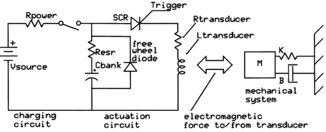
A lumped parameter schematic of the electrical and mechanical system is shown
in Figure 1-1. A capacitor bank discharges current into the transducer, which is represented electrically as an inductor and resistor, and mechanically as a force source. Electrical energy is converted into mechanical energy inside the transducer and force is delivered to the formation. In this thesis the formation is modeled as a linear mass-spring-damper system, though other physical models could be applied. From this perspective, the system model is an LRC circuit connected to a mass-spring-damper mechanical model through the electromagnetic transducer.
Electromagnetic actuators often use permanent magnets and/or soft magnetic materi-als in the generation of force which can lead to saturation issues at high current/force. The actuator design presented herein does not use magnetic materials; instead, cur-rents traveling through conductors induce magnetic fields that interact to generate forces. The advantage of an all-copper actuator is that much greater force can be
charging actuation circuit circuit
K
MB mechanical system electromagneticforce to/from transducer Figure 1-1: PEM schematic
generated without saturation or damage to permanent magnets. Additionally, an all-copper actuator can handle more extreme temperature and chemical environments than an actuator that includes permanent magnets. Though, over operating con-ditions in which permanent magnets can perform, the permanent magnet actuators will typically require less current to achieve the same force output and thus generally operate more efficiently.
1.2
Motivation and Prior Art
The actuator system developed in this thesis is a direct extension of a patented work by Wilson and the Carrier Corporation [7] which describes an electromagnetic actuator to plastically deform metal tubes and plates. This thesis builds on the radial actuator concept, presenting a parameterized actuator system design and simulation tool to enable design engineers to assess and optimize system performance for their own applications.
In non-radial coordinates, the most common pulsed electromagnetic induction actu-ator is the rail gun. A rail gun uses induced magnetic fields to accelerate projectiles in a straight line. The United States Navy has been developing rail guns for long range missile launch and for ship based aircraft launch applications [8], [9], [1]. These
launchers are being considered because they can compete with explosive based, pneu-matic, and hydraulic systems in pure kinetic-energy creation (exit velocity of projec-tile), but also because the electromagnetic system can be more robust, repeatable, and offers the ability to modify/control launch parameters in real time (so, the same launcher can be designed to optimally launch different types of projectiles).
Pulsed power electromagnetic actuators have also been used as the signal source for non-contact vibration based sensors. A capacitor bank driven transducer system was developed and used by Edgerton in the 1960's to map the bottom surfaces of lakes and rivers that were too deep, too murky, and too varying to use vision or contact based techniques [4], [5].
High speed/force electromagnetic actuators were presented as early as 1919 [2] but generally have not made it into practical implementation until recently. A number of technologies and realizations have come together recently that make electricity based actuation a compelling option for high force applications. Solid state switches, a technology that enabled the consumer electronics industry we know today, have become capable of switching very large amounts of current very quickly, efficiently, and predictably. Though, switches are still often the limiting factor in increasing high power electromagnetic system performance [3]. Battery and capacitor perfor-mance continues to improve, increasing the achievable power and energy densities that can be delivered electrically. Also, pervasive computation and numerical simula-tion techniques make system design and optimizasimula-tion a faster and intellectually more manageable process.
1.3
Thesis Structure
This document takes the following structure:
* Chapter 1 presents the concept of using pulsed electromagnetic induction actu-ators to create high peak short duration mechanical force pulses and describes
the general features of such a system. Potential uses of a radially acting PEMI system for oil exploration and completion activities is discussed and the need for a parametric simulation to aid in assessing viability is presented.
" Chapter 2 describes the conductor layout of an induced magnetic field trans-ducer that results in radial force. The relationship between electrical current, induced magnetic field, and mechanical force is derived in terms of the relevant parameters (conductor material properties and geometry) that will be used in the simulation.
" Chapter 3 presents the design and modeling of the power supply/circuit and of the mechanical formation. The relationship between electrical and mechanical parameters to the time varying performance of the simulation are presented. " Chapter 4 assembles the three modules (the transducer, power supply, and
me-chanical formation) into a single four-state time varying simulation and sum-marizes all of the relevant parameters that affect system performance.
" Chapter 5 describes the design and characterization of the first experimental prototype. Design decisions and the use of the simulation to aid in parameter selection are documented. The manufactured actuator system and the sensors used to measure performance are presented. Finally, successful matching of model and measured system performance is shown, and factors that limit system performance are discussed.
" Chapter 6 describes an improved transducer design and additional experimental validation. Here, a second method for conductor layout was developed; the expected improvements of this modification were validated by the simulation tool before manufacture, and confirmed experimentally. The transducer design presented here is used as the basis for simulation results of the next chapter. " Chapter 7 presents simulation results that demonstrate the viability of this
type of actuator to rapidly mechanically deform wellbores mechanically at a high axial rate down the wellbore.
* Chapter 8 summarizes the development and performance of the parametric simulation tool and describes some limitations and potential extensions of the project.
Chapter 2
Radially Oriented Electromagnetic
Transducer
This chapter presents the design of a radially oriented electromagnetic transducer. In overview, a transducer converts electrical and mechanical energies by the following processes:
e When current flows through a wire, a magnetic field is created. This
phe-nomenon is described by Ampere's Law and Gauss's Law.
e When the magnetic field from one wire interacts with current of another wire,
a force is created. The direction and magnitude of the force created by the interaction of current in a magnetic field is described by the Lorentz Force Law. * How a conductor or set of conductors creates a terminal voltage from its ter-minal voltage and motion affects how the device interacts with other electrical components. This relationship is described by the device's inductance, defined in Faraday's Law.
e The size and length of the wires in a device affect the resistance of that device,
2.1
Lorentz Force Law on a Wire Review
The Lorentz force law relates how electric and magnetic fields interact with point charges to create force. The force f on a single charge in free space is described by:
f
= q[E + (u x po H)]. (2.1)Here, f is the force, E the electric field, H the magnetic flux, yo the permitivity of free space, q the electric charge of the particle, and u the velocity of the particle. From this point forward, the following relationship will be used for magnetic flux
density B, magnetic field H, and pto:
B = po H. (2.2)
A current carrying wire contains many individual moving point charges. When a
current carrying wire is in the presence of electric or magnetic fields, the total force on the wire will be a summation of the individual forces on each point charge. This total wire force is derived as follows, citing the geometry described in Figure 2-1. Given a current flux J as
J = q Ndu, (2.3)
and force distribution F defined as
F
f
Nd, (2.4)where Nd is a volume distribution of charges charge]) moving with velocity u. Then, Equation 2.1 can be modified to become
f
Nd= qu Nd x B(2.5)
The electric force has been discarded under the assumption that the wire in Figure 2-1 is charge neutral.
Given the definition of F, the geometric relationship to the current carrying wire as shown in Figure 2-1 is
(2.6)
f
=FAW.Substituting Equation 2.5 into Equation 2.6 leads to
f
= (J x B)AW. (2.7)Since current i and current flux J are related as
i=JA.
Then, the macroscopic force on a wire within a magnetic field can be written as
fwire = i W x B.
(2.8)
(2.9)
2.2
Conductor Layout for Radial Actuation
A uniform radially outward force can be achieved by either having a magnetic field
circulate rotationally while a current moves axially on the cylinder or having a mag-netic field point axially while a current circulates around the cylinder. These two orientations are shown in Figure 2-2.
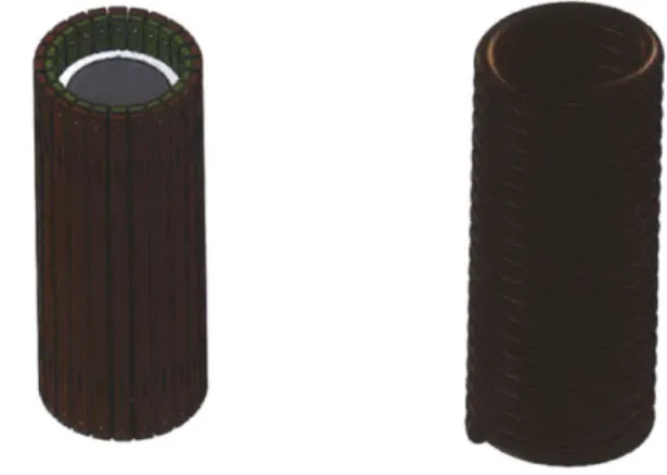
Using copper wires, the axial current design could be achieved using a layout shown on the left of Figure 2-3. In this figure current could travel 'up' the inner green wires and 'down' the outer brown wires; the connections between the inner and outer are not shown in the figure. Alternatively, the azimuthal-current layout would look like
magnetic field B cross section A current flux J, current i = J A lengthW
A
Figure 2-1: Current carrying wire in a magnetic fieldFigure 2-2: Radial electromagnetic force layouts. On the left, current moves axially and magnetic field circulates. On the right, magnetic field moves axially and current circulates.
Figure 2-3: Axial and Azimuthal current layouts for radial force. The axial current layout is the focus of this thesis
that shown on the right in Figure 2-3.
The axial current layout is more practical for creating a radial actuator that translates radially; though one must design properly compliant connections between the inner and outer sets of wires. The remainder of this thesis focuses solely on the axial current layout.
2.3
Magnetic Field of the Axial-Current Layout
When current travels through the transducer a magnetic field is created that interacts with the current to create force. The magnetic field is quantified by applying Ampere's Law:
B -dl iA enclosed. (2.10)
A top view schematic of the axial current layout is shown in Figure 2-4. The inner and
outer wires are in series; if current is traveling up (out of the page) the inner conductor loop, it is traveling down (into the page) the outer loop. The surface enclosing region 1 has zero current and thus no magnetic field. In region 2 the magnetic field includes current of the inner conducting loop, and the magnetic field is evaluated by summing
outer conductor cylinder (current traveling down)
inner conductor cylinder (current traveling up) region
1 2 3
Figure 2-4: Axial current layout for Ampere analysis
the enclosed current over the circular path:
2 7r 0 rO enlsd H = ~ 27 r B = 901. 27r r (2.11) (2.12) (2.13)
Region 3 of Figure 2-4 encloses a total of zero current, since the axial currents of the inner and outer wires cancel each other out. This is results in zero magnetic field outside of the outer set of wires.
If the axial layout had many turns of wire in series, the resulting magnetic field would
include N turns (which is not the same as charge density Nd):
B 0 N I
B -(2.14
2.4
Self Induced Electromagnetic Force
The Lorentz force law can now be applied to the axial-conductor layout. Neglecting fringe effects, the magnetic field is constant along the length of the cylinder and pointed radially outward at all points on the the outer set of wires (and radially inward on the inner wires).
Fem,outer = -N iWB = poWN 2 (2.15)
2 2 7r router
where Wz is the axial length of the cylindrical actuator.
The
j
term in above equation accounts for the tapering of the magnetic flux from the inner-most point of the outer conductor to the outer most point - at the inner surface of the outer conductor loop the enclosed current is encloccd. But, at the very outer edge of the outer conductor, the enclosed current is zero, since the total current is the current traveling up the inner conductor loop and back down the outer conductor loop. Thus, over the thickness of the outer conductor loop, the average enclosed current is one half the total enclosed current.The force is evenly distributed radially outward on the surface of the cylinder, thus the pressure exerted on the cylinder is
Fem,outer __ o N2 2
Pwellbore 7 ro W z -2 A ir2 r2.1'
2.5
Inductance of the Axial Current Layout
The inductance of the actuator is derived by applying Faraday's Law,
ri ro axis of rotation
Figure 2-5: Faraday surface
where
<D J B ds.
<D is the magnetic flux, and A is the flux linkage.
(2.18)
Figure 2-5 describes the surface used to analyze Faraday's law. Here, a cross section view of the cylindrical actuator is shown lying with the z-axis horizontal. The Faraday surface spans the length of the cylinder from the inner to outer surface (the red dashed line).
A is further computed from Equations 2.17 and 2.18, substituting B from
Equa-tion 2.13, as
A = r
o 27r
r Lt. (2.19)
Thus, inductance, as a time varying function of the outer radius r,(t) is
Ipo Wz N2
L(t) = 2
2.6
Transducer Resistance
The resistance of the transducer is determined by conductor geometry - length and cross section - and conductor resistivity:
Rtransducer = Plc (2.21)
where Rtransducer is the resistance, p the resistivity, lc the conductor length, and Ac the conductor cross sectional area.
Total conductor length is a function of axial length Wz and turns N, as well as the length of the end-turn wires that connect the inner and outer axial wires together. One end turn connector is length tend. Therefore,
lc = 2 NWz + 2Nend. (2.22)
The length of the end turn plays a limiting role in the maximum radial travel of the transducer; increasing the maximum travel distance will increase resistance of the transducer, which can limit current and maximum force.
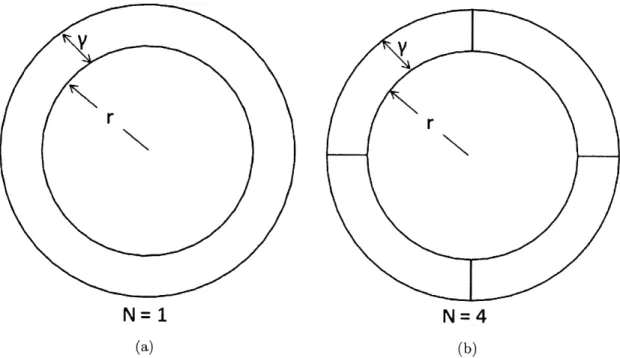
The calculation of any real Ac depends on attainable conductor geometry but the following example shows how Ac is a function of turns N, conductor thickness -y, and transducer radius r. Figure 2-6 shows two cylinders with cross section, radius, and number of turns. Each cylinder could represent either the inner or outer conductor set of the transducer.
Ac = 7 ((r±+ r2) (2.23)
N
The N = 4 case would have a quarter the cross sectional area and four times the conductor length, so the ratio of the total resistance of the N = 4 cylindrical conductor to the N = 1 conductor is 16 - or more importantly, N2
N=1 N=4
(a) (b)
Chapter 3
Power Supply, Electrical Energy
Model, Mechanical Energy Model
This chapter specifies and simulates the electrical power system that delivers electrical energy to the transducer, and the mechanical system (the formation) upon which the transducer acts upon. A schematic of the energy domains modeled here are described described in Figure 3-1.
3.1
Capacitor Bank and Power Circuit
As seen in Equation 2.15, force out of the transducer goes up with the square of current. If the goal of the system is to create large forces, the goal of the electrical system design is to create large currents. Discharging a capacitor into a low resistance and low inductance circuit is a common method for creating a short burst of large
electrical mechanica
energy energy
Rtransducer
Vsource Cbank r Ltransducer
charging actuation
circuit circuit
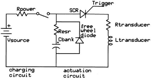
Figure 3-2: Power circuit current.
The electrical circuit is shown in Figure 3-2. A charged capacitor bank is triggered by a silicon controlled rectifier (SCR). An SCR is a solid state switch that can stand-off large voltages until triggered by a low energy control signal. The SCR can carry thousands of amps of current and typically has a fraction of a milliohm of resistance, making it a nearly ideal, lossless switch. The capacitors are charged by closing the switch to a DC voltage source; given proper duty cycle, the capacitors will reach the voltage of the charging supply.
3.2
Discharging Capacitor Circuit: Modeling
Cur-rent Flow Through the Transducer
The actuation circuit can be simplified to the RLC circuit shown in Figure 3-3. The capacitor contributes the dominant capacitance term and the transducer the dominant inductance term (every component has a little bit of inductance, capacitance, and resistance). The transducer wires, capacitor bank, connecting wires, and SCR all contribute to the circuit's parasitic resistance.
i
Rparasitic Vr-TCbank
+
Ltransducer o
actuation circuit
Figure 3-3: RLC circuit and KVL polarity definitions
Kirchoff's voltage and current laws and introducing the flux linkage A, resulting in Equations 3.1: through 3.6. KVL: Vc - V, - VL=0 (3.1) KCL: -c =z=L i (3.2) flux linkage: A- L i VL dt (3-3) dA AR d= VL Vc- V c-iR =Vc (3.4) dt L dVe - = - = -i --A (3.5) dt C LC d A - I A (3.6) dt v -1 0 V
Flux linkage A is chosen as a state rather than current i since inductance L is not constant throughout the time varying simulation. The state equations in Equation 3.6 are used in the time-varying simulation of voltage and current during the capacitor discharge event. These state equations will be combined with the mechanical system state equations to form the full electro-mechanical simulation in Chapter 4.
Two components in the actuation circuit schematic of Figure 3-2 are not included in the simplified schematic (and related model) of Figure 3-3: the SCR and the freewheeling diode. Once triggered, the SCR remains closed as long as current is flowing from anode to cathode. The switch latches opens when current approaches zero. Pure RLC circuits may exhibit large negative voltage and current swings; an RLC circuit controlled by an SCR will not experience the same transient response as a pure RLC circuit beyond the first zero crossing of current. Though, nearly all useful energy transfer occurs before current swings to negative in the RLC circuit, so the straightforward RLC model is valid for the important parts of the actuation event.
A flyback diode is necasarry to protect the capacitor bank from large reverse voltages
which is necessary for the integrity of electrolytic capacitors used in this power supply.
A simulation using the state equations in Equation 3.6 will only resemble reality
through the initial voltage drop to zero.
3.3
Mechanical Force/Displacement State
Equa-tions
The actuator system is designed to do work on a formation by applying radial force. Simulating the mechanical system is an important part of understanding system per-formance. Figure 3-4 shows the simplified formation model used in the simulation. The spring constant and damping of the stiff outer formation are treated as linear, therefore the state equations for formation displacement can be described through simple application of Newton's first law, with the full state described in Equation 3.8. Note that Equations 3.7 and 3.8 are written with variable r to denote radial dis-placement.
mechanical
system
force to/from transducer
Figure 3-4: Mass spring damper model
d + Fradial (3.8)
A similar force will occur radially inwards on the inner wires of the transducer. The
transducer should be designed such that the inner wires are mounted in a very stiff configuration and thus displace negligibly.
3.4
Estimating Formation Properties Downhole
The stiffness of wellbores downhole is estimated using Young's modulus values in
[10], combined with a thick walled cylinder approximation described in Equation 3.9
from [11]. In Equation 3.9, a is the wellbore diameter, and b is much greater than a.
p is pressure applied to the wellbore, E the formation Young's modulus, and v the
Poisson's ratio. The stiffness of the formation is given by Equation 3.16 and derived as follows.
A a p) (a2
+
b2E (b2- 2 V) (3.9)
a2
+
b2b2 -a 2 when b
>
a (3.10)define wellbore diameter: d_ = a (3.11)
Adw = d, pv (3.12) E p A = F = K Adw (3.13) A =7r dw Wz (3.14) K = (3.15) Adw gW, EN Kradial - = (3.16) V m
The Young's modulus values of interest range from 0.01 to greater than 10 GPa, values associated with soft/unconsolidated sandstone to highly consolidated sandstone. This results in an estimated wellbore stiffness from about 107 to 1010 N/r.
Chapter 4
Assembling the Full Parametric
Simulation
This section documents the full parametric simulation of the radial actuator system. This includes the system parameters (inputs), state equations, and useful simulation outputs. A complete implementation of this simulation in MATLAB is provided in Appendix A.
The conversion of electrical energy from the capacitor bank to mechanical energy in the formation via the electromagnetic transducer is modeled as a four state set of differential equations. All of the variables and equations in this section were derived in the previous transducer, power supply, and formation modeling sections (Chapters 2 and 3).
4.1
System Parameters
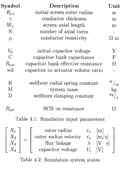
Table 4.1 shows the input parameters that define the simulation. This list includes relevant parameters of the transducer, the power supply, and the formation.
Description
initial screen outer radius conductor thickness
screen axial length number of axial turns
conductor resistivity initial capacitor voltage capacitor bank capacitance
Resr capacitor bank effective resistance
vol capacitor to actuator volume ratio K wellbore radial spring constant
M system mass
D wellbore damping constant
Rscr SCR on resistance
Table 4.1: Simulation input parameters
Symbol N/rn kg k9/s Q X1 outer radius
X2 _ outer radius velocity
X3 flux linkage X4 capacitor voltage
ro
[ml
ro [m/s] A [V s] V [V]Table 4.2: Simulation system states inner and outer radius are close to each other, then
Rrnne= Ro,j -T. (4.1)
The system states that will be used to solve the ODE's are shown in Table 4.2. The first two states are displacement and velocity of the mass spring damper system, and the second two states are related to voltage and current of the electrical system.
4.2
State Equations
In numerical simulation, a state update is performed every time step dt. The state update equations are shown in Equation 4.2, incorporating the global constants from
Unit m m m Qm V F Q Wz N p
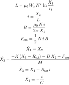
Table 4.1. L - ptoW_ N2 In
,i-x
3 .X3 L B - poN i 2 7r X1 1 FerM - NiB 2 (4.2) -K (X1 - Ro,2) - DX 2 + Fern 3 = X4- Rtot i X4 =-Due to the electrical implementation (the SCR and the freewheeling diode), the set of update equations in Equation 4.2 is valid until V = 0 or iL < 0.
4.3
Energy Balance in the Simulation Output
Energy must be conserved in each time step of a valid simulation result less rounding errors, this relationship is given by Equation 4.3.
Param Static Measured Cbank 0.24 ESRcapBank 2.8 Ro'i 55 Ri 45 N 24 Rtransducer 1.8 Ltransducer,i 7 K 2.32
Table 4.3: System parameters used in Section
Unit F mQ mm mm mQ MN 4.4 output viewgraphs The energy domains relevant to this system are described in Equation 4.4.
Ecapacitor = 1 C V2 1 -2 1 Espring =K Ar2 21 Ekinetic = M r 2 = Eresistance =
Ji
2R dt (4.4) EdamperJ
TD
dt
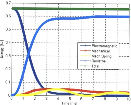
Accounting for energy flow across the various electrical and mechanical domains is useful as a sanity check - if Equation 4.3 is not satisfied something is very wrong. And, since the point of this actuator system is to transfer electrical energy into me-chanical energy, viewing the energy flows in a simulation result is useful for comparing system designs across different size/energy scales.
4.4
Viewing Output Data
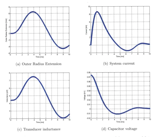
The graphs in Figure 4-2 show some of the key output data of the simulation. The simulated flow of energy, as described in Equation 4.4, is shown in Figure 4-1. This figure is from the same simulation result as Figure 4-2.
--- ---- Electromagnetic - - -- - -- - --- - - --- -- - - - - ---- Mechanical ---- --- --- --- - -- --- -- --- M ech Spring - - ----*- Resistive ilip -±- Total U 1 2 3 4 5 6 7 8 9 10 Time [ms]
Figure 4- 1: Simulated energy flow 0.7 0.6 0.5 0.4 0.3 0.2 0.1
0 2 - --- -- -. --- --- --- - - - - .. -4 .. .. -2- - 2 3- -- 6 7 8 --- --- | |--- U0 1 2 3 4 5 6 7 8 9 10 Time [ims]
(a) Outer Radius Extension
e 7 -- -- --- -- ---- - ---... --- --- - ---I -6 --- .... .. --- - - ---- +- - - -- -- -- -- - -- -5 ---... .. .-... -- --- --- --- --- -- - --. -.. . - ---. 4 - ---- --- - ---- - - - -- - 6-0 1 2 3 4 5 6 7 8 9 10 Time [ms] (c) Transducer inductance 6 2 1 1 2 3 4 5 6 7 8 9 10 Time [ms] (b) System current 0. 0. 0. 0. 0 -0 0, -0 07 07 -- ---- -- --- -- - --- - - - -- --- - -- ---06 --- -- - - - - - --- --- --- -- - - -- - - - ---- -- -04 --- -... . .. I.. . .I- - - - -- --- - - --- -- - -03 -- -- -- -.. . . .. . .. -- - - -- - -- -- - --- - - - - -02 - +--- -- - +--- +---+--- - --- -- -01 -- --- - --- - ---- --- - ---0 ---- - --. -- --. --- -- --- - -- .. -. 01 --- + - -01 m1 2 e 5 [1 Time [ms] (d) Capacitor voltage
Figure 4-2: Simulation output: (a) outer radius extension, (b) current , (c) induc-tance, and (d) voltage in simulation
40
-- - -- -- --- --- --- ---- --
-. . .1 I - |
31I
Chapter 5
The Radial Actuator Prototype
and Characterization
This chapter begins the second part of the thesis: creating and evaluating real ac-tuation system designs using the design framework and parametric simulation tool developed in Chapters 2 through 4. The necessity of building real systems is two-fold. First, a real system must be made and characterized in order to validate the simulation; that is, the simulation must be proven experimentally. Second, to move beyond simulation and into functional device design, the simulation parameters must be connected to a real system layout made of real materials and components.
Two prototype actuator systems were built and experimentally characterized. The complete design of these actuators and the experimental setup and methods used to characterize are described here. The story of this design, manufacture, and ex-perimental characterization will be told chronologically. The author feels that many insights of this work - both as a designer of things and as a designer of pulsed
induction radial actuators - will be gleaned most from the design story. See Sub-sections 5.3 and 6.2 to jump straight to the prototype dimensions/parameters and experimental results.
Symbol RO' -y Wz N p V C Resr vol K M D Rsecr Description
initial screen outer radius conductor thickness screen axial length number of axial turns conductor resistivity initial capacitor voltage
capacitor bank capaci-tance
capacitor bank effective resistance
capacitor to actuator vol-ume ratio
wellbore radial spring con-stant
system mass
wellbore damping con-stant
SCR on resistance
Table 5.1: Simulation input parameters
5.1
Specifying Parameters for the Initial
Proto-type
As shown in Table 4.1 on page 36 the system model is defined by thirteen lumped
parameters related to the actuator. Five parameters completely define the transducer design and performance, four define the capacitor bank performance, three define the formation, and one the SCR electrical switch. Thirteen parameters is a lot of values to choose at once; a starting point for guiding parameter specification is described in Table 5.1 and discussed here.
A wellbore is commonly 5 to 36 inches in diameter, though the diameter of tools that
will be inserted into the well are typically about half the wellbore diameter, putting a scaled prototype tool around 2.5 to 18 inches in diameter.
To avoid fringe effects in applying Ampere's and Faraday's Laws, the axial length should be larger than the radius (W, > 3 R0,). Avoiding fringe effects is useful for
model accuracy, but also because fringe magnetic fields do not contribute to useful
Requirement
wellbore sized
small enough to allow thin conductor approximation long enough to make edge effects negligible
small enough to be practical to assemble by hand the smaller the better
high enough to be interesting, low enough to simplify design and safety requirements
same as above
the smaller the better
1:1 desirable, do not want too large
stiff enough to be interesting, small enough that dis-placement can be measured without huge forces or obscure sensors
something practical for experiment: low
force generation at the transducer. Thus, if the axial length is set to 12 inches (large enough to be interesting, but can still easily fit on a lab bench), then the radius may be set to around 4 inches.
A rough sizing of the capacitor bank can be made by relating the expected volume
of the transducer and the energy density of the capacitors in the capacitor bank. This tool prototype specifies that the volume of the capacitor bank be approximately the same as the volume of the transducer itself. The energy density of capacitors is estimated as 0.18 MJ/m 3 using a data sheet for high temperature capacitors from Vishay [12]. Thus, the capacitance and maximum operating voltage of the capacitor bank can be sized as a function of volume as in Equation 5.1. Specifying capacitor performance with high temperature capacitors is important for this design because the tool should be capable of operating in extreme environments downhole (even though the actual experimental device does not use specialty capacitors).
V0ltransducer 7 2?r I CV2 [j] vol cap -~V J Vo~cap 2Edensity volcap voltransducer (5.1) 2 Edensity 7r r2 Wz 2(0.176e6) r 0.0552 (0.3) 0 C ~ =-0.18 752
Operating at high voltages increases system design complexity from a power system and safety system perspective. So, the voltage of the capacitor bank was designed to be 75 volts or less (there really are no safe voltages; 75 volts is still capable of creating significant human harm). System design for optimized performance will be
discussed further in Chapter 7, where voltage will not be limited to 75 V.
A range of formation stiffness downhole is described in Section 3.4. The design goal
is to select an experimental formation stiffness that is stiff enough to be interesting, but not so stiff that it is hard to measure or that requires extremely large forces.
Thus, one can use the parametric simulation, given the general dimensions known and filling in the rest, to get a feel for a good target stiffness. For instance, a desired range of motion might be half an inch, which would allow for the use of relatively inexpensive contact sensors; a minimum range of motion of a few millimeters would allow inductive or capacitive range sensors to be used. Further refining K will be covered in Subsection 5.1.1.
Formation mass and damping must also be selected. The author decided to limit damping in order to simplify the experimental system design, so for initial specifying, D is set to zero. The mass may be no more than the outer loop of the actuator; in a real formation the mass of the rock being pushed would have to be included. The mass will be estimated at most as the mass of pure copper of radius r,, and thickness
-y, as in Equation 5.2
M Pcopper r ((ro,i ± _)2 - r2,i) Wz
M = (8940 [kg/m 3]) r ((0.055 + 0.01)2 - 0.0552) 0.3 (5.2)
M ~ 10 [kg]
5.1.1
Parameter Search Using the Simulation
At this point, Table 5.2 provides an update on the range of values for various com-ponents. Though progress has been made, N, -y, K, and the relationship between C and V of capacitor bank are yet to be determined. The parametric simulator will help select parameters that result in a useful actuator system.
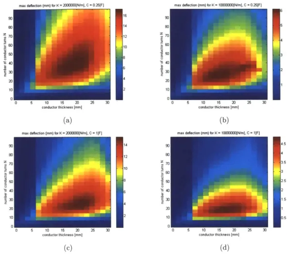
A parameter sweep that iterates the simulation across number of turns N and
con-ductor thickness y is shown in Figure 5-1. To create this figure, 25 values of N and
25 values of 7 were selected within an interesting value range. All other input
pa-rameters of the simulation were held constant at the values in Table 4. A simulation for each set of parameters was run and the maximum displacement of the formation was noted.
Symbol Description
Roi initial screen outer radius
ly conductor thickness
Wz screen axial length
N number of axial turns
p conductor resistivity
V initial capacitor voltage
C capacitor bank
capaci-tance
Resr capacitor bank effective resistance
vol capacitor to actuator vol-ume ratio
K wellbore radial spring con-stant M D Rsecr system mass wellbore damping stant SCR on resistance con-Requirement ~ 4 inches
less than 0.25 inches 12 inches
less than 30
copper: p 1.7e-8 n/m
75 V - 0.2 F
the smaller the better
1:1 desirable, do not want too large
stiff enough to be interesting, small enough that dis-placement can be measured without huge forces or obscure sensors
~10 kg
small
small
Table 5.2: Refining simulation input parameters
Description
initial screen outer radius conductor thickness screen axial length number of axial turns conductor resistivity initial capacitor voltage capacitor bank capacitance capacitor bank effective resistance capacitor to actuator volume ratio wellbore radial spring constant system mass
wellbore damping constant SCR on resistance Requirement 0.055 m sweep 0 - 12 mm 0.3 m sweep 1 - 100 turns copper: p = 1.7e-8 n/m
function of C and volume ratio sweep 0.01 to 1 F
0001 /C
1:1
sweep 106 - 107 N/r
10 kg
Table 5.3: Simulation input parameters for parameter sweep
Symbol Wz N p V C Resr vol K M D scr
6 90 16 80 14 BO 70 12 .70 E E 4 10 ts600 50 8 020 6 2 10 2 10 0 0 0 5 10 15 20 25 30 0 5 10 15 20 25 30
conductor thickness [mm] conductor thickness [mm]
(a) (b)
max deflection (mm) for K = 2(D o[N/m], C = IF] max delection (mm) for K 1E00tXM[N/ml, C = 1[F]
14 4.5 12 7 10 3.5 4 0 6702 E4 10 5 a 35 520 20 1.5 10 2 10 asM 0 0 0 5 10 15 20 25 30 0 5 10 15 20 25 30
conductor thickness [mm] conductor thickness [mm]
(c) (d)
Figure 5-1: Parameter Sweeping N and -y
Given the results of Figure 5-1 and the desired limits on N and Y - that is, desiring no more than about 25 turns of copper and no more than about 0.25 inches (6.4 mm) of conductor thickness, N can be set to 24 turns and -y set to 6.4 mm. 24 turns could easily be 25 or 26 turns; but 24 is divisible by a larger range of values, which may come in handy when discretizing the radial stiffness field (see Section 5.2.1).
Having set N and 7, the result of sweeping K and C is shown in Figure 5-2. In this figure, each vertical row (constant K, varying C) deflection result is normalized to itself; for the same force capability a formation with stiffness K = 105 N/m will have
orders of magnitude more deflection than a formation with stiffness K = 107 N/r. The first subfigure shows normalized effectiveness of the actuator for a range of C between 0.1 and 10 F, while the second subfigure refines this parameter range to 0.1
max deflection (mm) for N = 24. th = 6.4 mm 1 1.5 2 2.5 3 radial stiffness [N/m] x 07 | 1.5 2 2.5 3 radial stiffness [N/m] x Id (a) (b
Figure 5-2: Parameter Sweeping C and K
K parameter sweep
10' 10 radial stiffness [N/mI
Figure 5-3: Radial Displacement with Varying K
to 2 F because almost all of the interesting information is in this range. Though the optimal capacitance varies with K, a general choice of 0.25 F gives good performance through the K parameter sweep.
Now, a reasonable range of K can be expected given all other selected parameter values. A desired K value will result in a change in radius of more than 6 mm but less than 12 mm. Figure 5-3 shows the expected maximum displacement for the actuator system with varying K and all other parameters as specified previous in this section. A value in the range of 1 - 6 MN/m should be selected.
Finally, a rough system design for the alpha prototype is set and summarized in Table 5.4.
)
max deflection (mm) for N = 24. th = 6.4 mmSymbol Description Requirement
RO, initial screen outer radius 0.055 m
conductor thickness 6.4 mm
Wz screen axial length 0.3 m
N number of axial turns 24-26 turns
p conductor resistivity copper: p = 1.7e-8 0/m
Vo initial capacitor voltage function of C and volume ratio
C capacitor bank capacitance 0.25 F
Resr capacitor bank effective resistance .0001/C
vol capacitor to actuator volume ratio 1:1
K wellbore radial spring constant 1 - 6 MN/rn
M system mass 10 kg
D wellbore damping constant 0
Rscr SCR on resistance 0
Table 5.4: Constrained input parameters for initial prototype design
5.2
Prototype Machine Design
5.2.1
Transducer and Formation Design
The first prototype actuator system was designed around the parameter values in Table 5.4 from the previous section. This section describes the primary decisions that led to a real experimental prototype design and manufacture.
The axial conductor layout in Figure 2-3 on Page 23 shows the general conductor layout for the transducer. This layout must be mounted so that the inner coils do not move and the outer coils are constrained to only move radially outward into an experimental formation of specified stiffness. Furthermore, the experimental forma-tion must be the dominant compliance of the system so that force and displacement sensors can be fixed to a mechanical ground plane.
Simulations showed that system performance was optimized with conductor thick-nesses of 0.25 to 0.5 inches. 0.5 in thick conductors seemed too costly and hard to work with. It was decided to make the individual turns of conductor out of sheets of
0.25 in thick copper. Solid copper was chosen over stranded copper wire because
cop-per bars could provide their own radial stiffness, whereas a radial actuator that used compliant copper wire would require an additional mechanical shell around the outer
conductors for the conductors to maintain their alignment with respect to each other. As will be shown later, the second prototype used stranded wire more effectively.
Due to the high radial stiffness of the experimental formation, the frame holding the transducer, formation, and sensors should be metal (aluminum) rather than plastic. This creates an additional challenge in making sure all of the coils are electrically isolated from each other and the circuit ground plane. Thus, it is critical to mount all copper conductors to a plastic (electrically insulated) interface before connecting to the aluminum frame.
Figure 5-4 shows a cross section of the experimental frame, formation, and transducer design. Moving from the outside in, thick aluminum bars (1" x 1.5" x 12") sandwiched
by a top and bottom plate (0.25" thick) create the stiff mechanical frame for the
transducer and formation. Stiff compression springs are held between the frame and transducer by magnets. The outer loop of the transducer (the brown loop) connects to the springs via a plastic (ABS) mechanical interface. Stranded copper wire electrically connects the inner and outer conductor loops, while the inner conductor loops attach to an aluminum cylinder through another set of plastic ABS spacers. The inner aluminum cylinder is attached to the bottom aluminum plate.
Figure 5-5 shows the same cross section view of the system from an orthographic perspective. Here one can see how sets of four outer conductors (one sixth of a revolution) share an outer-frame bar and pair of springs. Additionally, at the top of the screen there are load cells in series with one set of springs.
As seen in Figure 5-4, compression springs sandwiched between magnets provide the radial stiffness required to operate the actuator system. Provided that compression springs are evenly spaced around the cylindrical transducer, the total radial stiffness is the sum of the individual spring elements:
Kradial Nsprings Kspring (5.3)
inner conductor loop
connectingwires between inner and outer conductor
outer conductor loop top plate compression spring magnet outer loop conductor-frame interface outer frame innerframe
bottom plate inner loop
conductor-frame interface
Figure 5-4: Cross section of transducer and radial stiffness
mass of the outer loop of copper bars; the one inch long springs, which are 1000 lbs/inch, could handle a few kg of cantilevered mass on their ends without deflecting in the transducer's axial direction.
#10 gauge stranded wire was used to connect inner and outer conductors together.
Three inch lengths of wire with spade terminals crimped to each end act as low stiffness mechanical flexures between the thick copper bars. Early in the design pro-cess, high stiffness blade flexures that would provide radial stiffness for the actuator and conduct current were considered; this plan was ultimately scrapped because the dimensions of a suitable flexure element were too extreme. As will be discussed in Chapter 6, the decision to use #10 gauge wire was not ideal because it contributed too much parasitic resistance. This design decision was revised in the second prototype actuator.
Figure 5-5: Orhtographic view of experimental device
loads expected by the actuator, up to 200 pounds through each spring, and also to hold all components together. 1.5" x 1" cross section bars were selected to provide sufficient surface area to create a two-bolt joint to the top and bottom plates. A justification for having both a top and bottom plate is shown in Figure 5-6. Both FEA results have 800 N loads along each contact area between the spring and bar; the cantilevered beam deflects nearly 0.3 mm, while the top and bottom plate fixed bar deflects only
0.003 mm in this loading scenario. 0.3 mm could approach a percentage of the total
spring deflection, while 0.003 mm would be barely 0.01% of total deflection.
Specifying compression load cells was fairly easy at this load requirement and size scale. The load cells are 250 pound max cells from Omega; one mounts in series with a spring on one of the six bars. The plastic connectors that provide electrical isolation for the copper bars are shown in Figure 5-7. The plastic pieces and copper bars are water jetted and epoxied together on the joint.
URES (mm) 3.479e-003 3.189e-003 2 899e-003 2.609e-003 2.3198-0 2.029e4)03 1.739e-003 1.450e-003 1.180e-003 8.697e-004 5.798e-004 2.899e-004 I 0008-030
(a) Top and Bottom Fixed Bar
LRES (mm)
3.1778-001
2.912e-001 2.647e-001 2.383e-00 2.118e-001 1.853e-001 1.588e-001 1.324e-001 1.059e-001 7.942e-002 5.295e-002 2.647e-002 1.000e-030(b) Bottom Fixed Bar
Figure 5-6: FEA result for 800N loads on each spring
(a) outer conductor plastic feature (b) inner conductor plastic feature
Figure 5-8: Completed Alpha Prototype Transducer, Formation, and Capacitor Bank The completed transducer is shown in Figure 5-8. Similarly, the complete experimen-tal system including charging circuit, power circuit, and data acquisition system is shown in Figure 5-9.
5.2.2
Capacitor Bank and Circuit Components
Building a 0.25 F, 75 V capacitor bank by hand is most practically done using large aluminum electrolytic capacitors. Other capacitor types are more practical for han-dling extreme environment operation and for decreasing ESR, but aluminum