HAL Id: hal-00112147
https://hal.archives-ouvertes.fr/hal-00112147
Preprint submitted on 8 Nov 2006
HAL is a multi-disciplinary open access
archive for the deposit and dissemination of
sci-entific research documents, whether they are
pub-lished or not. The documents may come from
teaching and research institutions in France or
L’archive ouverte pluridisciplinaire HAL, est
destinée au dépôt et à la diffusion de documents
scientifiques de niveau recherche, publiés ou non,
émanant des établissements d’enseignement et de
recherche français ou étrangers, des laboratoires
Mathematical analysis of
Khokhlov-Zabolotskaya-Kuznetsov (KZK) equation
Anna Rozanova-Pierrat
To cite this version:
Anna Rozanova-Pierrat. Mathematical analysis of Khokhlov-Zabolotskaya-Kuznetsov (KZK)
equa-tion. 2006. �hal-00112147�
Mathematical analysis of
Khokhlov-Zabolotskaya-Kuznetsov (KZK)
equation
Anna Rozanova-Pierrat
∗September 13, 2006
AbstractWe consider the Khokhlov-Zabolotskaya-Kuznetzov (KZK) equation
(ut− uux− βuxx)x− γ∆yu= 0, which describes for instance the
propa-gation of sound beams in nonlinear media, in Sobolev spaces of functions periodic on x and with mean value zero. The derivation of KZK from the non linear isentropic Navier Stokes and Euler equations and approxima-tion their soluapproxima-tions (in viscous and non viscous cases), the results of the existence, uniqueness, stability and blow-up of solution of KZK equation (using Alinhac’s method) are obtained. We proved the existence of the shock wave for the problem with β = 0 (without viscosity and dissipation of energy). We have established the global existence in time of the beam’s propagation in viscous media with β > 0 only for rather small initial data. In the proof of the existence of KZK solution the fractional step method have been analyzed. One justifies and gives as an example the numeri-cal results of Thierry Le Poll`es obtained by him in Laboratoire Ondes et Acoustique, ESPCI, Paris.
1
Introduction
The KZK equation, named after Khokhlov, Zabolotskaya and Kuznetsov, was originally derived as a tool for the description of nonlinear acoustic beams (cf for instance [10, 39]). It is used in acoustical problems as mathematical model that describes the pulse finite amplitude sound beam nonlinear propagation in the thermo-viscous medium, see for example [1, 24, 8, 9, 27]. Later it has been used in several other fields and in particular in the description of long waves in ferromagnetic media [33].
The KZK equation, as it have been demonstrated in [8], accurately describes the entire process of self-demodulation throughout the near field and into the far field, both on and off the axis of the beam (in water and glycerin). The
term “self-demodulation”, which was coined in the 1960s by Berktay, refers to the nonlinear generation of a low-frequency signal by a pulsed, high-frequency sound beam.
As it is known [9], the use of intense ultrasound in medical and industrial applications has increased considerably in recent years. Both plane and focused sources are used widely in either continuous wave or pules mode, and at in-tensities which lead to nonlinear effects such as harmonic generation and shock formation. Typical ultrasonic sources generate strong diffraction phenomena, which combine with finite amplitude effects to produce waveforms that vary from point to point within the sound beam. Nonlinear effects have become es-pecially important at acoustic intensities employed in many current therapeutic and surgical procedures. In addition, biological media can introduce significant absorption of sound, which must also be considered. The KZK equation, as a nonlinear equation with effects of diffraction and of absorption, which can provide shock formation, is the mathematical model of these phenomena.
The non-linear phenomena found a recent application in the field of the ultra-sonic medical imagery known under the name of “harmonic imagery”. In med-ical imagery where the echographic bars concentrates energy in a very narrow beam, the approach most commonly employed is the resolution of the equation KZK which describes focused beams.
In the present section the emphasis is put on the derivation of the equa-tion for nonlinear acoustic in view of applicaequa-tion to time reversal problems in nonlinear media. The KZK equation in its initial interpretation as in [10] is mostly studied by physicists but until now there are is no mathematical analy-sis of this problem. The KZK equation is not an integrable equation at variance Kadomtsev-Petviashvili (KP) equation known to be integrable. Numerically in [10] has been obtained the existence of a shock wave in the case of propagation of the beam in nondissipative media and a quasi shock wave for the dissipative media. The last phenomenon corresponds to the approximation of the beam’s front to the shock wave but the solution has the tentative to be global. We obtained the proof of the existence of the shock wave for the problem without viscosity. We have established the global existence in time of the propagation in viscous media only for rather small initial data. The announcement of the results can be found in [11, 12, 13].
This part is organized in the following way. First the derivation of the equation is borrowed from physical literature then the existence uniqueness stability of the equation is analyzed. Eventually a blow-up result which gives a limitation to the range of application is given as an adaptation of a result of [2], [3] and [4]. Using obtained results one proves a large time validity of the approximation for two cases: for non viscous thermoellastic media and viscous thermoellastic media.
Our main purpose is to prove existence and stability of solutions described by the KZK equation with the following properties
1. they are concentrated near the axis x1;
3. they are generated either by initial condition or by a forcing on the bound-ary x1= 0.
This corresponds to the description of the quasi one d propagation of a signal in an homogenous but nonlinear isentropic media.
Therefore it is assumed that its variation in the direction x′ = (x
2, x3, . . . , xn)
perpendicular to the x1 axis is much larger that its variation along the axis x1.
For instance for the linear wave equation in Rn (n > 1):
1 c2∂
2
tu − ∆u = 0 , (1)
the following ansatz
uǫ= U (t − x1 c , ǫx1, √ ǫx′) (2) involving a “profile” U (τ, z, y) (with ǫ) small leads to the formula:
∂2 τ,zU −
1
2∆yU = O(ǫ), (3) or for functions U (τ, z, y) = A(z, y)eiωτ, to the equation
iω∂zA −
1
2∆yA = O(ǫ). (4) Observe that with ǫ = 0 (3) and (4) are two variants of the classical paraxial approximation and that equation (3) contains the linear non diffusive terms of the KZK equation which usually has the following form for some positive constants β and γ: ∂τ,z2 U − 1 2∂ 2 τU2− β∂τ3U − γ∆yU = 0.
On the other hand the isentropic evolution of a thermo-elastic non viscous media is given by the following Euler Equation:
∂tρ + ∇(ρv) = 0 , ρ(∂tv + v · ∇v) = −∇p(ρ) . (5)
Any constant state (ρ0, v0) is a stationary solution of (5). Linearization near
this state introduces the variables
ρ = ρ0+ ǫ˜ρ , v = v0+ ǫ˜v
and the acoustic system:
which is equivalent to the wave equation: 1 c2∂ 2 tρ − ∆˜˜ ρ = 0 , ∂t˜v = −p ′(ρ 0) ρ0 ∇˜ ρ, (7) where c =pp′(ρ
0) is the sound speed of the unperturbed media.
And observe that the equation (3) which is the linearized and non viscous part of the KZK equation can be obtained in two steps. First consider small perturbations of a constant state for the isentropic Euler equation which are solution of the acoustic equation and then consider a paraxial approximation of such solutions.
The derivation of the full KZK equation follows almost the same line. It takes into account the viscosity and the size of the nonlinear terms. One starts from a Navier Stokes system:
∂tρ + ∇(ρu) = 0 , ρ[∂tu + (u · ∇) u] = −∇p(ρ, S) + b∆u , (8)
the pressure is given by the state law p = p(ρ, S), where S is entropy.
First one assumes that the temperature T and the entropy S have the small increments ˜T and ˜S. With the hypothesis of potential motion one introduces constant states
ρ = ρ0, u = u0.
Next one assumes that the fluctuation of density (around the constant state ρ0), of velocity (around u0, which can be taken equal to zero with galilean), are
of the same order ǫ:
ρǫ= ρ0+ ǫ˜ρǫ, uǫ= ǫ˜uǫ, b = ǫ˜b,
here ǫ is a dimensionless parameter which characterizes the smallness of the per-turbation. For instance in water with a initial power of the order of 0.3 Vt/cm2
ǫ = 10−5. Using the transport heat equation in the form
ρ0T0
∂ ˜S
∂t = κ△ ˜T , the approximate state equation
p = c2ǫ˜ρǫ+ 1 2 µ∂2p ∂ρ2 ¶ S ǫ2ρ˜2ǫ+ µ∂p ∂S ¶ ρ ˜ S
(where the notation (·)S means that the expression in brackets is constant on
S), can be replaced [10], thanks to the relation ˜ S = −κ T0 µ∂T ∂p ¶ S div uǫ, by p = c2ǫ˜ρǫ+(γ − 1)c 2 2ρ0 ǫ2ρ˜2ǫ− κ µ 1 Cv − 1 Cp ¶ ∇.uǫ. (9)
The system (8) becomes an isentropic system
∂tρǫ+ ∇(ρǫuǫ) = 0 , ρ[∂tuǫ+ (uǫ· ∇) uǫ] = −∇p(ρǫ) + ǫν∆uǫ, (10)
with the approximate state equation
p = p(ρǫ) = c2ǫ˜ρǫ+(γ − 1)c 2
2ρ0
ǫ2ρ˜2
ǫ (11)
and a rather small and positive viscosity coefficient:
ǫν = b + κ µ 1 Cv − 1 Cp ¶ .
Next one reminds the direction of propagation of the beam say along the axis x1, and therefore considers the following profiles:
˜ ρǫ= I(t − x1 c , ǫx1, √ ǫx′) , (12) ˜ uǫ= (uǫ,1, u′ǫ) = (v(t − x1 c , ǫx1, √ ǫx′),√ǫ ~w(t − x1 c , ǫx1, √ ǫx′)) . (13)
In (12) and (13) the argument of the functions will be denoted by (τ , z , y) and c is taken equal to the sound speed c =pp′(ρ
0) . Inserting the functions
ρǫ= ρ0+ ǫI, uǫ in the system (10) one obtains:
1 For the conservation of mass: ∂tρǫ+ ∇(ρǫuǫ) = ǫ(∂τI − ρ0 c ∂τv) + +ǫ2 Ã ρ0(∂zv + ∇y· ~w) − 1 cv∂τI − 1 cI∂τv ! + O(ǫ3) = 0 . (14)
2 For the conservation of momentum in the x1 direction:
ρǫǫ(∂tuǫ,1+ uǫ∇uǫ,1) + ∂x1p(ρǫ) − ǫ 2ν∆u ǫ,1= ǫ(ρ0∂τv − c∂τI) + +ǫ2 Ã I∂τv −ρc0v∂τv + c2∂zI −(γ−1)2ρ0 c∂τI2−cν2∂τ2v ! + O(ǫ3) = 0. (15)
And finally for the orthogonal (to the axis x1) component of the momentum
one has: ρǫǫ(∂tu′ǫ+ uǫ∇u′ǫ) + ∂x′p(ρǫ) − ǫ2ν∆u′ ǫ= ǫ 3 2(ρ0∂τw + c~ 2∇yI) + +ǫ52(−ρ0v c ∂τw + I∂~ τw +~ (γ−1)c2 2ρ0 ∇yI 2− ν c2∆yw) + O(ǫ~ 3) = 0. (16)
To eliminate the terms of the first order in ǫ we need to pose: ∂τI −ρ0
which also implies
ρ0∂τv − c∂τI = 0,
and therefore I and v should be related by the formula: v = c
ρ0
I (18)
and the second order terms of (14) and (15) by the formula: ρ0(∂zv + ∇y· ~w) −c1v∂τI −1cI∂τv = = −1c(I∂τv − ρ0 c v∂τv + c2∂zI − (γ−1) 2ρ0 c∂τI 2− ν c2∂τ2v), (19)
which (with (18)) gives:
ρ0∇y· ~w + 2c∂zI − (γ + 1) 2ρ0 ∂τI2− ν c2ρ 0 ∂τ2I = 0. (20)
Eventually one uses the equation of the orthogonal moment (16) to eliminate the term ρ0∇y· ~w. Assume in agreement with (16) that
ρ0∂τw + c~ 2∇yI = 0, (21)
take the divergence with respect to y of this equation. Differentiate (20) with respect to τ , and combine to obtain:
c∂τ z2 I − (γ + 1) 4ρ0 ∂τ2I2− ν 2c2ρ 0 ∂τ3I − c2 2∆yI = 0. (22) The KZK equation (22) is written for the perturbation of density, but the same equation with only different constants can be also derived for the pressure and the velocity. The passage between these KZK equations is possible thanks to (11), (18) and (21). For example the equation for the pressure has the form
∂2 τ zp − β 2ρ0c3 ∂2 τp2− δ 2c3∂ 3 τp − c 2△yp = 0.
The above derivation is standard in physic articles however it does not imply that the function
ρǫ= ρ0+ ǫI, uǫ= ǫ(v,√ǫ ~w)
is a solution of the system (10) with an error term of the order of ǫ3. In fact
one can assume (17) and that (21) with (20) take place, but not the fact that this quantity which corresponds to the term of the order of ǫ2 both in the
conservation of mass and momentum along the axis x1 is zero. To remedy to
this fact and also to ensure an error of the order of ǫ52 in the moment orthogonal
to the x1 direction one introduces an Hilbert expansion type construction and
writes
assuming that I is solution of the KZK equation (22), while v and w are given in term of I by (18) and (21), one obtains, modulo terms of order ǫ52, for the
right hand side of the equations (14), (15) and (16):
ǫ2 Ã −ρc0∂τv1+ ρ0(∂zv + ∇y· w) − 1 ρ0 ∂τI2 ! , ǫ2 Ã ρ0∂τv1+ c2∂zI −γ − 1 2ρ0 c∂τI 2 −cρν 0∂ 2 τI ! .
Taking into account the KZK equation this implies for the “corrector” v1 the
relation: ∂τv1=γ − 1 2ρ2 0 c∂τI2+ ν cρ2 0 ∂τ2I − c2 ρ0 ∂zI. (24)
At this point one can state a theorem with hypothesis to be specified later in section 3 (see theorems 7,8, 10).
Theorem 1 Let I be a smooth solution of the KZK equation (22), define the functions v, w and v1 by the known I. Define the function Uǫ= (ρǫ, uǫ) by the
formula: (ρǫ, uǫ)(x1, x′, t) = (ρ0+ ǫI, ǫ(v + ǫv1,√ǫ ~w))(t − x1 c , ǫx1, √ ǫx′).
Then there exist constants C ≥ 0 and T0= O(1), such that for any finite time
0 < t < T01ǫln1ǫ and ǫ > 0, there exists a smooth solution Uǫ= (Rǫ, Uǫ)(x, t) of
the isentropic Navier-Stokes equation such that one has for some s ≥ 0: kUǫ− UǫkHs≤ ǫ
5 2eǫCt.
It is interesting to notice that for the non viscous case, i.e., for the isentropic compressible Euler system, the KZK like equation with β = 0 have been ob-tained using the scaling of nonlinear diffractive geometric optic theory in [16, p. 1233] (in 2d) in the framework of nonlinear diffractive geometric optic with rec-tification. The initial goal of the article is to construct the nonlinear symmetric hyperbolic equation
L(u, ∂x)u + F (u) = 0,
and the case of the isentropic compressible Euler system is given as an example. The basic ansatz in [16] has three scales
uǫ(x) = ǫ2a µ ǫ, ǫx, x,x · β ǫ ¶ , where a(ǫ, X, x, θ) = a0(X, x, θ) + ǫa1(X, x, θ) + ǫ2a2(X, x, θ).
Here x = (t, y) ∈ R1+d, β = (τ, η) ∈ R1+d and the profiles a
j(X, x, θ) are
periodic in θ. The KZK like equation of the form ∂Ta − △y∂θ−1a + σa∂θa = 0,
with σ ∈ R determined from some identity and with T = tǫ, holds for the
profile a0 with mean value zero on θ (for the proof see [16, pp. 1231, 1234])
which corresponds to vanishing non oscillatory part, if we have in our mind the notation of [16, p.1181]:
if (see [16, p.1181]) a := 2π1 R02πadθ, the oscillating part is denoted a∗ :=
a − a.
The analogue technique is used in [38] to study the short wave approximation for general symetric hyperbolic systems as
½
L(∂)u = ˜F (u)∂xu, with (x, y) ∈ R × R,
u(0) = ǫu0(x/ǫ, y) ∈ Rn. (25)
with an hyperbolic operator L(∂) = ∂t+ A∂x+ B∂y+ E. Short waves stands
for short-wavelenght approximate solutions, or equivalently approximate solu-tions with initial data whose oscillatory frequencies are large compared to the paremeters of the system. For the variables
T =t ǫ, X =
x
ǫ, y, τ = ǫt (26) in [38] one looks for the approximate solutions in the form
uǫ(t, x, y) = ǫ(u0+ ǫu1+ ǫ2u2)(T, X, y, τ ).
For the first profile u0one has the system of the form
½
(∂T+ c∂X)u0= 0,
(∂τ∂X− ∂2Y)u0= ∂X(u0∂Xu0). (27)
corresponding to the KZK equation for the function ˜u0(X −cT, τ, y, X). The
estimate of the approximate result in [38] between the exact solution vǫ of (25)
and the solution uǫ
0of a system of the form (27) is following
1 ǫkv
ǫ
− ǫuǫ0kL∞([0,τ0/ǫ]×R2x,y)= o(1).
To analyze common points between this work and KZK-approximation we can pass from the variables corresponding to our scaling
(t − xc1, ǫx1,√ǫx′)
to “ ^variable =√ǫ variable” in following way µ 1 √ ǫ(˜t − ˜ x1 c ), √ ǫ˜x1, ˜x′ 
and supposing now that ǫ = ˜ǫ2, i.e., we obtain µ1 ˜ ǫ(˜t − ˜ x1 c ), ˜ǫ˜x1, ˜x ′ ¶ , and similar (ρ, u) = (ρ0+ ˜ǫ ˜I, ˜ǫ(˜v + ˜ǫ2˜v1, ˜ǫ ˜w)).
This variables exactly correspond to Texier’s case [38] (T −Xc , τ, y).
To the first profile ǫu0 from [38] there corresponds to (ρ0+ ˜ǫ ˜I, ˜ǫ˜v) for which
we have exactly the system (27) in the form of (17) and the KZK equation without viscous therm. The profile ˜ǫ2w is associated to ǫ˜ 2u
1 and the profile
˜ ǫ3v˜
1 is associated to ǫ3u2. The result of [38] is obtained for nonperiodic case
and without the vanishing mean condition important for physical reasons. This small analysis of the abstract works shows that our approach is simi-lar where the variables have been switched with ǫ “ ^variable = √ǫ variable” to balance the oscillation :
1 √ ǫ µ ˜ t − x˜c1 ¶ 7→³t −xc1´.
In other words we can say that we have O(1) oscillations.
The scaling of Sanchez [33] for Landau-Lifshitz-Maxwell equations in R3 is
very different. Sanchez starts by the system ∂tM = −M ∧ H − γ |M|M ∧ (M ∧ H) in R 3, (28) ∂t(H + M ) − ∇ ∧ E = 0 in R3, (29) ∂tE + ∇ ∧ H = 0 in R3, (30)
which represents the Landau-Lifshitz-Maxwell equations and admits stable equi-librium solutions where the magnetization is uniform and everywhere parallel to the effective magnetic field:
(M, H, E)α= (M0, α−1M0, 0), α > 0. (31)
Then he is interesting in small perturbations of the equilibrium states whose size is measured by a small parameter ǫ. The perturbation is taken in the form:
M (t, x, y) = M0+ ǫ2M (˜ft, τ, ˜x, ˜y),
H(t, x, y) = α−1M
0+ ǫ2H(˜e t, τ, ˜x, ˜y),
E(t, x, y) = ǫ2E(˜e t, τ, ˜x, ˜y), where ˜t, τ, ˜x, ˜y are new rescaled variables:
˜
We notice here that if we take ˆ
t = ǫ3t, ˆx = ǫ3x, ˆy = ǫ3y, we exactly obtain (26) from (32):
˜ t = ˆt ǫ, τ = ǫˆt ˜x = ˆ x ǫ, ˜y = ˆy.
But the smallness of the functions’ profiles are different. The vector of pertur-bation U (˜t, τ, ˜x, ˜y) =³α−1
2M , ef H, eE
´t
(˜t, τ, ˜x, ˜y) satisfy an equation in the form ( ∼ on the variables is omitted)
∂tU + ǫ2∂τU + A1∂xU + ǫA2∂yU + ǫ−2LU = B(U, U ) + ǫ2T (U, U, U ),
U (0, 0) = U0 0,
where A1, A2, L are linear operators in R9, B is a bilinear map on R9×R9, and
T is a trilinear map on R9×R9×R9. Using then an asymptotic formal expansion
of U in the form U ≡ U0+ ǫU1+ ǫ2U2+ ..., Sanchez obtains that the leading
term U0breaks down in five traveling and standing terms, U0=P5j=1uj, which
satisfy the transport equation and the Zabolotskaya-Khokhlov equation: (∂t+ vj∂x)uj= 0,
∂x(∂τuj− Dj∂x2uj+ Bj(uj, ∂xuj) + Fj(uj, uj, uj)) = Cj∂y2uj
with constant vj which is the speed of the wave in the direction k (the
x-direction). He also proves the validation of this approximation for the time of order T0
ǫ2.
Remark 1 Several limits of the equation (37) leads to classical PDE. • With ρ0c → ∞ it becomes the paraxial approximation:
∂2τ zI −
c
2∆yI = 0, (33) or in term of the pressure the equation
∂p ∂z = c 2 Z τ 0 △ ypdτ′.
The solutions of these equations have been numerically computed by Thierry Le Poll`es (in Laboratoire Ondes et Acoustique, ESPCI, Paris) using a fractional step method. The proof of the validity of this method will be given in section 2.1.2. The figures 2 and 3 have been simulated for the three dimensional problem for pressure p of a sound beam propagating in the water
∂p ∂z = c 2 Z τ 0 △ ypdτ′, y = (y1, y2),
p(τ, 0, y) = g(τ ) y ∈ Ω, τ > 0, ∂p
∂n= 0 for ∂Ω, τ > 0. Here g(τ ) is the signal of the source situated in z = 0 and
g(τ ) = P0exp[−(2τ/Td)2m] sin(w0t). (34)
• And when I does not depend on y it is the Burgers-Hopf equation
c∂zI −(γ + 1) 4ρ0 ∂τI2− ν 2c2ρ 0 ∂τ2I = 0 (35)
and eventually in this case with ν = 0 the Burgers equation:
c∂zI −
(γ + 1) 4ρ0
∂τI2= 0.
In term of the pressure fluctuation, (35) is ∂p ∂z = δ 2c3 ∂2p ∂τ2 + β 2ρ0c3 ∂p2 ∂τ2. (36)
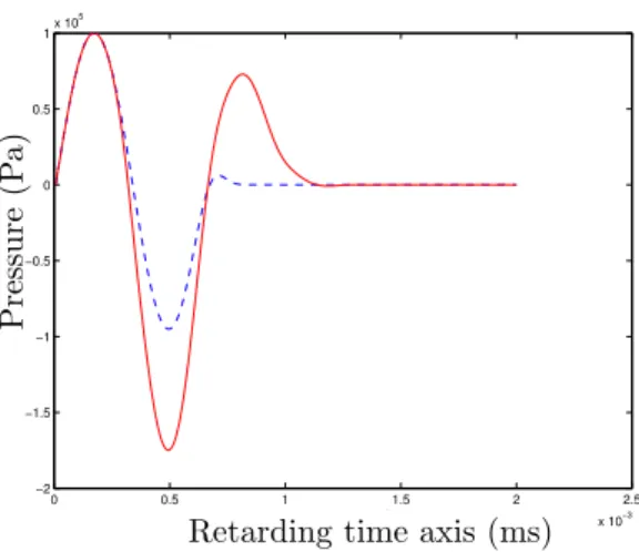
The numerical simulation of the solution of (36) with the same initial and bound-ary data as in (33) is given in the figures 4 and 5.
• The analogous 2d version of KZK equation is
c∂τ z2 I − (γ + 1) 4ρ0 ∂ 2 τI2− ν 2c2ρ 0∂ 3 τI − c2 2∂ 2 yI = 0.
And for a “beam” (rotationally invariant around the x1axis) in 3 space variables
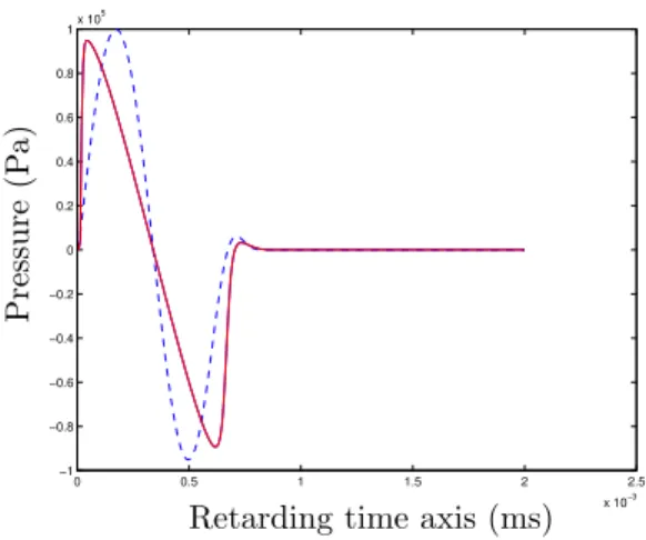
it is: c∂2τ zI − (γ + 1) 4ρ0 ∂2τI2− ν 2c2ρ 0 ∂3τI − c2 2(∂ 2 rI + 1 r∂rI) = 0. (37) The figures 6 and 7 represent the graph of the solution of the full KZK equation, composed of the both parts of (33) and (36) with the source (34)
∂p ∂z = c 2 Z τ 0 △ ypdτ′+ δ 2c3 ∂2p ∂τ2 + β 2ρ0c3 ∂p2 ∂τ2. (38)
All figures 2-7 have been obtained by Thierry Le Poll`es in Laboratoire Ondes et Acoustique, ESPCI, Paris, and are the illustrations of his numerical results calculated in C++.
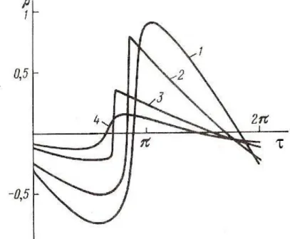
Remark 2 We would like also illustrate the case of “quasi-shock” using [10, pp.78-81]. This phenomenon appears for the KZK equation with small viscosity coefficient. According to [10] the wave is named a quasi shock wave if the breadth of the wave front △τ ≤ π/10. The figures 8 and 9 have been obtained in [10] for
the following problem for the density function of a beam rotationally invariant around the x1 axis (cf. (37))
∂2ρ2 ∂τ ∂z− N ∂2ρ2 ∂τ2 − δ ∂3ρ ∂τ3− µ ∂2 ∂r2 + 1 r ∂ ∂r ¶ ρ = 0, (39) ρ|z=0= −e−r 2 sin τ.
Remark 3 There are mathematical works [25], [26] for KZK type equation αuzτ = (f (uτ))τ+ βuτ τ τ + γuτ+ △xu,
where uτ = uτ(z, x, τ ) is the acoustic pressure, (z, x) ∈ Rd× R, d = 1, 2 are
space variables and τ is the retarded time. The equation is studied with the hypothesis that the nonlinearity f has bounded derivative which allows to proof the global existence for the case when the coefficients are rapidly oscillating functions of z. So this problem is not related with our “acoustical” problem for the KZK equation where as we will see later there is a blow-up result illustrating the existence of a shock wave.
2
Mathematical Studies of the Cauchy Problem
for KZK Equation
2.1
Existence uniqueness and stability of solutions of the
KZK equation
Following the mathematical tradition in this section and in the next one the unknown will be denoted by u, and the variables (x, y) ∈ Rx× (Ω ⊆ Rn−1).
When Ω 6= Rn−1 it is assumed that the solution satisfies on its boundary the
Neumann boundary condition. Multiplying u by a positive scalar one reduces the problem to an equation involving only two constants β and γ
(ut− uux− βuxx)x− γ∆yu = 0 in Rx/(LZ) × Ω. (40)
For sake of simplicity and because this also corresponds to practical sit-uations [10, 39] we consider solutions which are periodic with respect to the variable x and which are of mean value zero:
u(x + L, y, t) = u(x, y, t), Z L
0
u(x, y, t)dx = 0. (41)
Observe that the conditions (41) are compatible with the flow and that the second one is “natural” because we consider fluctuations.
For these functions the norm of the space Hs(s ∈ R, s ≥ 0) is denoted by
kukHs = Z Rn−1 +∞ X k=−∞ (1 + k2+ η2)s|ˆu(k, η)|2dη 1 2 .
If we introduce the operator Λ = (1 − ∆)12 as [(Λu)(ζ) = (1 + |ζ|2) 1 2u(ζ),ˆ
then
Λs= (1 − ∆)s2, kukHs = kΛsukL2. (42)
We define the inverse of the derivative ∂−1
x as an operator acting in the space
of periodic functions with mean value zero this gives the formula:
∂x−1f = Z x 0 f (s)ds + Z L 0 s Lf (s)ds. (43) This form of the operator ∂−1
x preserves the both qualities: the periodicity and
having the mean value zero.
In this situation equation (40) is equivalent to the equation
ut− uux− βuxx− γ∂x−1∆yu = 0 in Rx/(LZ) × Ω. (44)
Finally when γ = 0 equation (40) reduces to the Burgers-Hopf equation for which existence smoothness and uniqueness of solution are well known. For γ = β = 0 it reduces to the Burgers equation
∂tu − ∂xu 2
2 = 0,
which after a finite time exhibits singularities. After this “blow-up” time the solution can be uniquely continued into a weak solution satisfying an elementary entropy condition (in the present case with γ 6= 0 it seems that this construction cannot be adapted to equation (40) with β = 0 and γ 6= 0).
We would like also to notice that the J. Bourgain-type method and introduc-tion the Bourgain spaces as in [35, 29, 30] and others are not useful for the KZK problem because of absence of the terms with an odd derivative as for example uxxx in (44). The presence only of the second derivative make impossible the
main estimations and equalities of this method.
2.1.1 A priori estimates for smooth solutions
According to the standard approach we first establish a priori estimates for smooth solutions which are in particular a consequence of the relation:
Z L 0 Z Rn−1y ∂x−1(∆yu)udxdy = − Z L 0 Z Rn−1y ∂x−1(∇yu)∇yudxdy = Z L 0 Z Rn−1 y ∂−1 x (∇yu)∂x(∂x−1(∇yu))dxdy = 0. (45)
The L2norm and the Hsin (R+x/(LZ)) × Rn−1y ) are denoted by |u| and by
Proposition 1 The following estimates are valid for solutions of the integrated KZK equation (44): 1 2 d dt|u(·, ·, t)| 2 + β|∂xu(·, ·, t)|2= 0 , (46) For s > [n 2] + 1 1 2 d dtkuk 2 s+ βk∂xuk2s≤ C(s)kuk3s (47) and 1 2 d dtkuk 2 s+ βC(L)kuk2s≤ C(s)kuk3s. (48)
The estimates (47), (48) are valid for s > [n2]+1 which is the necessary condition because of application of the Sobolev theorem.
Proof. To obtain the relation (46) multiply (44) by u, and integrate by part. It shows that for β = 0 we have the conservation law for the norm of u in L2(R+x/(LZ)) × Rn−1y ). If β > 0 we also have according to the physical
phe-nomena [10] the dissipation of energy.
For the clarity the proof of (47) is done firstly in 3 space variables, with Ω = R2 and s an integer (i.e. in the present case s = 3) and after we give the
proof in general case. In 2d in particular when Ω = S1the proof is even simpler.
The proof in the whole is similar except for the relation (48) which holds only in the periodic case and not on the whole line. (In this later case the Hsnorm
of ∂xu does not control the Hsnorm of u).
For the proof of general case s ∈ R one has used the representation of the norm in Hs with the help of the operator Λ by (42) and the technique
demonstrated in [23] and [34] for periodic and nonperiodic cases, which allows to deduce 1 2 d dtkuk 2 s+ βk∂xuk2s≤ Ck∇x,yukL∞kuk 2 s,
and this implies the necessity of our restriction for s: if s > [n
2] + 1 then H
s−1
⊂ L∞.
The elementary proof
The introduction of the H3 norm for n = 3 comes from the control of the
nonlinearity with the Sobolev theorem. It starts with the estimating Z L
0
Z
R2 y
∂x3(u∂xu)∂x3udxdy. (49)
We integrate it by parts, use the x periodicity, and finally one has:
| Z L 0 Z R2 y
∂3x(u∂xu)∂x3udxdy| ≤ C|∂xu|L∞
(]0,L[,×R2 y)kuk
2 H3(R
In the same way with ∂ydenoting the derivative with respect to any orthogonal
component one obtains: Z L
0
Z
R2 y
∂3y(u∂xu)∂y3udxdy =
Z L 0
Z
R2 y
u∂x(∂y3u)∂y3udxdy +
Z L 0 Z R2 y (∂y3u)2∂xudxdy + +3 Z L 0 Z R2 y
(∂yu)(∂y2∂xu)∂y3udxdy + 3
Z L 0
Z
R2 y
∂y2u(∂y∂xu)∂y3udxdy (50)
and as above one has Z L 0 Z R2 y u∂x(∂3yu)∂y3u = − 1 2 Z L 0 Z R2 y ∂xu(∂3yu)2dxdy.
Therefore the sum of the first, second and last term of (50) are bounded by C|∂yu|L∞(]0,L[×R2
y)kuk
2
H3(]0,L×R2 y)
and for the third term one can write: Z L
0
Z
R2 y
∂2yu(∂y∂xu)∂y3udxdy =
1 2 Z L 0 Z R2 y ∂y(∂y2u)2(∂y∂xu)dxdy = −12 Z L 0 Z R2 y (∂y2u)2∂x(∂y2u)dxdy = 0.(51)
Finally one has obtained the following estimate: Z L 0 Z R2 y (∂x3(u∂xu)(∂x3u) + X 1≤i≤2 ∂y3i(u∂xu)(∂ 3 yiu))dxdy ≤ ≤ (sup
x,y |∂xu(x, y, t)| + |∇yu(x, y, t)|)kuk 2
3. (52)
The choice of the index of derivation 3 comes from the Sobolev theorem which gives:
|∂xu| + |∂yu| ≤ CkukH3(]0,L[×R2 y).
Eventually to obtain (47) write:
0 = Z L 0 Z R2 y [∂3
x(ut− uux− βuxx− γ∂−1x ∆yu(s, y)ds).∂x3u
+ X
1≤i≤2
∂y3i(ut− uux− βuxx− γ∂
−1
x ∆yu(s, y)ds).∂y3iu]dxdy
and use the estimate (52). Finally to prove (48) one uses the fact that u is of x mean value 0 and therefore it is (cf: (43)) related to ∂xu by the formula
u = ∂x−1∂xu = Z x 0 ∂xu(s, y)ds + Z L 0 s L∂xu(s, y)ds, (53)
which implies the relation
kukH3(]0,L[×R2
y)≤ Ck∂xukH3(]0,L[×R2y).
The general proof
We apply the operator Λs to equation (44) and multiply by Λsu in L 2 1 2 d dtkuk 2 Hs− β(Λsuxx, Λsu) − (Λs(uux), Λsu) = 0, 1 2 d dtkuk 2 Hs+ βkuxk2Hs− (Λs(uux), Λsu) = 0.
Suppose that [Λs, u]v = Λs(uv) − uΛsv. Then
(Λs(uux), Λsu) = ([Λs, u]ux, Λsu)+(u∂xΛsu, Λsu) = ([Λs, u]ux, Λsu)−1
2(uxΛ
su, Λsu).
As soon as 2(s − 1) > n, the last term is estimated by |(uxΛsu, Λsu)| ≤ kuxkL∞kuk
2
Hs ≤ CkuxkHs−1kuk2Hs ≤ Ckuk3Hs.
For the first term we have:
([Λs, u]ux, Λsu) ≤ k[Λs, u]uxkL2kukHs ≤ CkukHskuxkHs−1kukHs ≤ Ckuk
3 Hs.
We need now the following proposition.
Proposition 2 With the above notations we have the estimate k[Λs, u]uxkL2 ≤ CkukHskuxkHs−1.
Proof.
For the periodic case, using the result of J.C. Saut and R. Temam from [34] which consists in the following:
if u, v are in Hs(Rn) or in Hs(Rn/Zn) and s ∈ R, s > 1, γ ∈ R, γ > n/2,
then
kDs(uv) − uDsvk
L2≤ c(γ, s){kukskvkγ+ |ukγ+1kvks−1},
what is easy to generalize for Hs(R
x/(LZ))×Rn−1y . The estimate remains true
if we change Dson Λs.
In our case γ = s − 1, from where the result follows. ¤ To finish the proof for (48) we notice that kukHs ≤ Ck∂u
∂xkHs, because of
2.1.2 Existence and uniqueness for smooth solutions
The following theorem is an easy consequence of the a priori estimates. Theorem 2 For the following Cauchy problem
ut− uux− βuxx− γ∂x−1(∆yu) = 0 , u(x, y, 0) = u0 (54)
considered in (Rx/(LZ)) × Rn−1y , i.e. in the class of x periodic functions with
mean value 0 with the operator ∂−1
x defined by the formula (43) and finally with
β ≥ 0 one has the following results. 1 For s > [n
2] + 1 (s = 3 for instance in dimension 3) there exists a constant
C(s, L) such that for any initial data u0 ∈ Hs the problem (54) has on an
interval [0, T [ with
T ≥ 1
C(s, L)ku0kHs (55)
a solution in C([0, T [, Hs) ∩ C1([0, T [, Hs−2).
2 Let T∗ be the biggest time on which such solution is defined then one has
Z T∗
0
sup
x,y(|∂xu(x, y, t)| + |∇yu(x, y, t)|)dt = ∞.
(56)
3 If β > 0 there exists a constant C1 such that
ku0ks≤ C1⇒ T∗= ∞. (57)
4 For two solutions u and v of KZK equation, assume that u ∈ L∞([0, T [; Hs), v ∈ L2([0, T [; L2). Then one has the following stability
unique-ness result:
|u(, t) − v(., t)|L2≤ e
Rt
0supx,y|∂xu(x,y,s)|ds|u(., 0) − v(., 0)|L2. (58)
Remark 4 The estimate (58) is of strong-weak form, as in [14] only the L∞
norm of ux is needed.
Remark 5 When there is no viscosity all the corresponding statements of the theorem 2 remain valid for 0 > t > −C with a convenient C .
Remark 6 As (40) is envisaged for u(t, x, y) with x ∈ R/(LZ), the KZK equa-tion can be also written for u(t, x, y) = v(t, −x, y) in the equivalent form
(vt+ vvx− βvxx)x+ γ△yv = 0.
So it is important to keep invariant the sign −βvxxx, β ≥ 0, but all other signs
Proof. To construct a solution one can proceed by regularization, by a fractional step method, or by any other type of approximation. In particular it was done for the general case with the help of Kato theory from [19, 20, 21, 22]. Since we intend to analyze the numerical methods, the fractional step is favored and once again the only case n = 3 and s = 3 with periodic solutions is analyzed. The idea of this kind of proof can be found in [37] and firstly have been introduced by Marchuk and Yanenko. Furthermore as for a priori estimates result we cite two proofs: one with the analysis of the fractional step method for the case n = 3 and s = 3 and an other proof for general case. The application of the fractional step method
To control the stability of the fractional step method one uses the following Lemma 1 Let X0, C , T be three positive numbers with
T < 2 C√X0
.
Let N be a positive integer, ∆T = T
N and for 0 ≤ k ≤ N let Xk be a sequence
of positive numbers which satisfy the estimate:
for 0 ≤ k ≤ N − 1 , Xk+1≤ Xk
(1 −12C∆T
√ Xk)2
,
then for any 0 ≤ k ≤ N one has
Xk ≤ X0 (1 − 1 2CT √ X0)2 .
Proof. The solution of the equation:
y′ = Cy32, y(0) = X
0
is given by the formula:
y(t) = X0 (1 −1
2Ct
√ X0)2
and is therefore positive and bounded on the interval [0, T ]. Denote by yk the
value of this solution at the points k∆T they satisfy the relation yk+1= yk
(1 − 12C∆T √yk)2
and therefore for any k ∈ [0, N − 1] one has 0 ≤ Xk ≤ yk
The operator ∂−1
x ∆y is the generator of a unitary group in the space of
L2(R
ZL× Ω) with mean value zero and this unitary group
e−t∂x−1∆y
preserves the Hsnorm. In the mean time the solution of the Burgers equation:
∂tu − uux− βuxx= 0
on the time interval ]k∆T, (k+1)∆T [ with u given at the time k∆T may increase (as in the proof of the a priori estimates) the H3 according to the formula
ku((k + 1)∆T )k3≤ ku(k∆T )k3
(1 − 12CT
p
ku(k∆T )k3)2
.
According to the tradition one defines on the interval [0, T ] the functions uN
and uN +1
2 by the following formula:
for t ∈]k∆T, (k + 1)∆T [ , uN +1 2(0−) = u0, ∂tuN − uN(uN)x− β(uN)xx= 0, uN(k∆T ) = uN +1 2(k∆T−), ∂tuN +1 2 − γ∂ −1 x ∆yuN +1 2 = 0, uN + 1 2(k∆T ) = uN((k + 1)∆T−).
The lemma 1 implies that the functions uN and uN +1
2 are uniformly bounded
in
L∞(]0, T [, H3)
and by a standard argument as it is done for instance in [37] they converge in C(]0, T [, H2)
to a function u which is solution of the KZK equation: ∂tu − uux− βuxx− γ∂x−1∆yu = 0.
The fact that the solution u ∈ C([0, T [, Hs) ∩ C1([0, T [, Hs−2) can be easily
shown as in [19].
This proof being invariant with respect to time translation shows also that whenever u(t) ∈ Hs is finite the solution can be extended on a non zero time
interval which is bounded below in term of ku(t)ks. Now from the estimate (52)
one deduces the relation:
ku(t2)k2s≤ 2ku(t1)k2se Rt2
t1 supx,y(|∂xu(x,y,s)|+|∇yu(x,y,s)|)ds (59)
and this proves point 2.
To prove the next point one observes that periodic solutions with mean value 0 satisfies for t small enough the estimate:
1 2 d dtkuk 2 s+ kuk2s(βC(L) − C(s)kuks) ≤ 0. (60)
Therefore if for t = 0 one has
βC(L) − C(s)ku(0, ·)ks≥ 0 i.e. ku(0, ·)ks≤ βC(L)
C(s) the quantity ku(t, ·)k2
s will decay for t > 0 and therefore satisfies the same
estimate on all the interval [0, T∗[, which and therefore can be extended after
any finite value T∗and this proves point 3. Finally let u and v be two solutions.
For the difference one has the relation:
∂t(u − v) − (u − v)∂xu + v∂x(v − u) − β∂x2(u − v) − γ∂x−1∆y(u − v) = 0. (61)
Multiplying this equation by (u − v) integrating in x and y and performing standard integration by parts gives:
1 2 d dt|u − v| 2 − Z L 0 Z Rn−1y ∂xu(u − v)2dxdy + + Z L 0 Z Rn−1 y v(u − v)∂x(u − v)dxdy + +β Z L 0 Z Rn−1y (∂x(u − v))2dxdy = 0, (62)
which, with the relation: Z L 0 Z Rn−1y v(u − v)∂x(u − v)dxdy = L Z 0 Z Rn−1 y [(v − u) + u]∂x(u − v) 2 2 dxdy = = −1 2 Z L 0 Z Rn−1 y ∂xu (u − v)2dxdy (63)
leads to the estimate 1 2 d dt|u − v| 2 L2 ≤ sup x,y |∂xu(x, y, t)| |u − v| 2 L2, (64)
and the Gronwall lemma gives (58).
2.1.3 General proof of the existence theorem
All functions in this part are supposed to have mean value zero: Z L
0
udx = 0.
The theory of quasilinear evolution equations necessary to our proof can be found in [19, 20, 21, 22].
An abstract problem associated to the KZK equation
For s > [n2] + 1 we study the following problem in the Sobolev space Hs−2((R
x/(LZ)) × Rn−1y ) of zero mean valued functions
du dt + A(u)u = 0, (65) u(0) = u0, where A(u)v = −βD2 xv − γKv − uDxv and K is defined by F(Ku)(m, η) = ½ −Lη2 i2πmu(m, η),ˆ if m 6= 0 0, if m = 0. (66) The definition (43) of the operator ∂−1
x which preserves the periodicity and
having the mean value zero of considered functions will be reformulated now in terms of Fourier transform:
∂−1x f = X k6=0 d f (k) 2πik L e2iπkxL.
Besides, the function f (x, y) is periodic on x and of mean value zero if and only if bf (0, ξ) = 0 for all ξ ∈ R.
The local existence
By using the method of proof from [20] (see also [19]), we obtain the existence of the KZK solution.
More precisely we obtain Theorem 3 Let s > [n
2] + 1 and let u0 ∈ H s((R
x/(LZ)) × Rn−1y ) (periodic
in x with mean value zero). Then there exists T > 0, which depends only on ku0kHs, such that the problem
ut− uDxu − βD2xu − γ Z x 0 △ yuds + Z L 0 s L△yuds = 0, (67) u|t=0= u0
has a unique non-continuable solution
u ∈ C([0, T ), Hs((Rx/(LZ)) × Rn−1y )) ∩ C1([0, T ), L2((Rx/(LZ)) × Rn−1y ))
(periodic in x with mean value zero). Besides, if 0 < ¯T < T , then the solu-tion u ∈ C([0, ¯T ], Hs((R
x/(LZ)) × Rn−1y )) ∩ C1([0, ¯T ], L2((Rx/(LZ)) × Rn−1y ))
depends continuously on the initial value u0, i.e., the mapping ˜u0 7→ ˜u is
con-tinuous from Hs((R
Corollary 1 Giving u0 ∈ Hs((Rx/(LZ)) × Rn−1y ), s > [n2] + 1, there
ex-ists T > 0 and a unique function u ∈ C([0, T ), Hs((R
x/(LZ)) × Rn−1y )) ∩
C1([0, T ), L
2((Rx/(LZ)) × Rn−1y )) such that
(ut− uDxu − βD2xu)x− γ∆yu = 0, (68)
u|t=0= u0.
The solution depends continuously on the initial value u0.
Proof. It is easy to verify that the solution of (67) is a solution of (68). On the other hand, if u ∈ C([0, T ), Hs) ∩ C1([0, T ), L
2) is a solution of (68), then (ut− uDxu − βDx2u)x= γ∆yu ∈ C([0, T ); Hs−2) ֒→ C([0, T ); L2). Hence ut− uDxu − βD2xu ∈ Hx1, and i2π LmF(ut− βD 2
xu − uDxu)(m, ξ) = F[(ut− βDx2u − uDxu)](m, ξ) =
= γF(△yu)(m, ξ) = −γξ2u(m, ξ).b Thus, for m 6= 0, d (ut)(m, ξ) + i 2π L m µ β4π 2 L2m 2+ γ Lξ2 i2πm ¶ b
u(m, ξ) − \(uDxu)(m, ξ) = 0,
which means that, as from definition of the operator ˇA for ˇA(u)uR0LuDxudx =
0,
(ubt)(m, ξ) + \( ˜A(u))(m, ξ) +( ˇA(u), u)(m, ξ) = 0,\
equality which is also valid, in a trivial way, for m = 0. Therefore ut+A(u)u = 0,
and thus u is the solution of (67), which implies that the solution of (68) is unique.
Remark 7 It may be seen from the equation that the solution u (periodic in x with mean value zero) belongs to C1([0, T ), Hs−2((R
x/(LZ)) × Rn−1y )).
The following theorem which can be proved in exactly the same way as theorem 2.3 from [19, p. 573], shows that ¯T does not depend on s.
Theorem 4 (Regularity) If u ∈ C([0, ¯T ], Hs(Ω)) ∩ C1([0, ¯T ], L
2(Ω)) is a
so-lution of problem (68) and u0 ∈ Hs
′
with s′ > s > [n
2] + 1 (for periodic on x
mean value functions), then u ∈ C([0, ¯T ], Hs′
) ∩ C1([0, ¯T ], Hs′
−2) with the same
¯ T .
Remark 8 For nonperiodic case the local existence can be easily proved using the estimate (47) in the form
(to prove it we can use the estimation from [23]) and using the technique of [19] with regularization of system (65):
du
dt + Aε(u)u = 0, u(0) = u0.
Here Aε(u)v = −D2xv − Kεv − uDxv and Kε is defined by
F(Kεu)(m, ξ) = −2πmξ 2
iL(ε + 4πL22m2)
ˆ u(m, ξ).
By using the method of the proof from [19], we obtain the solution of KZK equation passing to the limit ε → 0.
This regularization have been also done in [38].
Global existence in time of the solution for rather small initial data Now let us prove that the maximal time of existence T = ∞ for rather small initial data.
Lemma 2 For all t ∈ [0, T ),
kuk2Hs+ βC1(L) t Z 0 kuk2Hsdτ ≤ C2(s) t Z 0 kuk3Hsdτ + ku0k2Hs, (69)
where βC1(L) and C2(s) are positive constants. In particular, for all initial data
u0 satisfying
ku0kHs≤ βC1(L)
C2(s)
, the time of existence of the solution is T = +∞ and
kukC([0,+∞),Hs)≤ βC1(L)
C2(s)
. (70)
Proof. By using the regularity theorem for u0 ∈ Hs+2, we have u ∈
C([0, T ), Hs+2), and, thus, we apply the operator Λsto the equation u′(t) + A(u(t))u(t) = 0, t ∈ [0, T ),
and take the inner product in L2with Λsu to obtain
1 2
d dtkuk
2
Hs−(Λs(uxx), Λsu)−(Λs(uux), Λsu)+
Z X m (1+4π 2 L2 m 2+ξ2)s Lξ2 i2πm|ˆu(m, ξ)| 2dξ = 0.
Taking the real part of the former expression, we have 1 2 d dtkuk 2 Hs+ kuxk2Hs− (Λs(uux), Λsu) = 0.
Using now the proof of proposition 1 we obtain (69).
We define now y(t) = kukHs, such that y(0) = ku0kHs, thus we obtain the
equation
d dt(y
2) = C
2(s)y3− βC1(L)y2.
Solving it we find that
y(t) = µ C 2(s) βC1(L)− µ C 2(s) βC1(L)− 1 ku0k ¶ eβC1(L)2 t ¶−1 ,
from where, imposing ku0kHs ≤ βC1(L)
C2(s) , we obtain that T = +∞ and it
follows that ku(t)kHs ≤ y(t) ≤ βC1(L) C2(s) ∀t ∈ [0, +∞). Lemma 3 Let s > [n 2] + 1 and suppose u0 ∈ H s((R/(LZ)) × Rn−1 y ) is such that ∂−1 x △yu0= φ0∈ Hs−2and ku0kHs ≤βC1(L)
C2(s) . Then there exists a constant
C such that
ku′(t)kC([0,+∞),Hs−2)≤ C. (71)
Proof. For t ∈ [0, +∞) and h > 0 sufficiently small, let z(t) = h−1[u(t +
h) − u(t)]. Then, having subtracted the KZK equation for u(t) from the KZK equation for u(t + h) and having divided by h, we obtain
z′(t) − D2
xz(t) − Kz(t) − u(t)Dxz(t) = Dxu(t + h)z(t).
Let l = s − 2 ≥ 0. Applying the operator Λl to the above equation, taking
the inner product in L2 with Λlz(t), integrating by parts, and considering only
real parts we obtain 1 2 d dtkz(t)k 2 Hl+ kDxz(t)k2Hl− (Λl(u(t)Dxz(t)), Λlz(t)) = (Λlf (t), Λlz(t)),
where f (t) = Dxu(t+h)z(t). Thanks to [19, p.576, 577] one has the estimates
|(Λl(uDxz), Λlz)| ≤ CkukHskzk2
Hl ∀l > 0,
|(Λlf, Λlz)| ≤ Cku(t + h)kHskzk2Hl ∀l > 0,
which with −kDxz(t)kHl≤ −βC1(L)kz(t)kHl give
1 2 d dtkz(t)k 2 Hl≤ C(ku(t + h)kHs+ ku(t)kHs)kz(t)k2Hl− βC1(L)kz(t)k2Hl ≤ ≤ (2CβCC1(L) 2(s) − βC1(L))kz(t)k 2 Hl= βC1(L) µ 2C C2(s)− 1 ¶ kz(t)k2Hl,
from where, as the coefficient 2C
C2(s)−1 can be, thanks to the choice of constants,
negative, as well as positive or zero, we obtain that d
dtkz(t)k
2 Hl≤ 0,
which implies using the Gronwall lemma that kz(t)kHl ≤ kz(0)kHl.
Passing to the limit for h → 0+ we find that
ku′(t)k Hl ≤ ku′(0)kHl. But ku′(0)kHl ≤ kDx2u0+ u0Dxu0kHl+ kKu0kHl, and kKu0k2Hl = Z Rn−1 X m (1 + 4π 2 L2 m 2+ ξ2)l ¯ ¯ ¯ ¯Lξ 2 2πmuˆ0 ¯ ¯ ¯ ¯ 2 dξ = = Z Rn−1 X m (1 + 4π 2 L2 m 2+ ξ2)l ¯ ¯ ¯ ¯ L 2πm\Dxφ0 ¯ ¯ ¯ ¯ 2 dξ = = Z Rn−1 X m (1 + 4π 2 L2 m 2+ ξ)l ¯ ¯ ¯ ¯i2πLm2πLm ¯ ¯ ¯ ¯ 2 | ˆφ0|2dξ ≤ kφ0k2Hl.
From where (71) follows. ¤
This concludes the proof in general case of theorem 2 and we can reformulate our result by the following theorem.
Theorem 5 Let u0 ∈ Hs((Rx/(LZ)) × Rn−1y )), s > [n2] + 1, periodic in x
with mean value zero, such that Dx−1△yu0 ∈ Hs−2((Rx/(LZ)) × Rn−1y )), i.e.,
there exists ϕ0∈ Hs−2((Rx/(LZ)) × Rn−1y )) with Dxϕ0= △yu0, and the norm
ku0kHs ≤ βC1(L)
C2(s) is rather small. Then there exists a unique global solution of
the problem (ut− uxx− uux)x− △yu = 0, u(0) = u0 u ∈ C([0, +∞), Hs((R x/(LZ)) × Rn−1y ))) with u′ note = du/dt ∈ L∞([0, +∞), Hs−2((Rx/(LZ)) × Rn−1y ))).
2.2
Blow-up and singularities
The first remark is that for ν = 0 (or β = 0) and for function independent of y the KZK equation
(ut− uux− βuxx)x− γ∆yu = 0 in Rt+× Rx× Ω (72)
becomes Burgers equation which is known to exhibit singularities. On the other hand the derivation and the approximation results of the following section show that any solution of the KZK equation has in its neighborhood a solution of the isentropic Euler equation. Once again it is known that such solution even with
smooth initial data may exhibit singularities (cf. [14] or [36]). These observations are reflected by the fact that for β = 0 and γ > 0 the equation (72) may generate singularities.
We prove the geometric blow-up result using the method of S. Alinhac, which is based on the fact that the studied equation degenerates to the Burgers equation. In fact Alinhac’s method is the generalized method of characteristics for the Burgers equation adapted to the multidimensional case. As we can see the equation (72) possess all this main properties, and gives us the reason to apply it.
For instance one has the theorem: Theorem 6 The equation
(ut− uux)x− γ∆yu = 0 in Rt+× Rx× Ω (73)
with Neumann boundary condition on ∂Ω has no global in time smooth solution if
sup
x,y ∂xu(x, y, 0)
is large enough with respect to γ.
Remark 9 As we can see from [10] the result of the theorem perfectly confirms the numerical results. In practically from figures 8 and 9 one observes that for β → 0 the KZK equation has a quasi shock approaching to the shock wave, into which it degenerates for β = 0.
Proof. The proof follows the ideas of S. Alinhac ([2], [3] and [4]). First the blow-up is observed for γ = 0 and related to a singularity in the projection of an unfolded “blow-up system”. Second the properties of this unfolded blow-up system are shown to be stable under small perturbations. One uses a Nash-Moser theorem with tamed estimates and this is the reason why will exists a T∗
such that: lim t→T∗(T ∗− t) sup x,y ∂xu(x, y, t) > 0.
Remark 10 The Nash-Moser theory and the definition of the tamed estimates can be found in [7].
Remark 11 An equation of the type (73) is introduced by Alinhac to analyze the blow-up of multidimensional (in R2+1) nonlinear wave equation by following
the wave cone
∂t2u − △xu + X 0≤i,j,k≤2 gijk∂ku∂ij2u = 0, where x0= t, x = (x1, x2), gkij= gjik,
with small smooth initial data (see [5]). In fact this corresponds to the same scaling as the KZK equation because from this wave equation with some changes of variable and approximate manipulations Alinhac obtains (see [3, 5, 6])
∂xt2u + (∂xu)(∂2xu) + ǫ∂y2u = 0.
Moreover, the Euler system, with ρ = ρ0+ ˜ρ and ∇q(ρ) = ρ1∇p(ρ), can be
written as
∂tρ + ∇.u + u∇˜˜ ρ + ˜ρ∇.u = 0,
∂tu + q′(ρ0)∇˜ρ + (u, ∇)u + q′(˜ρ)˜ρ∇˜ρ = 0,
or
∂tρ + ∇.u = F (u, ∇.u, ˜˜ ρ, ∇˜ρ),
∂tu + q′(ρ0)∇˜ρ = G(u, ∇.u, ˜ρ, ∇˜ρ).
If we now derive the first equation on t and take ∇ of the last, then we take their difference, we obtain the wave equation of Alinhac’s form :
∂t2ρ − q˜ ′(ρ0)△˜ρ + (∇G − ∂tF )(u, ∇.u, ˜ρ, ∇˜ρ) = 0.
The similar wave equation can be also obtained for u. This is the reason for the analogy.
More precisely for a “beam” (rotationally invariant around the x axis) in 3 space variables the KZK equation has the form
˜ uxt− (˜u˜ux)x− γ 1 yu˜y− γ ˜uyy = 0, (74) ˜ u|t=0= u0(x, y), u|˜x=K= 0.
If we consider the KZK equation in R3 with y = (y
1, y2) for general case,
the term 1
yu˜y must be omitted and ∂y be replaced by ∇y.
Let A0> 0 be a fixed constant and u0∈ C∞ be a function of variables x, y
defined in the domain
{(x, y)|x ∈ [−A0, K], y ∈ [r0, r1], r0> 0}.
For the reason of technical simplification, we assume u0(K, y) = ∂xu0(K, y) = 0.
Let the function ∂xu0 have on [−A0, K] × [r0, r1] (r0> 0) a unique positive
maximum in the point
m0= (x0, y0), −A0< x0< K, such that ∂xu0(m0) > 0,
The condition (75) is the necessary condition for geometric blow-up.
For a ¯T > 0, which is the blow-up time and is unknown, and a function A0(y, t) > 0 to be specified (with A0(y, 0) = A0), we have in the domain
D = {(x, y, t)|x ∈ [−A0(y, t), K], y ∈ [r0, r1], r0> 0, t ∈ [0, ¯T [} (76)
a free boundary problem. Let in (74) ˜u = ux, then uxxt− (uxuxx)x− γ 1 yuyx− γuyyx= 0, and so we have L(u) ≡ uxt− uxuxx− γ 1 yuy− γuyy= 0, (77) u|t=0= ∂x−1u0, u|x=K = 0, ux|x=K = 0.
The change of variables Φ : (s, Y, T ) → (x = ϕ(s, Y, T ), y = Y, t = T ), where ϕ(s, y, t) is some unknown function such that ∂sϕ > 0, ϕ|t=0 = s, ϕ|s=K = 0,
allows to construct a blow-up system if we set
w(s, y, t) = u(ϕ(s, y, t), y, t), v(s, y, t) = ux(ϕ(s, y, t), y, t). (78)
The method of introducing x = ϕ(s, y, t) is based on the method of charac-teristics which naturally appears for Burgers’ equation
(∂t− u∂x)u = 0, u|t=0= u0(x). (79)
Indeed, x = ϕ(s, t) = s − tu0(s), and the Cauchy problem
xtt= 0, xt|t=0= −u0(s), x|t=0= s
with notation xt= ϕt= −u(ϕ(s, t), t) = −v becomes the blow-up system
vt= 0, v = −ϕt, ϕ|t=0= s, v|t=0= u0. (80)
Since v = u(ϕ(s, t), t) and vs = uxϕs, in the case where the solutions of (80)
satisfy the conditions vs6= 0, ϕs= 0 in some point, ux= vs/ϕsbecomes infinite.
According to the terminology of Alinhac, the solution u displays geometric blow-up, because the blow-up of u does not come from the blow-up of v, but from the singularity of the change of variables Φ.
From (78) we have
ws= uϕϕs|ϕ=x= uxϕs= vϕs,
A ≡ ws− vϕs= 0. (81)
Lets compute the derivatives in new variables which are present in (77) uxx= vs(ϕs)−1, uxt= vt− vs(ϕs)−1ϕt,
uy= wy− vϕy, uyy = wyy− 2vyϕy+ vs(ϕs)−1ϕ2y− vϕyy. So we obtain vt+ vs ϕs ¡ −ϕt− v − γϕ2y ¢ − γ(wyy− 2vyϕy− vϕyy) − γ y(wy− vϕy) = 0, L(u)(ϕ(s, y, t), y, t) = Evs ϕs+ R, where E = −ϕt− v − γϕ2y, (82) R = vt− γ(wyy− 2vyϕy− vϕyy) − γ y(wy− vϕy). (83) In this case the blow-up system is
A = 0, E = 0, R = 0, (84) v|t=0= u0, w|t=0= ∂s−1u0, ϕ|t=0= s, w|s=K = v|s=K= ϕ|s=K= 0.
From (78) it is easy to see that if we find the smooth solution of the blow-up system (84) such that in some point ϕs= 0, then the function uxxhas blow-up
in this point which corresponds to the blow-up of ˜uxof KZK equation’s solution.
According to the change of variables we obtain that if the function A0(y, t)
in definition of the domain D (76) is
A0(y, t) = −ϕ(−A0, y, t),
then
Db = {(s, y, t)|s ∈ [−A0, K], y ∈ [r0, r1], r0> 0, t ∈ [0, ¯T [}.
In the domain Db the blow-up system (84) has the form
ws− vϕs= 0, −ϕτ− (v + γϕ2y) = 0, vτ− γ(wyy− 2vyϕy− vϕyy) −γy(wy− vϕy) = 0, v|τ =0= u0, w|τ =0= ∂s−1u0, ϕ|τ =0= s, w|s=K = v|s=K = ϕ|s=K= 0. (85)
Note that for γ = 0 the problem (77) becomes the Burgers equation for u1= ux with the initial condition u1|t=0= ∂x∂x−1u0= u0. This problem has a
unique solution of C∞in D with the blow-up time
¯ T = ¯T0= µ sup x,y ∂xu0 ¶−1 . (86)
In this point we have
∂xu =
∂xu0(x0, y0)
The blow-up system (84) for γ = 0
vt= 0, v = −ϕt, ws− vϕs= 0
has an explicit solution
ϕ = s − tu0(s, y), v = u0(s, y), w = ∂−1s u0−
u2 0
2 t,
from which it follows that ∂sϕ has value zero “for the first time” at the time
¯
T0 (86) in the unique point M0= (x0, y0, ¯T0). This means with notation
˜
x0= x0− ¯T0u0(x0, y0), M˜0= (˜x0, y0, ¯T0),
that uxhas a blow-up in the point ˜M0.
We denote the blow-up system (85) by
L(ϕ, v, w) = 0, where L = (E, R, A) (87) which we have to solve in the domain Db. Set the field Z = −∂t− 2γϕy∂y, and
the notation
Q = −γ∂y2, ˙z = ˙w − v ˙ϕ.
The choice of ˙z is natural and can be explained by linearization of the relation u(Φ) = w which gives ˙u(Φ) + u′(Φ) ˙Φ = ˙w from what
˙z ≡ ˙u(Φ) = ˙w − v ˙ϕ.
Here the “physical” objects are u and ˙u(Φ) but not w and ˙w which depend on the change of variables Φ. We can say that the introduction of ˙z cancels the arbitrariness in the choices of w and Φ. Then
A = ws− vϕs= 0, E = Zϕ − Qϕ − v = 0,
R = −Zv − vQϕ + Qw −γy(wy− vϕy) = 0,
and the linearized blow-up system has the form (we note L′
ϕ,v,w( ˙ϕ, ˙v, ˙w) = L′( ˙ϕ, ˙v, ˙w)) E′( ˙ϕ, ˙v, ˙w) = ˙f , E′( ˙ϕ, ˙v, ˙w) = − ˙ϕt− ˙v − 2γϕyϕ˙y = Z ˙ϕ − ˙v, R′( ˙ϕ, ˙v, ˙w) = ˙g, R′( ˙ϕ, ˙v, ˙w) = −Z ˙v + Q ˙z + (Qv) ˙ϕ − (Qϕ) ˙v −γy( ˙zy− ˙vϕy+ ˙ϕvy), A′( ˙ϕ, ˙v, ˙w) = ˙h, A′( ˙ϕ, ˙v, ˙w) = ˙z s+ vsϕ − ϕ˙ s˙v, or simply L′( ˙ϕ, ˙v, ˙w) = ˙l. (88)
Following the structure of [2, p.23] we find Z∂s˙z − ϕsQ ˙z + ((Qϕ)∂s+γ yϕs∂y) ˙z + α1Z ˙ϕ + α2ϕ =˙ = −ϕsR′+ (Z + Qϕ)A′− (Zϕs+ γ yϕsvy)E ′, (89) Z2ϕ − (Q˙ 1ϕ)Z ˙ϕ + (Q1v) ˙ϕ + Q1˙z = (Z − Q1ϕ)E′− R′. (90) Here α1= −∂sE − γ yϕsvy, α2= −Q1A − ∂sR, Q1= −Q + γ y∂y.
The coefficients α1 and α2 are small if E, R, A and their derivatives are
small. So the system (89), (90) in ˙ϕ, ˙z is almost decoupled. In a Nash-Moser scheme aimed at solving E = 0, R = 0, A = 0 we could view these terms with the coefficients αias “quadratic errors”. But we cannot just neglect them, because
this would correspond to solving the linearized system up to quadratic errors divided by ϕs, which is not acceptable in the framework of smooth functions.
We need to introduce the identities (89), (90) with the help of which we will solve our linearized blow-up system.
The idea (see for example [2]) is the following. Suppose that we can solve exactly in Db the system (89), (90) in ( ˙z, ˙ϕ) with E′, R′ and A′ replaced by
given quantities ˙f , ˙g and ˙h. Determine now ˙v from E′ = ˙f using the relation
E′= Z ˙ϕ − ˙v. For the functions ( ˙ϕ, ˙v, ˙w) thus obtained, we have then
E′= ˙f , R′ = ˙g, (Z + α3)(A′− ˙h) = 0.
Taking into account the boundary conditions on (ϕ, v, w) (hence on ( ˙ϕ, ˙v, ˙w)), suppose we can ensure that A′− ˙h vanishes on some part Γ of the boundary
of Db; suppose also that Db is under the influence of Γ for Z; then we obtain
A′= ˙h, and the linearized blow-up system is exactly solved.
But before to do it, let us to pass from the free boundary domain to a fix one where we will solve our linearized blow-up system.
Consider the surface Σ through {t = 0, s = K} which is characteristic for the operator Z∂s− ϕsQ
t = −ψ(s, y), where ψ is solution of the Cauchy problem
(1 + γ(2ϕy)ψy)ψs+ γϕsψ2y= 0, ψ(K, y) = 0. (91)
Equation (91) has, for small γ, a smooth solution in the appropriate domain. This solution is O(γ) and decreases in s.
We now perform the change of variables ˜
x = s, y = y,˜ ˜t = (χ(t
η) − 1)t − (t + ψ)χ( t
where χ ∈ C∞ is 0 near 1 and 1 near 0, and η > 0 is small enough. The still
unknown domain
Dψ= {−A0≤ s ≤ K, y ∈ [r0, r1], −ψ ≤ t ≤ ¯tγ}
is taken by this change into ˜
D = {−A0≤ ˜x ≤ K, ˜y ∈ [r0, r1], − ¯T = −¯tγ ≤ ˜t ≤ 0}.
The change of variables (92) gives
∂s= ∂x˜+ ˜ts∂t˜, ∂y = ∂y˜+ ˜ty∂˜t, ∂t= ˜tt∂˜t,
where
˜
ts= O(γ), ˜ty = O(γ), ˜tt= −1 + O(γ)
are known functions.
In the domain ˜D the blow-up time ¯T is unknown and is the part of the problem, so we still have a free boundary problem. To handle this problem, we introduce a parameter λ close to zero and perform the change of variables
˜
x = X, y = Y,˜ ˜t = ˜t(T, λ) ≡ T + λT (1 − χ1(T )), (93)
where χ1 is one near zero and zero near − ¯T0 (defined in (86)).
This implies that
Dbf = {(X, Y, T )|X ∈ [−A0, K], Y ∈ [r0, r1], r0> 0, T ∈] − ¯T0, 0]}. (94)
The two successive changes of variables (92), (93) (s, y, t) → (˜x, ˜y, ˜t) → (X, Y, T ) imply that our blow-up system (87) are transformed into
e
L(λ, ϕ, v, w) = 0. (95) The system (89), (90) is also changed to some system ](89), ](90), the exact view of which we will find later.
We say that ϕ satisfies condition (H) in Dbf if, for some boundary point
M = (X, Y, − ¯T0) ∈ Dbf
½
ϕX ≥ 0, ϕX(X, Y, T ) = 0 ⇔ (X, Y, T ) = M,
ϕXT(M ) < 0, ∇X,Y(ϕX)(M ) = 0, ∇2X,Y(ϕX)(M ) >> 0. (96)
The problem we want to solve in Dbf is
1. eL(λ, ϕ, v, w) = 0, 2. ϕ satisfies (H) in Dbf.
1. We are assuming that we can solve the linearized system ](89), ](90) and so ∂ϕ,v,wL ˙Ψ = ˙e f in flat functions with a tame estimate.
2. Resolution of eL = 0 using the above fact by Nash-Moser iteration process reproducing in each step ϕ(n) satisfying the condition (H) (∀n) with the
help of some techniques based on the structure of (H) and the implicit function theorem (fundamental lemma of Alinhac).
3. We prove the point 1 for the system ](89), ](90).
For the start point of the Nash-Moser iteration process we choose λ(0)= 0, ϕ(0)= ¯ϕ(0), v(0)= ¯v(0), w(0)= ¯w(0). Let us now determinate the functions denoted by ¯ϕ(0), ¯v(0), ¯w(0).
For γ = 0 and λ = 0 the exact solution of blow-up system with initial conditions ϕ(X, Y, 0) = X, ∂Tϕ(X, Y, 0) = u0(X, Y ) is ¯ ϕ0= X + T u0(X, Y ), ¯v0= u0(X, Y ), w¯0= ∂−1s u0+1 2T u 2 0,
we can also notice collecting all change of variables that ¯
ϕ0(s, y, T ) = ¯ϕ0(s, y, ˜t(T, 0)) = ¯ϕ0(X, Y, T ).
So for λ = 0 (T = ˜t) the approximate solution of the first step of Nash-Moser process existing for the time T ∈]− ¯T0, 0] can be obtained by gluing together the
local true solution ( ¯ϕ, ¯v, ¯w) of (95), which exists in a small strip {−η1≤ T ≤ 0}
of Dbf, to ( ¯ϕ0, ¯v0, ¯w0) in the following form:
¯ ϕ(0)(X, Y, T ) = χ µ −T η1 ¶ ¯ ϕ(X, Y, T ) + µ 1 − χ µ −T η1 ¶¶ ¯ ϕ0(X, Y, T ).
We have then [5, 6] that for this approximate solution e
L(0, ¯ϕ(0), ¯v(0), ¯w(0)) = ¯l(0),
where ¯l(0) is smooth, flat on {X = M}, zero near {T = 0}, and zero for γ = 0.
Since the solution we start from has already all the good traces on {X = M} and {T = 0}, we need only to solve the linearized system in flat functions.
The approximate solution ¯ϕ(0)satisfies, thanks to (75) and ∂
Xϕ > 0 close to¯
{T = 0}, the condition (H) (96) in point M = (m0, − ¯T0), where ¯T0is from (86).
Solving eL = 0 by a Nash-Moser iteration process, which we start from the point (0, ¯ϕ(0), ¯v(0), ¯w(0)), further modifications of ¯ϕ(0) will yield functions not
satisfying (H) anymore. So we have to make sure that we can reproduce at each step the new function ϕ satisfying the condition (H). This is realized thanks to the “fundamental lemma” from [6].
For the multidimensional case when n = 3 and y = (y1, y2) we use [5, p.16]
to determine the final form of the fixed domain Dbf where we want to solve
our blow-up system (95), and so the domain Dbf is the domain bounded by the
planes X = −A0, X = M , T = − ¯T0, T = 0, the plane containing (δ1, I1I3), and
the plane containing (δ2, I2I4). These planes have normal n± = (−η1, ±ν, 1)
and are described by δ1= n T = 0, Y − (y0− y1) = − η1 ν (X − M) o , I1= (y0− y1− ¯T0/ν, − ¯T0), δ2= n T = 0, Y − (y0− y1) = η1 ν (X − M) o , I2= (y0+ y1+ ¯T0/ν, − ¯T0), I3= (Y = y0− y1, T = 0), I4= (y0+ y1, T = 0),
where y0 is from (75), y1 and ν are fixed such that y0− y1 ≤ y ≤ y0+ y1,
0 < ¯T0<12νy1(for the explication of the details see [5, p.16] ). It is understood
that A0 and the small η1 are chosen such that ¯ϕ(0) satisfies (H) for a point M
interior to the lower boundary of Dbf.
The linearized operator of ˜L at the point (λ, ϕ, v, w) is denoted by ˜
L′λ,ϕ,v,w( ˙λ, ˙ϕ, ˙v, ˙w) = ∂λL(λ, ϕ, v, w) ˙λ+∂˜ ϕL(λ, ϕ, v, w) ˙ϕ+∂˜ vL(λ, ϕ, v, w) ˙v+∂˜ wL(λ, ϕ, v, w) ˙˜ w.
We can see that with q = ∂λ˜t/∂T˜t
∂λL + ∂˜ ϕL(ϕ˜ Tq) + ∂vL(v˜ Tq) + ∂wL(w˜ Tq) = q ˜LT.
Thus the linearized system ˜ L′(λ,ϕ,v,w)( ˙λ, ˙ϕ, ˙v, ˙w) = ˙l, is equivalent to e L′ ϕ,v,w( ˙Φ, ˙V , ˙W ) = ˙l − q ˙λ ˜LT (97) with ˙ Φ = ˙ϕ − ˙λqϕT, V = ˙v − ˙λqv˙ T, W = ˙˙ w − ˙λqwT, Z = ˙˙ W − v ˙Φ,
here eL′ = ( eE′, fR′, fA′) denotes the linear system obtained from the linearized
blow-up system (88) in the original variables s, y, t by the two successive changes of variables (92), (93).
Assume now that, at some stage of the Nash-Moser iteration process aimed at solving ˜L = 0, the function ϕ satisfies (H). We solve first (97), neglecting q ˙λ ˜LT in the right-hand side, since it is a quadratic error. We choose then, once
˙
φ is known, ˙λ such that
ϕ + ˙ϕ = ϕ + ˙Φ + ˙λqϕT
satisfies again condition (H) for some point on the lower boundary of the fixed domain Dbf. It is possible using Alinhac’s Fundamental lemma which can be
found with the iteration scheme of following resolution of the problem in [6, p.110-112].
Hence, to finish our proof it is enough to solve the transformed linear system e
E′ = ˙f , fR′= ˙g, fA′ = ˙h
in Df b.
For this we use the system (89), (90) transformed by the two changes of variables into ](89), ](90) which we want to write now explicitly.
First let us introduce the following notations ˆ
Z = ∂T + γz0∂Y, S = ∂X+ γs0∂T.
The composition of the two changes of variables operates the following trans-formation of operators (to avoid introducing unnecessary notation, we denote by ∗ known functions):
∂s= ∂X+ γs0(X, Y, T, λ)∂T ≡ S, ∂y= ∂Y + γ ∗ (X, Y, T, λ)∂T,
∂t= (−1 + γ ∗ (X, Y, T, λ))(∂T˜t)−1∂T, Z = (1 + γ ∗ (X, Y, T, λ, ϕ, ϕY, ϕT)) ˆZ
and the transformed linearized system (89), (90) has the form ˆ
ZS ˙Z + γ(Sϕ)N ˙Z + γl1( ˙Z) + α1Z ˙ˆΦ + α2Φ = ˙˙ f1, (98)
ˆ
Z2Φ + γβ˙ 1Z ˙ˆΦ + γβ2Φ + γ ˆ˙ ZH ˙Z + γl′1( ˙Z) = ˙f2. (99)
Here
1. N = N1Zˆ2+ 2γN2Z∂ˆ Y + N3∂Y2, with N1= −O(γ), N3= ∂T˜t + O(γ),
2. l1( ˙Z), l′1( ˙Z) are linear combinations of ∇ ˙Z and ˙Z, for example l1( ˙Z) =
(N ϕ)S ˙Z +Y1(Sϕ)∂YZ,˙
3. H is a linear combination of ˆZ and ∂Y.
We can also denote γ = ε because of its smallness. Also introducing
˜
P = ˆZS ˆZ + ǫ(Sϕ)N ˆZ, we set ˙Z = ˆZ ˙k in the linearized system (98), (99).
So we have now to solve the system ˜
P ˙k + ǫl1( ˆZ ˙k) + α1Z ˙ˆΦ + α2Φ = ˙˙ f1,
ˆ
Z2Φ + β˙ 1Z ˙ˆΦ + β2Φ + ǫ ˆ˙ ZH ˆZ ˙k + ǫβ3∂Y2Z ˙k + ǫlˆ ′1( ˆZ ˙k) = ˙f2.
With the notations
we have the energy inequality (3.2.2) of [5, p.18] and the rest of the proof is absolutely identical to [5].
Having obtained the solution λ, ϕ, v, w of the blow-up system in the domain Dbf we construct as it is shown in [5, p.22-23] the solution u of (77) from which
we go back to ˜u the KZK solution of (74) which will be periodic in x (thanks to the theorem 2 of the existing of the unique solution) if we take the initial data u0 periodic in x, and ˜uxhas a blow-up at the point (xγ, yγ, ¯Tγ).
3
Validity of the KZK approximation
The purpose of this section is to specify the theorem 1 and to show in which sense the KZK equation provides asymptotic solutions of the equation
∂tρ + ∇.(ρu) = 0 , ρ(∂tu + (u.∇)u) = −∇p(ρ) + ǫν∆u .
The viscosity ν introduces some difference in the construction. We treat sepa-rately the cases ν = 0 and ν 6= 0.
For the case with no viscosity, ν = 0, theorems of existence and of stability for the Euler system and for the KZK equation are valid for positive and negative but finite time.
In the viscous case we have global stability with sufficient small initial data for the KZK equation and large time (for positive time but under a smallness hypothesis of initial data up to infinity) existence and stability for Navier-Stokes system in a half space with a convenient condition on ρ.
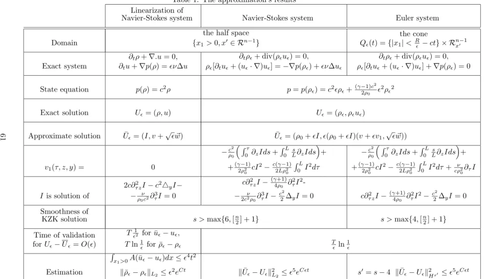
However we start the viscous case with linear problem to compare the errors for the linear and non linear problems (see table 1).
3.1
Validity of the KZK approximation for non viscous
thermoellastic media
On the one hand one considers the Euler system for ˜ρǫ(x1, x′, t), ˜uǫ(x1, x′, t):
∂tρ˜ǫ+ div(˜ρǫ˜uǫ) = 0 , ρ˜ǫ[∂tu˜ǫ+ (˜uǫ.∇)˜uǫ] = −∇p(˜ρǫ), (100)
and on the other hand a non trivial solution I of the problem
c∂2 τ zI − (γ + 1) 4ρ0 ∂2 τI2− c2 2∆yI = 0, (101) for some initial condition
I(τ, 0, y) = I0(τ, y).
The solution I as a function of (τ, z, y) is periodic in τ of period L. One constructs in this case for the KZK approximation a solution for (x1, t) positive
and negative using initial data compact in x for t = 0. The theorem 2 ensures for initial data I(τ, 0, y) ∈ Hs′
with s′ > [n 2] + 1
the existence of a solution I(τ, z, y) ∈ C(|z| < R; Hs′


![Figure 9: Wave profiles of the solution of KZK equation (39) corresponding to different δ; N = 5 (see [10, p.81]).](https://thumb-eu.123doks.com/thumbv2/123doknet/14661715.554402/69.918.208.752.386.604/figure-wave-profiles-solution-kzk-equation-corresponding-different.webp)
