A design for a high-density focused ultrasound array addressing and driving system

A Design for a High-Density Focused Ultrasound Array Addressing and

Driving System

by

R. Erich Caulfield B.S. in Physics and Mathematics,

Morehouse College, 1998

M.S. in Electrical Engineering and Computer Science Massachusetts Institute of Technology, 2001

SUBMITTED TO THE DEPARTMENT OF ELECTRICAL ENGINEERING AND COMPUTER SCIENCE IN PARTIAL FULFILLMENT OF THE REQUIREMENTS

FOR THE DEGREE OF

DOCTOR OF PHILOSOPHY IN ELECTRICAL ENGINEERING AND COMPUTER SCIENCE

AT THE

MASSACHUSETTS INSTITUTE OF TECHNOLOGY ... September 2005 ._

L FE'

ds i

02005 Massachusetts Institute of Technology All rights reserved

_ / Signature of Author: Certified by:. MASSACHUSETT-S INSTITUTrE OF TECHNOLOGY JUL 1 2006 LIBRARIES

Department of ElectricatEngineering and Computer ScienceARCHVEs September 28, 2005

<( x~~~~n

77 JCKullervo Hynynen

Professor of Radiology, Harvard Medical School Thesis Supervisor

Certified by i ; N

James7 oberge

//

.> <:.

Pro

orf

Eltrical Engineering

-~ ~' Arthur C. Smith Chairman, Committee on Graduate Students Department of Electrical Engineering and Computer Science

-A Design for a High-Density Focused Ultrasound -Array -Addressing and

Driving System

by

R. Erich Caulfield

Submitted to the Department of Electrical Engineering and Computer Science on September 29, 2005 in partial fulfillment of the requirements for the Degree of Doctor of

Philosophy in Electrical Engineering and Computer Science

Abstract

The feasibility of using focused ultrasound as an effective means of destroying malignant and benign tumors has been demonstrated in numerous studies. Research into methods for delivering the energy used in therapeutic applications has primarily used multi-element arrays, with phased array techniques offering the most flexibility. While these methods have proven effective in the ablation of tumors in vivo, limitations exist in several areas, which have prevented further advances from being made. In order to achieve tighter control over focal volume and increase beam steering capabilities, the number of elements used in phase array design will have to be increased. However, issues related to cost, matching, interconnects and cable assembly size have prevented high-density arrays from being realized as a practical means for treatment.

The goal of this research was to demonstrate the feasibility of designing and testing a relatively low-cost system that could effectively drive several thousand elements, while minimizing the size of the cable assembly that delivers power to the array. Use was made of flexible circuit technology as well as a novel method for addressing each channel. An investigation of a new technique for phase assignment in phased array configurations was also conducted to determine an optimal balance between the number of input lines and the quality of beam steering and focus control.

Thesis Supervisor: Kullervo Hynynen Ph.D.

Title: Professor of Radiology, Harvard Medical School, Brigham and Women's Hospital Thesis Supervisor: James Roberge, Sc.D.

Acknowledgements

I would first like to thank my thesis advisor, Kullervo Hynynen, for his guidance, support, patience, and insight during my PhD research. It has been a great honor to have worked and learned under the mentorship of such an insightful, forward thinking, skilled and inspiring scientist. His consistent encouragement to reach beyond the boundaries of traditional thinking, to create new and meaningful knowledge, towards better service to humankind will, no doubt, be one of the defining influences of my time in graduate school. I would also like to thank my thesis co-advisor, James Roberge, who has been an abundant source of technical knowledge, engineering acumen, and scholarly wisdom. It has truly been a privilege to have been guided by such an accomplished teacher, thinker, and pioneer. I would also like to thank, Roger Mark, who has served on my thesis committee. His advice and encouragement has been critical in helping to navigate the doctoral program over the last two years, when careful planning and directed thought were most necessary.

I would like to thank my colleagues at the Focused Ultrasound (FUS) Laboratory at the Brigham and Women's Hospital, both past and present. The wonderfully collaborative ethos, in which everyone is always available to support one another, both professionally and personally, will be the source of many memories. I especially would like to thank Jose Juste and Sai-Chun Tang for their inexhaustible knowledge, time and help in designing and assembling my PCB's. I am also thankful for the insight, humor and kindness of Xiang-Tao (Steve) Yin, whose MATLAB code served as the foundation for much of my simulation work, and whose advice on the doctoral process has been a great help. I am grateful to Greg Clement for our many conversations on physics and his keen insights into the finer points of phased array operations. I am also indebted to Nathan McDannold for his tireless help with MATLAB and in keeping my computer operating and my data safe and accessible. I would also like to thank Danish Khatri, who has been a great source of encouragement, common sense and circuit advice. In addition, I would like to thank Susan Agabian, whose kind humor and assistance in testing and verifying a large part of my hardware has helped to make even the tedious

aspects of research enjoyable. I am also grateful to Randy King and P. Jason White for teaching me most of what I've learned about transducer design and fabrication. I am indebted to Keiko Fujiwara who never failed to acquire whatever parts or equipment I needed, in time to meet the many deadlines I faced near the end of the PhD process. I am also grateful to Sham Sokka, who first invited me to come and visit the FUS lab, and who encouraged me to think about joining. I will forever be grateful for having the chance to work with Vince Collucci, Christopher Conner, Thomas Gauthier, Manabu Kinoshita, Sonali Palchaudhuri, Scott Raymond, Elisabetta Sassaroli, Nickolai Sheikov, Christina Silcox, Karen Tam, Natalia Vykhodtseva, Yong-Zhi Zhang, and Lisa Treat, who have been wonderful colleagues and friends.

Outside of the FUS laboratory, I would like to thank Albert Chow for his advice on amplifier design and help in circuit simulation, M. Mekhail Anwar for his insights in analog circuit design, and Winston Timp for his help in designing the software interface for the HDAADS. I am also grateful to Rashid Kahn and Viki Patel at Imagineering Inc for their insights while fabricating the HDAADS, as well as Granger Scofield at Apex Microtechnology for his guidance in designing the input amplifier for the HDAADS. I am eternally grateful to the MIT Graduate Student Office and Dean Isaac Colbert for his mentorship since my arrival at MIT, and for the funding I have received during a significant part of my tenure in graduate school. I would also like to thank Marilyn Pierce and Peggy Carney in the EECS Graduate Office for their support and guidance over years. I will forever be thankful for having been apart of the MIT Graduate Student Council, Black Graduate Students Association and Tang Hall Residents' Association, which have been the cornerstone of my co-curricular education at MIT. I would also like to thank the MT Administration and MT Corporation for sharing with me a spectacular vision for a greater MIT.

Finally, I would like to thank my friends and family, especially my sister, Sharron, brother, Buhl, mother, Audrey, and my grandparents, Douglas and Dorthy who believed in the impossible, and who have made the improbable an inevitability. I also hold in my heart special gratitude to my nephews, Tre' and Marcus, to whom I dedicate this thesis-you have continually inspired me.

Table of Contents

1 Introduction

1.1 Background ... 13

1.2 Focused Ultrasound (FUS) Surgery ... 14

1.3 The Current State of the Art ... 17

1.4 Limiting Factors for High Density FUS Arrays . ...18

1.5 Specific Aims ... 21

1.5.1 Phase Assignment Protocol ... 22

1.5.2 Phase Assignment and Addressing Implementation ... 24

2

Phased Array Model and Simulations

2.2 Material and Methods ... 26

2.2.1 Numerical Simulations ... 26

2.2.1.1 Simulation Parameters ... 26

2.2.1.2 Focus metrics ... 28

2.2.1.3 Array Size ... 28

2.2.2 Foci Near the Transducer Array Surface ... 29

2.3 Results ... 32

2.3.1 Off Axis Distance Results ... 32

2.3.3 Apodization Results ... 42

2.4 Discussion and Conclusions ... 45

3

Quantized Input Phase Model and Simulations

3.2 Material and Methods ... 47

3.2.1 Numerical Simulations ... 47

3.2.1.1. Simulation Parameters ... 47

3.2.1.2. Array Size ... 48

3.2.2 Quantized Phase Techniques ... 48

3.2.3 Equalized Phase Representation ... 49

3.3 Results ... 50

3.3.1 Quantized Phase Results ... 50

3.3.2 Equalized Phase Representation Results ... 56

3.3.3 Size Results ... 59

3.4 Discussion and Conclusions ... 64

4

Quantized Apodization and Extreme Field Effects

4.2 Material and Methods ... 66

4.2.1. Numerical Simulations ... 66

4.2.3 Large Focal Distance Effects...69

4.2.4 Energy Distribution ... 71

4.3 Results ... 72

4.3.1 Quantized Apodization Results ... 72

4.3.2 Large Focal Distance Results ... 77

4.3.3 Energy Distribution Results ... 79

4.4 Discussion and Conclusions ... 82

5

Quantized Input Phase Hardware Implementation

5.2 Methods ... 84

5.2.1 System Design Considerations ... 84

5.2.2 Flexible Circuit Jumper ... 86

5.2.2.1 Motivationfor the Use of Flexible Circuits ... 86

5.2.2.2 Flexible Circuit Design and Assembly ... 88

5.2.2.3 Flex to Co-axial Adaptation ... 92

5.2.3 128-Chanel Phase Selection PCB ... 95

5.2.4 Input Phase Amplifier...99

6 Evaluation of the High-density Array Addressing and

6.1 Introduction ... 102

6.2 Material and Methods ... 102

6.2.1. Numerical Simulations ... 102

6.2.2 Electrical Testing ... 103

6.2.2.1 Input amplifier Testing ... 103

6.2.2.2 Flex Circuit Assembly and Transducer Array Testing ... 103

6.2.3 Acoustical Testing ... 103

6.3 Results ... 105

6.3.1 Electrical Testing Results ... 105

6.3.2 Acoustical Testing Results ... 107

6.4 Discussion and Conclusions ... 115

7

Conclusions and Recommendations for Future Research

7.2 Future Work ... 119

7.2.1 The Current Model ... 119

7.2.2 An Alternate Amplifier ... 120

7.2.3 A Single Chip Implementation ... 122

List of Figures

Figure 1.1. Diagram of a 2-element array with inter-element spacing = -4 ... 19

Figure 1.2. Diagram of a 2-element array with inter-element spacing = X/2 ... 20

Figure 1.3. Diagram of a phased array with phase assignments ... 22

Figure 2.1. Transducer Array Coordinate System ... 27

Figure 2.2 Diagram of the element contribution to the focus ... 30

Figure 2.3. Power apodization summary for a linear 128-element array ... 31

Figure 2.4. Graph of the p2 distribution along the central axis ... 32

Figure 2.5. p2 field for 128x128 element array, focus in Z = 30mm plane ... 33

Figure 2.6. p2 _{field for 128x128 element array, focus in Z = 60mm plane ... 34}

Figure 2.7. p2_{field for 128x128 element array, focus in Z = 100mm plane ... 35}

Figure 2.8. Graphs of focal distance from plane origin vs focal metrics ... 37

Figure 2.9. p2 field for 64x64 element array focus in Z=30mm plane ... 39

Figure 2.10. p2 field for 32x32 element array focus in Z=30mm plane ... 40

Figure 2.11. Graphs of array size vs focal metrics ... 41

Figure 2.12. Apodized and nonapodized p2 field and 10% contour plots ... 43

Figure 2.13: Off axis distance vs focal metrics apodized/nonapodize arrays ... 44

Figure 3.1 Graph of peak pressure squared vs number of phase increments ... 50

Figure 3.2 P 2along the central axis, infinite/quantized resolution ... 51

Figure 3.3 p2 _{field with focus in plane Z = 30mm for 4 phase increments ... 52}

Figure 3.4 p2 field with focus in plane Z = 60mm for 4 phase increments ... 53

Figure 3.5 p2 field with focus in plane Z = 100mm for 4 phase increments ... 54

Figure 3.7 Diagram of phase assignment for a 64x64 element array ... 57

Figure 3.8 Graph of phase representations for 128x128 element array ... 58

Figure 3.9 Graph of % difference between most and least represented phase ... 59

Figure 3.10 p2 field, focal plane Z = 30mm, 4 phase increments, 64x64 elements ... 60

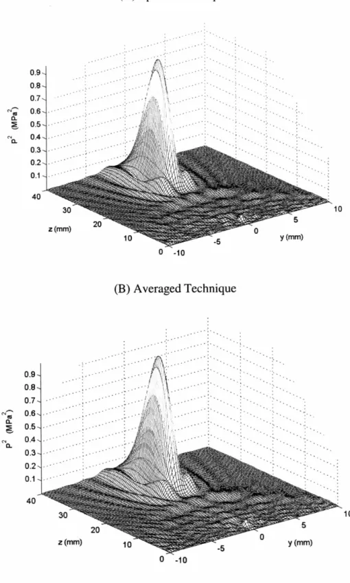
Figure 3.11 2 field, focal plane Z = 30mm, sparsed & averaged, 64x64 elements ...61

Figure 3.12 P2 _{field, focal plane Z = 30mm, 4 phase increments, 32x32 elements ... 62}

Figure 3.13 Graphs of focal metrics vs array size for infinite/quantized resolution ...63

Figure 4.1 Apodization schemes for a 128-element linear array ... 68

Figure 4.2 p2field 128x128 array, focus (0,0,100)mm, 32x32, focus (0,0,32)mm ... 70

Figure 4.3 p2field for 128x128 element array with various apodization schemes ... 73

Figure 4.4 Contour plots for 128x128 element array, various apodization schemes ... 74

Figure 4.5 Focal metrics vs off axis distance, various apodization schemes ... 75

Figure 4.6 Graphs of 1st and ₂nd peak % of the main peak ... 76

Figure 4.7 Projection of p2 128x128 array, quantized phase, focus at (0,0,100)mm...77

Figure 4.8 Graphs of grating lobe % of main lobe vs various parameters ... 78

Figure 4.9 P2 _{xy fields for Z=lmm for quantized/infinite phase resolutions ... 80}

Figure 4.10 p2 xy fields for Z=9.9mm for quantized/infinite phase resolutions ... 81

Figure 5.1 Block Diagram of High Density Array Addressing and Driving System ... 85

Figure 5.2 A block diagram of the flexible circuit interface ... 87

Figure 5.3 A diagram of the Imasonic 2725 BXXX 128-element 1.1MHz array ... 87

Figure 5.4 A diagram of the interface between a transducer array and flex circuit ... 89

Figure 5.5 A diagram of the folding process for a flexible circuit ... 91

Figure 5.7 A photograph of a flex to co-ax adapter mini PCB ... 93

Figure 5.8 A photograph of the completed flex circuit and array assembly ... 94

Figure 5.9 A block diagram of the HDAADS phase selection circuit ... 96

Figure 5.10 A photograph of the 8-channel HDAADS phase selection prototype ... 97

Figure 5.11 A photograph of the 128-channel HDAADS phase selection circuit ... 98

Figure 5.12 A schematic of the HDAADS phase input amplifier ... 99

Figure 5.13 A photograph of the HDAADS input phase amplifier PCB ... 100

Figure 5.14 A photograph of the overall HDAADS ... 101

Figure 6.1 The 128-element transducer array acoustical testing arrangement ... 105

Figure 6.2 The frequency response of the HDAADS Input Amplifier ... 105

Figure 6.3 Graph of the impedance of the 128-element array assembly ... 106

Figure 6.4 The normalized p2 field, 128-element linear array, focus (0,0,40)mm ... 107

Figure 6.5 Simulated p2 field for a 128-element linear array, focus (0,0,40)mm ... 108

Figure 6.6 Contour plots, 128-element linear array, focus at (0,0,40)mm ... 109

Figure 6.7 The normalized P2 field, 128-element linear array, focus (0,16,40)mm...110

Figure 6.8 Simulated p2 field for a 128-element linear array, focus (0,16,40)mm ... 111

Figure 6.9 Contour plots for the 128-element linear array with focus (0,16,40)mm... 112

Figure 6.10 Graph of the central axis plots for the 128-element linear array ... 113

Figure 6.11 Graph of normalized output vs input voltage for the HDAADS ... 113

Figure 6.12 Schematic of improved op am compensation ... 117

Figure 7.1 A schematic of a cable and flex circuit assembly model ... 119

Figure 7.2 A schematic of a circuit for countering cable capacitance ... 120

List of Tables

Table 3.1 Phase assignment window for 4 phase protocol ... 48 Table 7.1 Delays associated with 1 channel of the HDAADS ... 113

1 Introduction

1.1 Background

One of the primary pillars of the medical profession is to do no harm to the patient who is seeking care. Unfortunately, due to the nature of disease, which is often manifested inside the body, the physician is many times forced to make the difficult decision to cause damage on a small scale in order to achieve a greater good for the patient's overall health. This is the basic principle underlying all surgical procedures and many drugs, as incisions and medications, by their very nature, alter the body's normal functions or structure. In the best cases, the damage caused by surgery is minimal compared with the harm done by the disease. However, in the worst cases, while curing or enabling the patient to live with her or his condition, the related complications can be severely debilitating, and greatly impact the person's quality of life.

Better treatment regimens are those that only combat the disease itself or areas of the body directly affected by the illness. There are a number of non-invasive or minimally invasive methods for destroying unwanted tissue, among them lasers, devices that transmit microwave or radiofrequency EM waves, and focused ultrasound (Adams et al. 1996;Algan et al. 2000;Amichetti et al. 1991;Arefiev et al. 1998;Arustamov, Mukhtarov, & Arustamov 2000;Bagshaw et al. 1991;Burak, Jr. et al. 2003;Cioni et al. 2001;Clement, Connor, & Hynynen 2001;Gelet et al. 2000;Goffinet et al. 1990;Hacker et al. 2004;Hoffman et al. 2002;Hynynen & McDannold 2004;Jolesz et al. 2004;Koehrman et al. 2000;Melliza & Woodall 2000;Phipps et al. 1990;Prior et al. 1991;Sato et al. 1998;Sherar et al. 2001;Viguier et al. 1993;Watanabe et al. 1995). These procedures, which offer an alternative to traditional surgery, primarily work using thermally induced tissue destruction resulting from protein denaturation or coagulation. Since these instruments can deposit energy in a highly localized manner, the effects on surrounding tissue are minimized, thus reducing ancillary damage. However, in most cases, there are limitations that have prevented them from gaining greater use as substitutes for surgical treatment.

Lasers, because they are, in essence, light sources can only be used topically, as energy is absorbed directly at the surface of the skin. Even when attached to a probe, they still require an incision or other opening to be used internally. Thus, their utility in treating areas inside of the body is limited. Microwave or RF devices also offer an option for non-invasive treatment. While they are able to deliver energy into soft tissue, they too are limited to volumes near the skin's surface. One method which offers greater promise for non-invasively treating deeper tissue volumes without damage to surrounding areas is focused ultrasound (FUS).

1.2 Focused Ultrasound (FUS) Surgery

The use of ultrasound (0.5 to 10MHz) for therapeutic applications has been studied extensively over the last several decades, for a number of uses including tumor destruction (Chen et al. 1993;Chen et al. 1999;Prat et al. 1995;Rowland et al. 1997;Sibille et al. 1993;ter Haar et al. 1991;Vaezy et al. 2000;Yang et al. 1992;Yang et al. 1991;Yang et al. 1993), drug delivery (Unger et al. 1998), gene therapy (Greenleaf et al. 1998;Kim et al. 1996;Madio et al. 1998;Miller et al. 1999;Unger, McCreery, & Sweitzer 1997), thrombolysis (Francis & Suchkova 2001;Porter et al. 1996), damage via cavitation (Miller et al. 2000;Prat et al. 1994;Vykhodtseva, Hynynen, & Damianou 1994), blood vessel occlusion (Delon-Martin et al. 1995;Hynynen et al. 1996b;Rivens et al. 1999), and selective opening of the blood brain barrier (Hynynen et al. 2001a;Vykhodtseva, Hynynen, & Damianou 1994). As early as 1927, ultrasound has been investigated as a treatment option for cancer and other diseases (Nakahara & Kabayashi 1934;Szent-Gorgyi 1933;Wood & Loomis 1927). Research has shown that ultrasound can be used to treat a number of different areas of the body including: the eye (Coleman et al. 1985), prostate (Bihrle et al. 1994;Chapelon et al. 1999;Foster et al. 1993;Gelet et al. 1999;Madersbacher et al. 1993;Madersbacher et al. 1995;Mulligan et al. 1998;Nakamura et al. 1997;Saleh & Smith 2005;Sanghvi et al. 1996;Vallancien et al. 1992), liver (ter Haar et al. 1998;Vallancien, Harouni, Veillon, Mombet, Prapotnich, Bisset, & Bougaran 1992), kidney (ter Haar, Rivens, Moskovic, Huddart, & Visioli 1998;Vallancien, Harouni, Veillon, Mombet, Prapotnich, Bisset, & Bougaran 1992), bladder (Vallancien et

treatment affords the same benefits as traditional surgery, in that it provides an effective method for neutralizing the effects of unwanted tissue. For some difficult to reach parts of the body, ultrasound can be delivered via interstitial probes (Diederich et al. 1996;Hynynen & Davis 1993;Lafon et al. 1998), intravasular catheters (Hynynen et al. 1997;Zimmer et al. 1995), and intracavitary applicators (Foster, Bihrle, Sanghvi, Fry, & Donohue 1993;Hutchinson & Hynynen 1996;Sokka & Hynynen 2000). However, because FUS can be completely non-invasive technique, it lacks many of the drawbacks associated with common surgical procedures. For example, FUS offers treatment without bleeding or external scarring, and as a result, a decrease in recovery time and risk of infection (Hynynen 1996). Avoiding many of the complications of surgery, FUS has potential as cheaper and safer method for fighting tumors and others illnesses not currently treatable by other techniques.

While ultrasound has shown promise as an effective method for inducing cell death in pathological tissue for more than half century, for a long time its use had been limited by insufficient means for monitoring and evaluating its effects. A number of modalities have been considered for observing bio effects, among them X-rays and other imaging schemes that use ionizing radiation (Fallone, Moran, & Podgorsak 1982;Gelet, Chapelon, Bouvier, Rouviere, Lasne, Lyonnet, & Dubernard 2000;Jenne et al. 1997). However, these systems are constrained by the long-term harm that could be done to the patient. Another method is the use of thermocouples for measuring temperature elevation (Clarke & ter Haar 1997;Duck & Starritt 1994;Fried et al. 2002;Goss, Cobb, & Frizzell 1977;Lele & Parker 1982). However, this process requires implanting the devices inside of the patient, which negates many of the benefits of non-invasive treatment. The use of diagnostic ultrasound for monitoring has also been investigated (Fry 1968;Madersbacher, Pedevilla, Vingers, Susani, & Marberger 1995;Sanghvi et al. 1999;Sheljaskov et al. 1997), but its utility is restricted to soft tissue, as ultrasonic waves are obstructed by air and bone (ultrasound for therapeutic applications also suffers from this limitation, though in a less severe way, since we are only interested in how the waves travel in one direction). The imaging modality enables the effective monitoring of temperature, and has helped facilitate the rapid progress of FUS as a viable treatment option is Magnetic

Resonance Imaging (Chung et al. 1996;Cline et al. 1995;Hazle et al. 2002;Hynynen et al. 1993;Hynynen et al. 1996c;Ishihara et al. 1992;McDannold et al. 1998;Stepanow et al. 1995). Because MRI is a non-ionizing process, it can be used repeatedly without long-term harm to the patient or technician. Moreover, its ability to image a variety of different tissue types has enabled it to be used in numerous areas inside the body. With this repeatability and flexibility, MRI has helped facilitate the evolution of FUS into the

most promising non-invasive alternative to traditional surgery.

The basic principles underlying FUS involve concentrating high frequency sound waves inside the body at a designated location, called the focus, while minimizing pressure levels elsewhere. At therapeutic frequencies, waves can be made to constructively interfere at a specific location, thereby delivering a considerable amount of energy to that position. Because there is mostly destructive interference at locations outside of the focus volume, little energy is deposited there. This can be done effectively because sound has a relatively low absorption rate in soft tissue, thus enabling increased delivery only at the desired places. For example, an ultrasound wave at 1.0 MHz has a wavelength of only 1.5mm, but has a penetration depth close to 100mm (Hynynen & Lulu 1990). As a result, the possibility exists for resolution on the order of several millimeters and a treatment depth of tens of millimeters or more inside of the patient. The result is a method that can be used to safely and precisely destroy unwanted tissue without damage to healthy adjacent areas.

Investigations have centered around two major mechanisms for ablating pathological tissue using ultrasound: temperature elevation and cavitation. In the thermal regime, which is the more commonly used of the two methods, sound energy is converted directly into heat as the waves are absorbed by the tissue. This process is well-modeled and lends itself to monitoring using MRI (Damianou, Hynynen, & Xiaobing 1995;Hill et al. 1994;Lizzi & Ostromogilsky 1987) Using this method, temperature elevations of 20-30°C above ambient body temperature can easily be generated (Daum & Hynynen 1999). In the event of sufficiently high acoustic pressures, small gas bubbles can sometimes form. This process is called cavitation, and can lead to local temperature increases of

2000° K or more, as bubbles expand and violently collapse releasing tremendous amounts of energy (Apfel 1982). While cavitation has also been extensively studied, the exact location of bubble formation cannot be predicted as accurately.

1.3 The Current State of the Art

In both the thermal and cavitation regimes, two basic arrangements have been used for sonication: single-element (transducer) configurations and multi-element array designs. Single element systems offer a simple option for exploring ultrasonic effects on tissue, while multi-element arrays provide a more flexible alternative for diagnostic and therapeutic applications. Single-element devices are fashioned from a solid piece of PZT (Lead-Zirconate Titanate) or some other piezoelectric or piezocomposite material, which reversibly deforms when a voltage is applied across it. By applying a periodic voltage to a block or plate of the material while it is submerged in a liquid, sound waves are generated, which can then be used for diagnostic or therapeutic purposes. To achieve the focusing needed for treatment, the transducer itself will often be constructed so that it is curved. Based on the geometry of the element, a point in space is created where most of the waves will constructively interfere once the device is active. In many cases the focus is much smaller than the area being treated.

Because the focus is relatively tiny, in order to provide utility during treatment, it would need to be moved. However, with single phase systems the only way to move the focus is to move the transducer itself, which would require using a positioning system, which may not be possible due to the transducer's location, e.g. inside of an MRI magnet. As such, in order effectively treat larger volumes a method for easily steering the focus needed to be developed.

During the last twenty years, devices called phase array transducers have become more prominent, as they provide electronic beam steering capabilities, as well as enabling compensation for a number of factors which distort the ultrasound field (Benkeser et al. 1987;Buchanan & Hynynen 1994;Cain & Umemura 1986;Clement & Hynynen 2000;Daum & Hynynen 1999b;Diederich & Hynynen 1989;Do-Huu & Hartemann

1981;Ebbini et al. 1988;Fan & Hynynen 1995;Fjield & Hynynen 1997;Frizzell et al. 1985;Hutchinson & Hynynen 1998;Hynynen et al. 1996a;Hynynen & Jolesz 1998;Ibbini, Ebbini, & Cain 1987;Maslak 1975;McGough et al. 1994;Sokka & Hynynen 2000;Sun & Hynynen 1998). Phased array systems are multi-element configurations that vary the phases of each individual element in order to create the focus. These transducer arrays need not be of any particular geometry to be effective, as adjustment to the phase can be made to achieve various focal locations. Phased arrays also provide the ability to create multiple foci at once, whose position(s) can be moved almost instantaneously by simply varying the input signal. This feature is especially important because being able to create multiple foci has the potential of improving heating distribution (Ebbini & Cain 1989). Currently, most FUS phased array systems are 1-dimensional and employ from 5 to 200 elements, with a few 2-dimensional systems using several hundred elements (Daum & Hynynen 1999a).

1.4 Limiting Factors for High Density FUS Arrays

In order to develop systems that exhibit greater focus control, the number of elements will need to be increased. This fact results from the relationship between focal precision, beam steering, and inter-element spacing. Figure 1-1 shows a 2-element array with frequency f and inter-element spacing of - 4X. For this simple case, the waves from the two elements are in phase at the focus. However, there are numerous other places where the waves constructively interfere (called grating lobes), which present a problem for clinical uses, where significant constructive interference is to be minimized outside of the focal volume. In this example, there are only two waves that intersect at the focus. This is the same number that intersect in other places in the field. For arrays with more elements, there would be many more waves merging at the focus than at any other place in field, making it possible to deposit a large amount of energy there while imparting little elsewhere.

If the elements were to be moved farther apart the number of constructive interference points would increase. The number would also increase if the focus were to

be moved away from the center axis. In order to reduce the creation of grating lobes, the two elements would have to be moved closer together. Figure 1-2 shows a similar 2-element array, but with an inter-2-element spacing of X/2. In this configuration, there is a significant reduction in the number of constructive interference points, yielding a more cleanly defined focal region. Because there are only two elements in this illustration, there is a line of interference points along the center axis between the two elements. However, if more elements were added with the same spacing, this region would become less prominent as the pressure at the focus would dramatically increase relative to other locations in the field. It is this relative difference in pressure values that creates a useful focus, since extra-focal regions are heated much less, by the resulting lower pressures.

4 d = -4X .

Element I Element 2

-

3.= Focus

* = Other areas of constructive interference

Figure 1.1 A diagram of a 2-element array with frequency f, wavelength X and inter-element spacing of d = - 4X.

d = /2

Element I Element 2

Figure 1.2 A diagram of a 2-element array with frequency f and wavelength X and inter-element spacing of d = A/2.

As a result of the reduction in the number of grating lobes, the <X/2 spaced arrangement provides the optimum spacing for beam steering. From Figure 1-2 it can be seen that moving the focus to other locations using this inter-element distance, the possibility for creating additional constructive interference points is minimized. It might appear at first that moving the elements closer than X/2 could yield even better results. However, decreasing the spacing further would have no additional benefit as there would be no increase in focal intensity, i.e. all of the waves are already in phase at the focus, and as such, no additional pressure increases could be accomplished. In addition, from Figure 1-2 it can be seen that a further reduction in grating lobes would not result since the minimum number has already been achieved.

Having shown the advantages of moving to X/2 spacing, now consider a typical therapeutic frequency of 1.1 MHz, X = v/f = (500Om/s)/(1.1MHz) = 1.36mm and X/2 = 0.68mm, where v is the speed of sound in water and f is the frequency of the signal. With

this spacing, the individual elements would have to be relatively tiny, and in order to cover a large enough area to deliver an appreciable amount of power, there would have to be a large number of them. As such, one of the key components to increasing the capabilities of FUS systems is the ability to design and drive arrays with a large number of small elements. However, there are a number of issues that have prevented higher density arrays from being implemented in a practical manner.

One constraint is the problem of cost. Currently, many driving systems for FUS arrays rely on high Q transducers and accompanying resonant amplifiers. These high power systems are needed because a smaller number of elements requires that each individual transducer supply a significant amount of power in order for the array as whole to be useful. Because many of these configurations rely on finely tuned resonant circuits, the components needed to construct them tend to be expensive and sometimes difficult to replace. In addition, the driving circuitry has to be manually matched to the transducer load for each channel, which can often be a very time-intensive process. Another issue is that, for a given application, as the number of elements increases, the size of each element tends to decrease. As a result, it becomes increasingly difficult to form connections (interconnects) to each one. The last major limitation is the size constraints of the cabling that delivers power to the array. As the number of elements increases, the bulk of the wires going to the assembly becomes excessively large. This is especially of concern when the device is to be used inside the body.

If more effective means of developing high-density FUS systems are to be developed in the future, the issues of cost, matching, interconnects and cabling/complexity will have to addressed.

1.5 Specific Aims

This research examines a method for effectively driving an array of thousands of elements for use in therapeutic ultrasound. The first section of the study is an examination of the theory behind a novel phase assignment scheme, which allows a large

number of elements to be driven while using relatively few input lines. The second section assesses a small-scale implementation of the phase allocation process, which addresses the cost, matching, and cable assembly issues.

1.5.1 Phase Assignment Protocol

Perhaps the greatest challenge to achieving higher density phase arrays lies in the constraints of the cable assembly that delivers power to the array. Traditional designs have used a one-to-one correspondence between the driving signal wire and its corresponding element in the element in the array. Figure 1-3 illustrates the basic functioning of a phased array with five elements:

Dhi A = A *7'rr

n

L

Figure 1.3 A diagram of a phased array with phase assignments

Assuming that all of the transducers use the same frequency, in this case transducer 1 serves as the 00 phase reference for the others, meaning no adjustment is needed for it. Since the distance from transducer 2 is different from transducer 1, its phase has to be

shifted in order for it to constructively interfere with transducer l's wave at the focus. The adjustment is based on the simple geometry of the triangle formed between the two elements and the focus. Here, the difference is X/4, which when converted to a delay for a sinusoid, becomes (27/X)*X/4 = n/2 radians or 90°. In a similar fashion, the phase of transducer 3 can be adjusted so that it is in phase with the others at the focus. This same process is performed for each of the transducers in the array. To move the focus, one only need follow the same method described, adjusting the phases of each element accordingly. This technique also allows for the creation of multiple foci by using combinations of elements.

It should be noted that as the number of elements grows, so does the number of phase assignments and wires. The problem is further compounded by the need to shield the wires to minimize electrical interference. This is usually done by making use of coaxial wires, whose price has been found to scale inversely with the size of the wire. Because high-density arrays will require very small wires, which may not be obtainable,

their cost and availability prohibit use in large numbers. Thus, it would be very difficult, using existing methods, to design practical arrays that could have four or five thousand elements.

The solution which this study examines is to quantize the phases available at the input of array. A variation of this concept was explored by Fjield et al in 1999 in the context of low-profile lens and showed promise for use in other areas (Fjield, Silcox, & Hynynen 1999). The central idea is that instead of allowing practically infinite phase resolution for creating the focus, only a relatively small number of phases will be used. All of the phases that lie within a specified window are assigned to a single phase at the center of the range. For example an element whose required phase falls between 45 to 135° would be assigned a phase of 90°. Done this way, the need for each individual element to have its own phase and unique wire to deliver it is eliminated. By having each element share input lines with others requiring similar phases there is a tremendous reduction in the number of discrete wires coming into the system. For example, an array with 10000 elements, and only 4 different phase increments: 90°, 180°, 270°, and 360°,

could be managed by only 34 lines (4 input signal lines and 30 control lines). It should be noted that the number of input wires required does not increase as additional elements are added, thus amplifying the benefit as the number of channels grows.

MATLAB simulations, making use of the Rayleigh-Sommerfeld sum and Huygens Principle (where individual elements are treated as being made of smaller simple sources whose contributions are summed to give the field for that particular element) were developed in our laboratory, which describe focused ultrasound propagation in a homogeneous medium. The program can be varied along one or more parameters, including: the number of elements, their center-to-center spacing, the wavelength of the sound and propagation medium. Beam steering capabilities for arrays ranging in size from 64x64 to 128x128 elements were examined, with foci located from 20 to 60mm from the array surface, and from 0 to 30mm from the center of the plane parallel to the array. The frequency used in the simulations was 1. 1MHz and the medium was water. A number of metrics were used to describe the quality of the focus, including: 3dB length and volume, side lobe to main lobe ratio, and peak intensity.

1.5.2 Phase Assignment and Addressing Implementation

The development of large scale, high-density focused ultrasound driving systems has been primarily hampered by cost and a lack of technology capable of rendering them feasible. Traditional driving systems have relied on high Q ceramic transducers and tuned amplifiers to deliver ultrasound. However, these systems are expensive and require a significant investment in time to make them operational. In conjunction with recent advances in transducer technology and in response to the constraints imposed by traditional systems, our laboratory has conducted research into improving how ultrasound is created and controlled.

One area where progress has been made is in developing relatively new broadband piezocomposite materials, which have allowed us to operate over a wide range of frequencies. Our laboratory has developed a system that can deliver 1-2 W of

2000+ channels (Sokka 2003). This configuration significantly improves the ability to effectively delivery ultrasound and solves many of the problems associated with resonant transducers and their accompanying amplifiers. However, while this configuration does offer the ability to effectively drive a relatively large number of channels, it remains limited by its one element to one driving wire power delivery scheme. This restriction makes it somewhat difficult to make full use the system's scaling capabilities.

In order to overcome the limitations of current designs and also to verify simulation results, a 128 channel addressing and driving printed circuit board (PCB) was designed, built, and evaluated. The board provides 0.5 to 1.7 W of electrical power per channel, is broadband from DC to 5 MHz and is scalable from 128 to 10000 or more channels. This design requires only 24 input lines for its 128 channels and has a channel per unit area 2.5 times that of the previous broadband system. The board was used to drive a 128-element piezocomposite transducer array that was developed in our laboratory. The PCB was connected to the array via a novel flexible circuited designed to mate with connecting pad on the back of the transducer case. The pressure field was measured in water, while operating at 1.1 MIHz. Experimental results were compared to simulations to access functionality. The system offers one implementation of the quantized phase concept, and provides proof that a relatively low-cost high-density array driving circuit could be fabricated using existing technology.

2

Phased Array Model and Simulations

2.1 Introduction

In this chapter we examine the focal quality and beam steering capability of planar phased arrays. There are a number of issues related to phased arrays that require methods for mitigating their effects, among them the appearance of grating lobes (de Jong et al. 1985) and other unwanted areas of constructive interference, which occur near the transducer surface. To assess the benefits and limitations of using this configuration for treatment applications, a computer model was developed, that would provide insight into the impact of various physical parameters on the ultrasonic field. Among the factors considered were array size and power distribution. It was discovered that for larger aperture arrays, when the focus was placed near the transducer surface, apodization of the element power was required to offset undesired pressure increases between the focus and array. The relative effectiveness of this weighing technique for reducing the prominence of these unwanted areas was investigated. The aim of the section is to lay a foundation upon which further work can be done towards practical implementation of high-density array systems.

2.2 Material and Methods

2.2.1. Numerical Simulations

2.2.1.1. Simulation Parameters

The pressure fields were simulated using the Rayleigh-Sommerfeld sum:

p(x,y,z)= -

d exp j(

-

)-dia

(2.1)

i=l cA d A

Here p = pressure (Pa), P = total acoustic output power of the array (W), p = density of the medium (kg m'3), c = speed of sound in the medium (m/s), A= total surface area of the array (m2

), f = resonant frequency of the array (frequency at which the array has its largest output for a given input signal), S = area of corresponding element (m2), a = the attenuation coefficient (Np/m/MHz), d = distance from the field point to the

corresponding element (m), = the phase of the source, and i = the corresponding element index,. For this study each element was modeled as being composed of 9 simple sources that all used the same phase. The resulting pressure field was found by using Huygen's Principle, which states that the field at a given point is the superposition of the contributions from all of the active elements, in this case, simple sources in an array. Simulations were run for a 128x128, 1.1 MHz, array with 0.44mm x 0.44mm elements having center-to-center diagonal spacings of 0.64mm and x and y spacings of 0.45mm. It should be noted that the X/2 is equal to 0.68mm, and that the diagonal distance was constrained by this value, since it is the farthest distance between adjacent elements, and guarantees that elements along all dimensions satisfy the X/2 requirement. The medium was assumed to be water, where the speed of sound, c = 1500m/s, the density, p = 1000kg/m3_{and the attenuation coefficients, a = 2.88x10-}4_{Np/m/MHz (Duck 1990). The}

total output power of the array was 1W. The transducer orientation can be seen in Figure 2.1: Focus at (30,30,30) X

¥

Figure 2.1 Transducer Array Coordinate System I F

2.2.1.2. Focus metrics

For all simulations the transducer array was located in the plane Z = 0mm, with its center at the origin, and sound propagating the positive Z direction. The resolution in the calculated pressure field in the x, y, and z directions was 0.22 mm, yielding a volume resolution of 1.lx10- 2 mm3. This was chosen to give sufficient information about the field structure, while minimizing the simulation time. For each case, the focus was electronically steered to multiple locations to determine the effect on peak focal intensity, the ratio of side lobe to main lobe, the 3dB length, x and y width and volume, and the overall intensity field. The side lobe ratio and 3dB length and widths were measured by visual inspections of the associated graphs and the peak pressure squared and 3dB volume were calculated by the program. The focus location ranged from X = -30mm to +30,Y = -30mm to +30 and Z=Omm to 100mm. Unless otherwise noted, when the focus was steered to a position away from the origin of given Z-plane, it is done so in X=Y increments of 10mm, e.g. for the plane Z=30 the focus would be steered to (0,0,30), (10,10,30), (20,20,30) and (30,30,30). This method was chosen as it reveals the effects of the asymmetry of the square planar array. The upper bound of 30mm for x and y was selected because it is approximately equal to 28.8mm, which is the distance from the center to the side edge of the array, and consequently of the converging region of the field. All simulations were written using MATLAB and were run using a PC with an Athlon XP 2800 processor.

2.2.1.3. Array Size

To investigate the effects of array size on focal control, the dimensions of the 2D array were varied. In each scenario described in section 2.2.1.2, the array size was increased from 32x32 to 128x128 elements with simultaneous x and y steps of 16 elements (an aperture increase of 7.2mm). The impact was measured using the same metrics examined in section 2.2.1.2. In this case the focus was steered in the plane Z=30mm at (0,0,30) and (10,10,30). These locations were chosen as they represent a useful sonication depth, and lie with the array field (edge of the array) of most sizes considered.

2.2.2 Foci Near the Transducer Array Surface

One of the features of planar phased arrays is the appearance of a continuous pressure "ridge" leading from the focus to the surface of the transducer, when the focus is brought close to the array. This phenomenon does not occur with spherical transducers and results from the fact that, in terms of area, planar transducers do not map directly to their curved counterparts. Recall that in traditional non phased array transducers the focus is geometrically created by constructing the transducer in such a way that all points on the surface are equidistant from the desired focal location. As such, when the array is excited, all of the resulting waves are all in phase at the focus. Planar phased arrays attempt to mimic this kind of behavior by adjusting the phases of each element so that the waves constructively interfere at the focus. This is a reasonable approximation for foci that are relatively far from the array, since for distant foci the required radius of curvature compels the array to be relatively shallow. However, the approximation breaks down nearer to the surface. Examination of figure 2.2 shows why this is the case.

In figure 2.2A, the focus is located far from the array. As such, the curved transducer and the planar transducer have approximately the same active surface area.. Of more importance is the fact that the region on the outside ring or edge of the spherical array and the elements in the outer portion of the planar array, occupy and area of similar size. However, when the focus is moved closer, as in Figure 2.2B, the difference between then two areas becomes significant. Consequently, the outer elements in the planar array will contribute much more to the focus than the corresponding section of the curved transducer. Since the waves from the elements will be converging such that their normal vectors are almost parallel. What results is large area where constructive interference will occur, thus producing the "ridge".

In order to mitigate the impact of this effect, the contribution of the outer elements has to be reduced. This is done by simply reducing the power to those elements. Since the effect is primarily distance related, the scaling should be proportional to the distance from a given element to the focus. However, recall from the Rayleigh-Sommerfeld sum:

p(xy,z)= = cA expj(- - di

i=1 d

~

~

~

~

that the pressure is also exponentially related to distance via a, the attenuation coefficient. As such the adjustment should also reflect this factor. The resulting scaling coefficient thus becomes

(2.2)

Where d, i and a have the same meaning presented in equation 2.1.

Phased Ar Transduce Equivalent C Transducer Focus I Edge Contibuton Center Conrbon Phased Array Transducer Equivalent Curved Transducer (B) -ocus I Edge ContributiMon [] Center Contribution

Figure 2.2 A diagram of the element contribution to the focus for a linear 128 element array and a spherical single phase transducer that would create the same focus. (A) Case where the focus is far from the array (B) Case where the focus is near the array

This amplitude adjustment, or apodization, is shown for a linear 128-element array with focus at (O,O,10O)mm in Figure 2.3.

(A) Nonapodized 20 40 120 20 40 60 80 1 O0 !20 (B) Apodized 20 40 60 80 100 120 Element #

Figure 2.3 Power apodization summary for a linear 128-element array with focus at (0,0,10) (A) Nonapodized, equal power case (B) 1/d exp(cxd) apodization case

While this technique has been used in diagnostic applications for increased control over grating lobes (Eaton, Melen, & Meindl 1980;Karrer et al. 1980b), it has not seen use for very near field therapeutic applications. By enabling the focus to be brought closer to the transducer surface, the flexibility of phase array technology is further enhanced.

0.02 0.015 0.01 0.005 0

{

2.3 Results

2.3.1 Off Axis Distance Results

Figure 2.4 shows the pressure squared field along the central axis (O,O,Z). for a 128x128 element array.

Central Line p2 Profile

CN CL d-S~~~~~~~~~~~~~~~~ 8 7-6 5 4 3 2 20 40 60 80 100 120 Z (mm)

Figure 2.4 A graph of the p2 distribution along the central axis (O,O,Z) for foci from Z=1Omm to 100mm in 10mm increments, for a 128x128 element array.

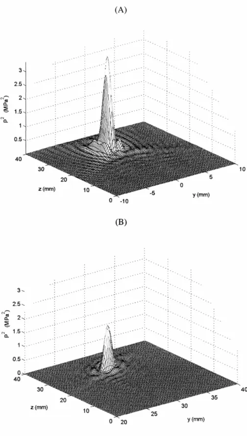
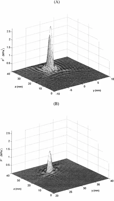
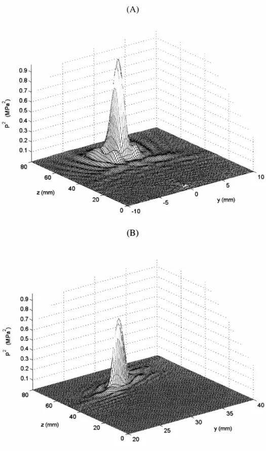
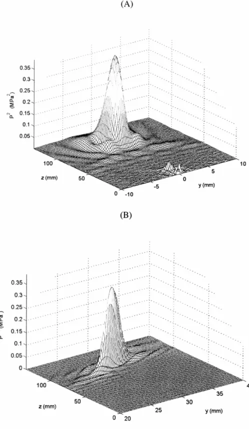
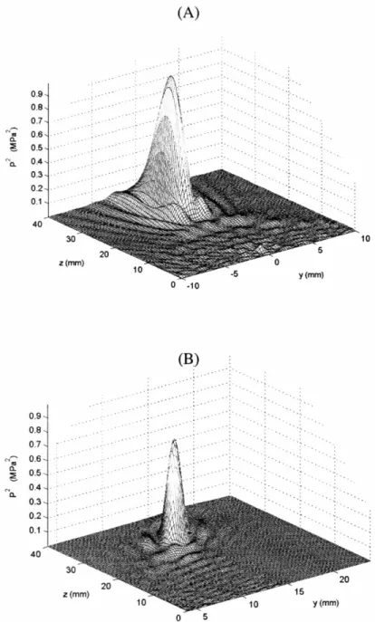
Note that the peak p2for each focus appears to decay exponentially at the focus moves away from the transducer. Also, observe that the beam length increases substantially as the focus is steered Figures 2.5-2.7 show the pressure field squared for foci at locations from Z=30mm to Z=10Omm, both at the origin and extremes (30,30,Z) of each plane.

3 2.5 ~2 a.. 6 1.5 N a.. 0.5 40 a -10 (B) .' .' . .. .' . 10 .-N~ 2~,."""'" 6 0.5--.: ... a : 40 z(mm) a 20 y (mm) 40

Figure 2.5 A diagram of the pressure field squared for a 128x128 element array (A) Focus at (0,0,30) (B) Focus at (30,30,30)

(A) 1.2 0.8 N'; a. 6 0.6 N a. _0.4 0.2 80 10 o -10 (B) 1.2 .... 1 .... .'. . . .. '"7'\ N'; 0.8

!~

Figure 2.6 A diagram of the pressure field squared for a 128x 128 element array (A) Focus at (0,0,60) (B) Focus at (30,30,60)

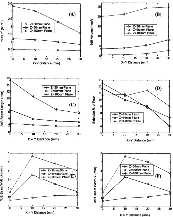
0.4 ,.... _0.3 "'1\'1 a.. 6 '"a.. 0.2 . ~. - .0" • 'f: _.' ' • . . . . . I .\\: . . rf'(~:':"" .

... ... y.i\,!\.\

Figure 2.7 A diagram of the pressure field squared (A) Focus at (0,0,100) (B) Focus at (30,30,100)

Note that in each case the grating lobes are suppressed in the field near the transducer plane at z = 0mm.

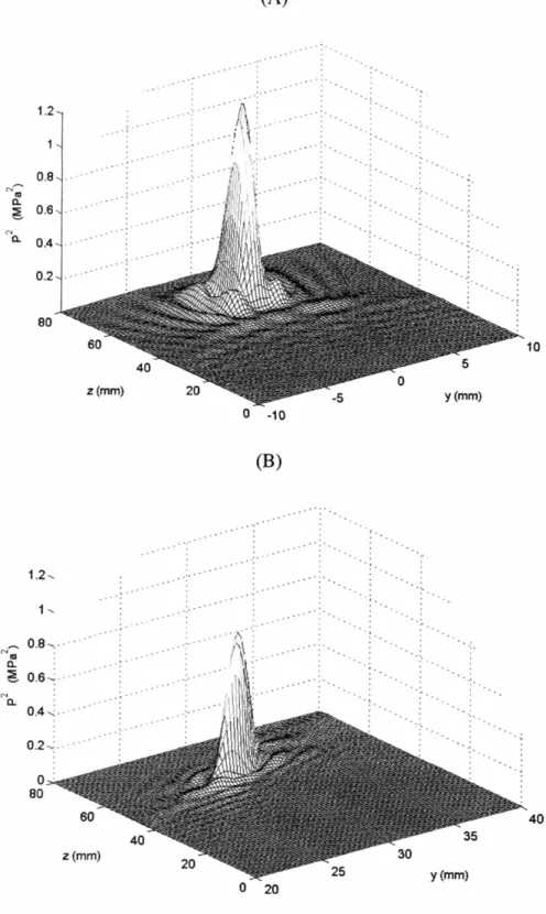
Measurements of 3dB beam length, width and volume as well as the peak pressure squared were done as a function of the x = y = n distance from the center of the plane being considered (where n=0,10,20, and 30mm). Investigation of the ratio of the largest side lobe to the main lode was also done for the same locations. The results for the planes Z = 30mm, 60mm, and 100mm are summarized in Figures 2.8. Examination of Figures 2.8A and 2.5B shows that for the plane Z = 30mm, the peak pressure squared decreases by approximately 53% as the focus moves from the origin to the x = y = 30mm corner of the plane, with the 3dB volume increasing by 430%. Also of note is the fact that for the distances farther away, the change in peak pressure is very much less. As can be seen from Figure 2.5-2.7 and Figures 2.8C and 2.8D, the 3dB beam length shortens and in general, the sidelobes decrease relative to the main peak as the focus is moved off axis. Additionally, the similarity between the x and y 3dB widths in Figures 2.8 E and F should be observed.

X=Y Distance (mm) X = Y Distance (mm) 20 E E G) E 0 co) 15 10 O0 5 10 15 20 X=Y Distance (mm) E Cu a. 0. 0 a) -r en 4o :0_(I) E A E at W a 0 25 30 X=Y Distance (mm) X = Y Distance (mm) X = Y Distance (mm)

Figure 2.8 Graphs of the relationship focal distance from plane origin and focal metrics. (A) between location and peak focal pressure squared, (B) between location and 3dB volume, (C) between location and 3dB beam length (D) between location and side lobe % of the peak pressure squared, (E) between location and 3dB X beam width, and (F) between location and 3dB Y beam width

____~

~~

(B)

2.3.2 Array Size Results

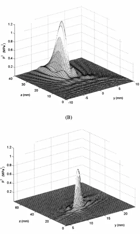
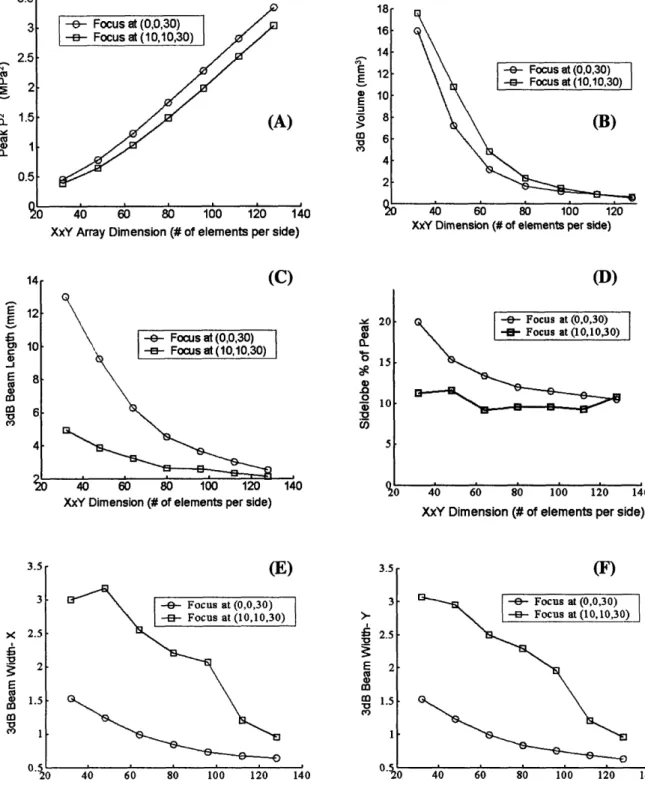
To investigate the effects of array size on the metrics discussed in section 2.3.1, the array size was varied from 32x32 elements to 128x128 elements, in increments of 16x16 elements (7.2mm aperture increase), with the same parameters and orientation described in section 2.2.2. Figures 2.9 and 2.10 show the pressure square fields for at 64x64 element array and a 32x32 element, each with 0.45mm x and y spacings, and conditions previously described for the 128x128-element array. Note that for the off axis plots, value of 14mm and 7mm were used for the 64x64-element array and the 32x32 element array respectively. These values were chosen as they lie on the edge of the array field for their corresponding transducers. Observe that there is increased grating lobe formation as the array becomes smaller, with significant extra focal constructive interference in the 32x32-element configuration.

Figure 2.11 shows the relationships between array size, the peak focal pressure squared, sidelobe to main lobe ratio, and 3dB volume, length and x and y width for focii at (0,0,30) and (10,10,30). As shown in Figures A-D, E and F, the focus, in general becomes tighter as more elements are added.

1.2 0.8 "'lIS a. 6 0.6 "'a. 0.4 0.2 40 z(mm) ... ---"'l10: .-_.- -'. .. ' ifA ' . . . . I \~.' . ..'../

\\

Figure 2.9 A diagram of the pressure field squared for a 64x64 element array (A) Focus at (0,0,30) (B) Focus at (14,14,30)

.. 0.4 0.3 .' N III a. 5 0.2 N ,. a. 0.1 (A) ...._. . o -10 (B) 10 0.4 0.3 N'; a. 5 0.2 No. 0.1

Figure 2.10 A diagram of the pressure field squared for a 32x32 element (A) Focus at (0,0,30) (B) Focus at (7,7,30)

E E a E "5 A) '20 40 60 80 100 120 140 XxY Array Dimension (# of elements per side)

-- Focus at (0,0,30)

-- Focus at (10,10,30)

(B)

XxY Dimension (# of elements per side)

Id"i'

-eo Focus at (0,0,30) -a- Focus at(10,10,30)

XxY Dimension (# of elements per side)

v 0 ti 0) .0 c0 -o._) 20 15 10 S (D) I 20 40 60 80 100 120 140

XxY Dimension (# of elements per side)

(E) .

3

)Ii

40 60 80 100 120

XxY Dimension (# of elements per side)

S >-E 'o co_'a 0) 2.5 2 1.5 . 140 40 60 80 100 120

XxY Dimension (# of elements per side)

Figure 2.11 Graphs of the relationship between array size and focal metrics. (A) between size and peak focal pressure squared, (B) between size and 3dB volume, (C) between size and 3dB beam length (D) between size and side lobe % of the peak pressure squared, (E) between size and 3dB X beam width, and (F) between size and 3dB Y beam width

3 2.5 2 (U o av 0-K (. a) 1.5 I 0.5

i

'a-_ga,

2.3.3 Apodization Results

Using the same metrics and orientation as those in sections 2.2.1 and 2.2.2, a study of the effects of varying the power used by each element was investigated for a 128x128 element array, with foci at (0,0,10) and (0,0,30). Figure 2.12 shows the pressure squared field and 10% contour plots for the 128x128 element array. Figure 2.13 shows the focal metrics for the apodized and nonapodized cases for foci in the planes Z=Omm and Z=30mm. Of note is the general closer agreement between the values in the plane Z=30mm than those in Z=0lmm, as shown in figures 2.13 A, C ,D, and E. Also, observe that the largest variations usually occur at the extremes, x=y=30mm in each plane.

(A) Nonapodized (Infinite ~hase Re~) 20 z[mm] 5 o 8 ; , , , .. .... .. .. ~~~: Apo",,,, " ~ ' •..• \. : ;\ : : . 1.:~. : N a. 2 N'; 6 a. 6 4 Beam Contour 15 14 13 12 9 10 11 z[mm] 8 7 6 1 : : : E.:.:.:- ? : : : . . ._. ._. ._. ._. ._. ._{. .}. ._. . . . . . ._.. .. ... -1 5 0.5 -0.5 : : ~ : . . . . . . . . . . . . 20 Beam Contour ..._{. . . . . . . .} -_. . 1 . 0.5 E .sO >--0.5 ..1 : : : : : : : : . 5 6 7 8 9 10 11 12 13 14 15 z[mm]

Figure 2.12 A diagram of the pressure field squared and 10% contour plots for a 128xl28 element array with the focus at (0,0,10) (A) The nonapodized case (B) The apodized case

E E E m X5 co CED 0 5 10 15 20 25 30

X=Y Distance (mm) X=Y Distance (mm)

E E =S m_E "o m₀

X

X

=

Y

=

Distance

Y

Distance

(mm)

(mm)

Figure 2.13 Graphs of the relationship focal distance from plane origin and focal metrics for an apodized and nonapodize 128x128-element array. (A) location and peak focal pressure squared, (B) location and 3dB volume, (C) location and 3dB beam length (D) location and 3dB X beam width, and (E) location and 3dB Y beam width

Cu a) E-g.. ._1 S_Ea) C m C) 83 Cv) co co

2.4

Discussion and Conclusions

Examination of Figure 2.8B shows an increase in 3dB focal volume as function of off-axis distance. It should be noted that while the 350% increase may initially seem large, at the edge of the field, the total volume is still less than 2.6mm3_{. In addition focal}

volume for the planes Z=60m and Z=lOO1mm remain relatively flat, as does the peak pressure squared, suggesting that father away from the array beam steering has less of an effect on the quality of the focus. Investigation of Figures 2.5-2.7 show the expected effects of steering, as the focus rotates towards a diagonal orientation as the beam moves to the edge of the array. However, the usual severe spreading found at the extremes of the plane are not as apparent. This is the result of the large number of elements, which help maintain the integrity of the focus, despite its location near the periphery of the array field. These results suggest that a high degree of focal precision could be maintained even when the focus is steered to the edge of field, provided that there is a sufficiently large number of elements.

Figure 2.11 shows the relationship between focal metrics and the number of elements as it relates to array size. Examination of the graph reveals the peak pressure squared and the 3dB volume are similar for both foci as function of size, implying that the localized delivery of the power is similarly effective. However, inspection of Figures 2.11 C, E, and F show that a divergence occurs between the 3dB length and width as the array gets smaller, with the length growing when the focus is at the origin, and the width when it is off axis. This is consistent with one would expect. Figure 2.11 shows that the beam steering capability begins to quickly degrade once the array becomes smaller than 64x64 elements, with the volumes of the foci both on and off axis increasing substantially below that size. This dramatic change is not surprising as the ratio of the number of elements between each successive increment begins to grow substantially at the point, e.g going from 64x64 elements to 48x48 represents a decrease of 45%, where as the reduction from 128x128 to 112x112 is only 23%. However, as Figure 2.9 shows, for a 64x64 element array, the grating lobes remain suppressed, while the sidelobes are below 15%, which is an acceptable limit. This implies that even with a reduced number of the elements, a 64x64 element device would still demonstrate good steering capability. These

results taken together with the previous outcomes for the 128x128 element array suggest that at distances where the f number (ratio between the distance from the array center to the focus and the width of the array) is between /2 and 1, phased arrays provide a useful means for effectively delivering directed power to a specific location.

Figure 2.12A shows the presence of a pressure "ridge" which occurs when the focus is brought close to the surface of a large aperture array. Figure 2.12B shows that when the power is apodized, the ridge can be reduced, though not eliminated completely. Inspection of Figure 2.13 A reveals the additional value of using this power scheme. The figure shows that for all focal positions in the Z=10mm plane, the apodized peak pressure squared is higher than that for the nonapodized case, by more than 31%in most cases. The 3dB beam length and width also show slight improvements for the nearer plane. As one might expect, the metrics for the two cases show more agreement in the Z=30 plane, where the relative differences in distance from the focus to individual elements is less. As such, apodizing the power appears to be effective for increasing array performance in the region close to the array surface, offering little benefit father away. It should be noted that, while the "ridge" is relatively small compared to main lobe, minimizing its impact is

still useful, e.g. in a situation where cavitation is occurring and thresholds for creating tissue damage have been reduced.