Design of a Flexible Containment System for
Deep Ocean Oil Spills
by
Natasha Maas
Submitted to the Department of Civil and Environmental Engineering
in partial fulfillment of the requirements for the degree of
Master of Science in Civil and Environmental Engineering
at the
MASSACHUSETTS INSTITUTE OF TECHNOLOGY
June 2013
A.RCHgVEg
FMASSACHUSE-1- INST. E OF TECHNOLOGYJUL
0 3
2013
L BRARIES
@
Massachusetts Institute of Technology 2013. All rights reserved.
Author ...
...
Department of Civil and Environmental Engineering
May 10, 2013
Certified by....
Senior Lecturer and Senior Research Engineer of
Dr. E. Eric Adams
Civil and Environmental Engineering
Thesis Supervisor
A ccepted by ... , ., ... ... . . . . .
Prof. Heidi
.tef
Chair, Departmental Committee for Graduate Students
Design of a Flexible Containment System for
Deep Ocean Oil Spills
by
Natasha Maas
Submitted to the Department of Civil and Environmental Engineering on May 10, 2013, in partial fulfillment of the
requirements for the degree of
Master of Science in Civil and Environmental Engineering
Abstract
BP needed almost 3 months to cap the Deepwater Horizon spill; improved response techniques are needed for the future. This work presents the design and deployment plan for a new type of containment system that captures the vast majority of hydrocarbons exiting the wellhead. The structure is lightweight, flexible and modular, using a passively induced chimney affect as its working principle. It is modular to create one design that fits any number and size of wells. Modularity comes from 100m sections of thin Kevlar fabric, forming a cylinder that starts several meters above the seabed and ends several meters below the sea surface. The
system is stored onshore mostly assembled until needed.
The 3m-diameter shroud induces a flow that dilutes the gas to avoid hydrate formation. Yet the velocity is sufficiently small for gas to dissolve, reducing surface gas concentrations below workers' safety thresholds. The chimney effect causes a pressure differential over the material; reinforcement ribs are required to keep the system from collapsing inward. At the shroud top, the jet enters a containment pen, which is loosely attached to the shroud allowing it to ride the waves in heave, but constraining roll, pitch and yaw. The pen diameter allows oil to separate from the water; a skimmer weir in the pen collects almost pure oil and pumps it to a tanker. An air can at the shroud top provides pre-tension that restrains lateral deflections due to a uniform current, and helps reduce the collapse due to the pressure differential. The deflection and collapse are calculated for a uniform current using catenary equations. The results are used to verify the applicability of OrcaFlex, software commonly used by the off-shore industry, which is then used to confirm the systems ability to satisfy design requirements under realistic conditions (a sea spectrum and non-uniform current).
The 'one design fits all' objective is tested by initially designing the system for a moderate size reference well, and then scaling it up (with minor modifications) to fit the Macondo well. The results confirm that one design of the system can contain spills of moderate size in
addition to those similar to the Deepwater Horizon.
Thesis Supervisor: Dr. E. Eric Adams
Acknowledgments
I would like to thank my adviser, Eric Adams, firstly for offering me this project upon my
arrival to MIT and for his endless support since. His enthusiasm and guidance have made the last two years a great learning opportunity and an incredible personal development expe-rience. I would also like to thank ENI S.p.A for making it possible for Eric and me to work on this project. Special thanks to Roberto Ferrario who was a wonderful resource on ENI's side and was a great support throughout the project. Similarly, I would like to thank Marco Calza for spending hours helping me setup the OrcaFlex model during my visit to Milan, as well as Nicola De Blasio, Mario Marchionna and Mario Chiaramonte for their support for this project. The collaboration with all of you at ENI was wonderful and I have learned a lot from
you.
At MIT I would further like to thank professor Ole Madsen for being a great teacher and help for my research. From the Ocean Engineering department I would like to thank profes-sor Thomaz Wierzbicki and his student Kirki Korfiani, profesprofes-sor Paul Sclavonous as well as professor Micheal Triantafyllou and his student Haining Zheng for making time to help me on topics that were new to me, even though I was not their student or colleague. Without all of your help my project could not have been as multidisciplinary as it has turned out to be.
I would also like to thank the other students in my lab group; Marianna, Ruo-Qian and
Godine. You welcomed me into the group in my first semester here and were a great support then and throughout the time that followed. You guided me in how to do research at MIT, as I was a rookie, fresh out of undergraduate in Delft and gave advice on specific research questions where needed. The experience also would not have been the same without all the great friends that came into Parsons in my year. Being part of this tight group of friends has made my life at MIT a great adventure. Parsons as whole has been an amazing place, and I feel very lucky that I got the chance to spend time here.
Finally, I would like to thank my family and friends for their unconditional support throughout the good and the bad times. My parents, for supporting me unconditionally, but even more so for encouraging me to aim high and never give up; without you I would not be where I am today. Along the same lines, I would like to thank my sister, Alexandra, for inspiring me in more ways than she can imagine. To all three of you; I am indefinitely grateful for supporting me in my decision to leave home to pursue my dreams. Lastly, but definitely not the least, I would like to thank my friends. The ones here for making the past two years incredible, but most definitely also those at home; Kim and Jennifer, thank you for being there for me over the past two years. I thank you all for supporting me and at times putting up with me during the hard times that any project goes through.
The past two years have been an amazing journey, thank all of you who have been a part
Contents
1 Introduction 17
1.1 Background . . . . 17
1.2 Concept . . . . 17
1.3 Design Cases . . . . 19
2 Data Design Cases 21 2.1 Environmental Data . . . . 21 2.1.1 Reference Well . . . . 21 2.1.2 Macondo Well . . . . 22 2.1.3 Surface Tension . . . . 23 2.2 Flow Data . . . . 24 2.2.1 Outlet Diameter . . . . 24
2.2.2 Hydrocarbon Flow Data . . . . 24
3 Free Blowout Plume 27 3.1 Bubble and Droplet Size . . . . 27
3.1.1 General Theory . . . . 27
3.1.2 Reference Well . . . . 31
3.1.3 Macondo Well . . . . 32
3.2 Free Plume Behavior for the Reference W ell . . . . 33
3.3 Gas Dissolution . . . . 34
4 Shroud System Design 39 4.1 General Concept Considerations . . . . 39
4.2 Shroud Sections . . . . 40
4.2.1 Connection Between Sections . . . . 41
4.2.2 Reinforcement Rib Design . . . . 41
4.3 Flared (Bottom) section . . . . 42
4.4 Buoyancy Compartment . . . . 43
4.4.1 Design . . . . 44
4.4.2 Connection to the Shroud . . . . 44
4.5 Mooring Lines and Foundation Blocks . . . . 44
4.5.1 Mooring Lines . . . . 45
4 .6 P en . . . . 46
4.6.1 Connection of Pen to the Shroud Top . . . . 48
4.7 Oil Collection System . . . . 49
4.8 Logistics . . . . 49 5 Reference Well 51 5.1 System Architecture . . . . 51 5.2 Flow Assurance . . . . 52 5.3 Gas Concentrations . . . . 55 5.4 Hydrate Formation . . . .
57
5.5 Structural Analysis . . . . 595.5.1 Global and Local Deformations . . . . 60
5.5.2 Reinforcement Rib Integrity . . . . 63
5.6 Pen Behavior . . . . 64
5.6.1 Oil - W ater Separation . . . . 64
5.6.2 Interaction of the Pen with the W aves . . . . 65
6 Reference Well - OrcaFlex Simulations and VIV Analysis 67 6.1 Modeling Setup . . . . 67 6.1.1 Model Components . . . . 67 6.1.2 Shroud . . . . 67 6.1.3 Mooring Lines . . . . 69 6.1.4 Air Can(s) . . . . 70 6.1.5 Pen . . . . 70 6.1.6 Environment . . . . 71
6.1.7 Differences with the Design . . . . 72
6.2 Modeling Steps . . . . 72
6.3 Simulations . . . . 73
6.3.1 OrcaFlex Data for the Reference W ell . . . . 73
6.3.2 OrcaFlex Results for the Reference W ell . . . . 74
6.4 Mooring Offset . . . . 89
6.5 Vortex Induced Vibrations . . . . 89
6.5.1 Input for VIVA . . . . 90
6.5.2 Results from VIVA for Non-Uniform Current . . . . 91
7 Installation 93 7.1 Storing Onshore . . . . 93
7.2 Transportation . . . . 94
7.3 Deployment . . . . 94
7.3.1 Step 1: Mooring Blocks . . . . 95
7.3.2 Step 2: Lowering the Shroud . . . . 97
7.3.3 Step 3: Attaching the Top Mooring Lines . . . 100
7.3.4 Step 4: Deployment of the Pen . . . 101
7.3.7 Final Configuration . . . 103 7.4 Further Considerations . . . 104 8 Macondo Well 107 8.1 Environmental Conditions . . . 107 8.2 Flow Data . . . 108 8.3 System Architecture . . . 108 8.4 Flow Assurance . . . 109 8.5 Gas Concentrations . . . 110 8.6 Hydrate Prevention . . . 112 8.7 Structural Analysis . . . 113
8.7.1 Global and Local Deflections . . . 113
8.7.2 Reinforcement Rib Integrity . . . 114
8 .8 P en . . . 114
8.9 OrcaFlex Simulations . . . 116
8.9.1 Input Data . . . 116
8.9.2 OrcaFlex Simulation Results . . . 118
8.10 Sensitivity Analysis (with OrcaFlex) . . . 131
8.11 Vortex Induced Vibrations . . . 132
8.11.1 Results . . . 132
9 Conclusion & Future Work 133 9.1 Conclusions . . . 133
9.2 Validation . . . 136
A Benchmarking 137 A.1 Categories . . . 137
A.2 Overview/Summary . . . 138
A.3 Category I -Hard Seal Systems . . . 139
A.3.1 General Discussion . . . 139
A.3.2 Example of Patented Systems . . . 140
A.4 Category II - Soft Seal Systems . . . 141
A.4.1 General Discussion . . . 141
A.4.2 Examples of Patented Systems . . . 142
A.5 Category III - No Seal Systems . . . 145
A.5.1 General Discussion . . . 145
A.5.2 Examples of Patented Designs . . . 146
A.6 Category IV -No Seal, Flexible/Modular Systems . . . 147
A.6.1 General Discussion . . . 147
A.6.2 Examples of Patented Designs . . . 148
A.7 Overview of Learning points . . . 150
A.8 Other Existing Patents . . . 150
List of Figures
1-1 1-2 2-1 2-2 2-3 2-4 2-5 3-1 3-2 3-3 3-4 3-5 3-6 3-7 4-1 4-2 4-3 4-4 4-5 4-6 4-7 4-8 4-9 5-1 5-2 5-3 5-4 5-5 5-6 6-1 6-2 18 19 reference well . . . . . 21 . . . . . 22 . . . . . 22 . . . . . 23 . . . . . 23 Shroud concept ... ... Location of the Macondo well . . . . Water salinity and temperature profiles measured at the Seawater density profile at the reference well . . . . Current profiles at the reference well . . . . Temperature and density profiles for the Macondo well . Current profiles for the Macondo well . . . . Bubble and droplet distribution Deep Spill . . . . Bubble and droplet distribution for the reference well Bubble and droplet distribution for the Macondo well Stratified dominated and current dominated plume . . . Reference well current dominated behavior . . . . Reference well free plume bubble diameters over depth Reference well free plume concentrations over depth . K iel m esocosm . . . . Shroud section connection . . . . Reinforcement rib design . . . . Flared section design . . . . A ir can design . . . . M ooring blocks . . . . Pen design cross-sectional sketch . . . . Pen design . . . . Pen-shroud connection . . . . Mooring plan (reference well) . . . . Reference well gas bubble diameters . . . . Reference well gas concentrations in the shroud . . . . . Curves showing hydrate formation conditions . . . . Global and local deflections of structural analysis . . . . Pen frequency response diagram . . . . Line structure in OrcaFlex . . . . OrcaFlex 6D buoy model . . . . . . . . 68 . . . . 70 . . . . 30 . . . . 3 1 . . . . 3 2 . . . . 33 . . . . 34 . . . . 36 . . . . 3 7 . . . . 40 . . . . 4 1 . . . . 4 2 . . . . 42 . . . . 44 . . . . 45 . . . . 46 . . . . 4 7 . . . . 48 . . . . 52 . . . . 56 . . . . 56 . . . . 57 . . . . 60 . . . . 656-3 Reference well - OrcaFlex results -Uniform current -Displacement and tensile
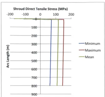
stress . . . . 75
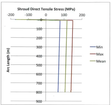
6-4 Reference well - OrcaFlex results - Uniform current and pen - Shroud deflection 76 6-5 Reference well - OrcaFlex results - Uniform current and pen - Tensile stress . . 76
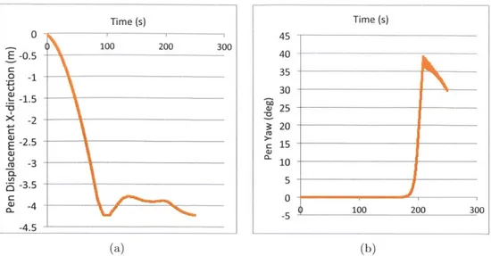
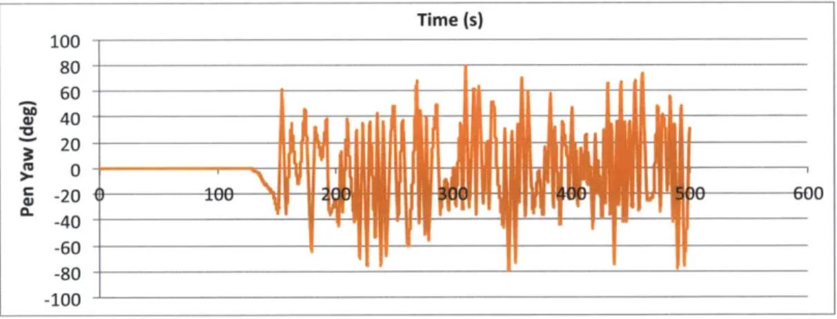
6-6 Reference well - OrcaFlex results - Uniform current and pen - Displacement and yaw of pen . . . . 77
6-7 Reference well -OrcaFlex results -Non-uniform current -Shroud displacement and tensile stress ... ... 78
6-8 Reference well - OrcaFlex results - Monochromatic wave -Deflection and tensile stress . . . . 79
6-9 Reference well -OrcaFlex results - Monochromatic wave -Shroud top displace-ment... ... 79
6-10 Reference well - OrcaFlex results -Monochromatic wave and pen - Deflections 80 6-11 Reference well - OrcaFlex results - Monochromatic wave and pen - Tensile stress 81 6-12 Reference well - OrcaFlex results - Monochromatic wave and pen - Shroud top displacem ent . . . . 81
6-13 Reference well - OrcaFlex results -Monochromatic wave and pen - Yaw of pen 81 6-14 Reference well - OrcaFlex results - Monochromatic wave and uniform current -D isplacem ents . . . . 82
6-15 Reference well - OrcaFlex results - Monochromatic wave and uniform current -Tensile stress . . . . 83
6-16 Reference well - OrcaFlex results - Monochromatic wave and uniform current -Top displacem ent . . . . 83
6-17 Reference well - OrcaFlex results - Monochromatic wave and uniform current with pen - Top displacement . . . . 83
6-18 Reference well - OrcaFlex results - Monochromatic wave and uniform current with pen - Displacements . . . . 84
6-19 Reference well - OrcaFlex results - Monochromatic wave and uniform current with pen - Yaw pen . . . . 84
6-20 OrcaFlex JONSWAP spectrum . . . . 87
6-21 OrcaFlex directional spectrum . . . . 87
6-22 Reference well - OrcaFlex results - Spectrum and current with pen -Roll . . 87
6-23 Reference well - OrcaFlex results - Spectrum and current with pen -Yaw . . 88
6-24 Reference well - OrcaFlex results - Wave spectrum and uniform current with pen - Displacements and stress profiles . . . . 88
6-25 Kevlar fatigue behavior . . . . 91
7-1 Mooring (line) design and deployment . . . . 95
7-2 Deployment step 1- Mooring lines/blocks . . . . 96
7-3 Deployment of bottom mooring . . . . 96
7-4 Mooring configuration for the reference well system . . . . 97
7-5 Deployment of the flared section . . . . 98
7-6 Connecting the flared section to a regular section . . . . 98
7-8 7-9 7-10 7-11 7-12 7-13 8-1 8-2 8-3 8-4 8-5 8-6 8-7 8-8
Way of connecting the mooring lines . . . . Connecting the mooring lines . . . . Connecting the pen . . . . Positioning the system . . . . Unfold the top most shroud section . . . . Final configuration . . . . Bubble/droplet diameters modeled for the Macondo well . . . . Macondo concentrations through the shroud . . . . Curves showing hydrate formation conditions . . . . OrcaFlex representation of realistic currents in the Gulf of Mexico Macondo well - OrcaFlex results - Uniform current . . . .
Macondo well - OrcaFlex results - Uniform current with pen . . . .
Macondo well -OrcaFlex results - Uniform current . . . . Macondo well -OrcaFlex results - Non-uniform current with pen .
8-9 Macondo well - OrcaFlex results - Monochromatic wave - Deflections . . . 122
8-10 Macondo well - OrcaFlex results - Monochromatic wave - Tensile stress . . . . 123
8-11 Macondo well - OrcaFlex results - Monochromatic wave - Shroud top deflection over tim e . . . 123
8-12 Macondo well - OrcaFlex results - Monochromatic wave with pen - Deflections 124 8-13 Macondo well - OrcaFlex results - Monochromatic wave with pen - Tensile stress124 8-14 Macondo well - OrcaFlex results - Monochromatic wave with pen - Shroud top deflection ... ... 125
8-15 Macondo well - OrcaFlex results - Monochromatic wave with pen - Roll and yaw of the pen . . . 125
8-16 Macondo well -OrcaFlex results - Monochromatic wave and uniform current -D eflections . . . 126
8-17 Macondo well - OrcaFlex results - Monochromatic wave and uniform current -Tensile stress . . . 126
8-18 Macondo well - OrcaFlex results - Monochromatic wave and uniform current -Shroud top deflection over time . . . 127
8-19 Macondo well - OrcaFlex results - Monochromatic wave and uniform current with pen - Deflections . . . 127
8-20 Macondo well - OrcaFlex results - Monochromatic wave and uniform current with pen - Tensile stress . . . 127
8-21 Macondo well - OrcaFlex results - Monochromatic wave and uniform current with pen - Shroud top deflection . . . 128
8-22 Macondo well - OrcaFlex results - Monochromatic wave and uniform current with pen - Pen roll and yaw . . . 128
8-23 Wave spectrum representing wave conditions at Macondo well . . . 129
8-24 Wave spectrum representing wave conditions at Macondo well . . . 129
8-25 Macondo well - OrcaFlex results - Wave spectrum and uniform current with pen - Deflections and tensile stress . . . 130
. . . 100 . . . 101 . . . 102 . . . 103 . . . 103 . . . 104 . . . 111 . . . 111 .. ... 112 .. ... 117 . . . 119 . . . 120 . . . 121 . . . 121
8-26 Macondo well - OrcaFlex results - Wave spectrum and uniform current pen - Pen roll and pitch over time . . . . 8-27 Macondo well - OrcaFlex results - Wave spectrum and uniform current pen - Pen yaw over time . . . .
with with
Overview of benchmarking categories . . . . Example of a capping stack . . . . Patented capping stack system . . . . Example of a soft seal system . . . .
Patents (a) W02011143276 and (b) W02012022277 Patent (a) unknown and (b) W02012007357 . . . . . Patents (a) JP2012007316 and (b) US2011297386 . .
Patent US2012006568 . . . . A-1 A-2 A-3 A-4 A-5 A-6 A-7 A-8 . 130 . 130 139 139 141 141 151 151 152 152 . . . . . . . . . . . . . . . . . . . . . . . . . . . . . . . .
List of Tables
1.1 Environmental conditions for the reference and Macondo well . . . . 19
2.1 F low data . . . . 25
3.1 Reference well vs Deep Spill . . . . 30
3.2 Bubble/droplet D50 for the reference well . . . . 31
3.3 Reference well plume data . . . . 34
4.1 R ib dim ensions . . . . 42
5.1 Depth-averaged flow parameters for the reference well . . . . 54
5.2 Gas concentrations compared to flammable limits . . . . 56
5.3 Gas concentration data for reference well . . . . 58
5.4 Hydrate volume as a % of shroud flow . . . . 59
5.5 Reference well -Results of the structural calculations . . . . 63
5.6 Structural sensitivity to design parameters . . . . 63
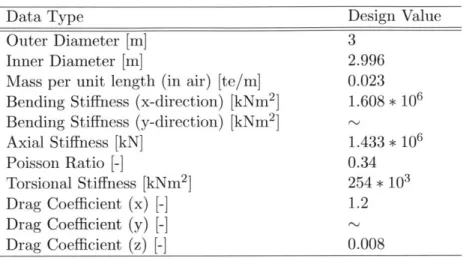
6.1 Reference well - OrcaFlex shroud line data . . . . 68
6.2 Reference well - OrcaFlex shroud mooring chain data . . . . 69
6.3 OrcaFlex modeling steps . . . . 73
6.4 Reference well - OrcaFlex data . . . . 74
6.5 Reference well - OrcaFlex results - Uniform current . . . . 75
6.6 Reference well - OrcaFlex results - Uniform current with pen . . . . 76
6.7 Reference well - OrcaFlex results - Non-uniform current (and pen) . . . . 77
6.8 Reference well - OrcaFlex results - Monochromatic wave . . . . 78
6.9 Reference well - OrcaFlex results - Monochromatic wave and pen . . . . 80
6.10 Reference well - OrcaFlex results - Monochromatic wave and uniform current (w ith pen) . . . . 82
6.11 Monochromatic wave characteristics measured at the reference well . . . . 85
6.12 JONSWAP parameter for OrcaFlex . . . . 86
6.13 Reference well input data for VIVA . . . . 91
6.14 Reference well output data for VIVA -Non-uniform current . . . . 92
8.1 Macondo well - Recap environmental conditions . . . 107
8.2 Macondo well - Flow data . . . 108
8.4 Macondo well -Depth-averaged flow parameters . . . 110
8.5 Macondo well - Gas concentrations vs. flammability thresholds . . . 112
8.6 Macondo well - Gas concentrations as % of saturation concentration . . . 113
8.7 Macondo well - Hydrate volume as % of flow . . . 113
8.8 Macondo well - Results of structural calculations . . . 114
8.9 Macondo well - OrcaFlex input data . . . 117
8.10 Macondo well - OrcaFlex results - Uniform current (with pen) . . . 119
8.11 Macondo well - OrcaFlex results - Non-uniform current (with pen) . . . 120
8.12 Macondo well - OrcaFlex results - Monochromatic wave . . . 122
8.13 Macondo well - OrcaFlex results - Monochromatic wave with pen . . . 124
8.14 Macondo well - OrcaFlex results - Monochromatic wave and uniform current (w ith pen) . . . 126
8.15 Macondo well - OrcaFlex results - Spectral wave and uniform current with pen 129 8.16 Macondo well - Output data for VIVA - Non-Uniform Current . . . 132
Chapter 1
Introduction
1.1
Background
The difficulty of capping the Macondo well blowout and the consequential environmental ef-fects have emphasized the need to find better response programs for the future. In order to reduce the environmental effect of the spill, the industry-wide preferred approach is to cap the well and stop the blowout. Since this is not always possible, other strategies have to be devised to cope with living subsea blowouts. There are two high level approaches available: dispersing the hydrocarbons using chemical dispersants or containing the hydrocarbons and then guiding them up to the surface. Attempts to contain the Macondo spill (and others) included a combi-nation of the two, partially due to a failure of the containment systems. Since then a number of research institutions have investigated the behavior of free hydrocarbon plumes (Socolofsky
et al., 2011) and the influence of dispersants (Brandrik et al., 2013), (Johansen et al., 2013). In
parallel to that a preference to contain the hydrocarbons rather than diluting them, has since led to the development of an extensive range of containment systems. These systems can be categorized into sealed (no interaction of hydrocarbons and ambient seawater, including cap-ping stack-like systems that rest on a BOP or cofferdam-like systems that rest on seabed) or non-sealed (off the seabed) systems that then can either be flexible or not (Appendix A). The
advantage of the sealed system is the conformity with the drilling standards and their ability to disconnect the top facility. However, important disadvantages include high weight, lack of oil water separation, need for accurate positioning and minimal dilution of gas concentrations.
The design presented here is a different (and new) kind of containment system, based on a passively induced chimney effect as working principle. Lessons learned from the problems with BPs cofferdam and the previously mentioned advantages for a containment system are
included into the design concept, on which the next paragraph will elaborate.
1.2
Concept
The proposed design is a lightweight, flexible structure with the ability to capture at least 90% of the spilled hydrocarbons during an expected lifetime of approximately six months. The buoyancy of the oil and gas creates a chimney effect, which is the working principle of this
system. The design ensures that the hydrocarbons are contained as they rise to the surface, see Figure 1-1. Since the chimney effect causes a pressure difference between interior and exterior of the shroud, this leads to a contraction of the shroud walls. Reinforcement ribs spaced approximately every ten meters constrain this narrowing of the internal cross-section.
owme skknr wWir
Shroud Section
Figure 1-1: Shroud concept
The shroud is stored onshore, ready to serve any number of offshore wells. In order for the system to fit the conditions at different wells, the design has a modular character built up of 100m identical sections. The deepest section is short and flared; the latter attribute guarantees the capture of the hydrocarbons from both a distributed as well as a point source. In order to generate the chimney effect the shroud extends from about 20 meters above the seafloor to approximately 10 meters below sea level. A big advantage of designing the system this way is that the shroud has a minimal impact on any work going on at the wellhead. Moreover, the majority of the deployment steps are performed from the water surface at a location offset from the wellhead, therefore reducing safety risks.
During installation a crane lowers the shroud sections through the moon pool of a multi-purpose vessel, starting with the flared bottom and consecutively adding on sections as the rest is lowered. Therefore each of the sections has a positive wet weight (in order to sink), but an air can mounted to the top section gives the total design a negative wet weight and keeps the shroud under tension. ROV's guide the shroud as it is lowered and finally they connect the bottom mooring lines that are already connected to ballast blocks, to the flared section.
At the surface a deep, circular pen collects the hydrocarbons. It is designed to hold a satisfactory volume, withstand wave motions, and promote the separation of the oil droplets from the water exiting the shroud. A secondary pen could be used as a backup to contain whatever small quantities of oil that escape the primary pen due to, e.g., extreme weather.
1.3
Design Cases
One of the fundamental design principles is the modularity of the system so that it can operate on a large range of wells. One system can therefore serve a large geographical region, e.g. the Gulf of Mexico. To achieve this multipurpose system, the design process includes two dis-tinct sites; together they will generate a design that can function in a combination of extreme conditions. The first is a well of interest to the sponsor (that is not yet in use), hereafter referred to as the 'reference well'. The conditions at this well are relatively mild (Exploration
and Division, 2011). The other is the Macondo well in the Gulf of Mexico (see Figure 1-2),
where the conditions are much more demanding (Camilli et al., 2011) and the well has a flow rate that represents the larger wells operating today. Chapter 2 presents further data.
Figure 1-2: Location of the Macondo well in the Gulf of Mexico
Table 1.1: Environmental conditions for the reference and Macondo well
Parameter Water Depth
Typical Current Bottom Temperature Significant Wave Height Peak Wave Period Oil Flow Rate
Gas Flow Rate (at well)
Reference well 830m 0.1 m/s 130C 0.1 -2.5m 2 - 8.5s 0.015 m3/s 0.0028 Am3/s Macondo well 1500m 0.1 m/s 40C 1.0 - 2.7m 6 - 7.5s 0.10 m3/s 0.09 Am3/s
From this point the analysis proceeds to look insight into consequences of introducing the full description of the shroud compartments,
into the behavior of a free blowout plume to get shroud system. After that Chapter 4 gives the
with their chosen dimensions. The next section goes on to describe analytical analysis on the fluid mechanics in and around the shroud, as well as primary structural analysis. Chapter 6 then describes the use of the software tool OrcaFlex to model the shroud response to different, more complex environmental conditions. That is the last stage of the design and analysis phase for the reference well. Before moving on to describe the installation and validation (future work), Chapter 8 will discuss the small variations to the design parameters for the system to operate for the Macondo well conditions as well.
Chapter
2
Data Design Cases
The design process for the shroud requires a range of data about the environmental as well as flow conditions associated with the respective wells. This section presents all the data needed for the further analysis per topic for both the reference and the Macondo well.
2.1
Environmental Data
2.1.1 Reference Well
This data set refers to the ambient conditions such as water temperature and salinity, water density (Trieste) and the currents (Poulain et al., 1996).
Salinity profile Salinity (gm/kg) 37.4 37.6 37.8 38 38.2 38.4 38.6 38.8 0 100 200 300 400 joo600 700 800 900 (a)
Figure 2-1: Salinity (a) ence well (Trieste).
Temperature profile 0 100 200 300 S400 500 600 700 800 900 Seawater Temperature ( C) 13 14 15 16 17 18 19 20 21 22 23 24 --- --- _ _ _
Ii
-Winter -Spring -Summer -Autumn-2 per. Mov. Avg. (Spring)
(b)
and temperature (b) profiles measured at the
refer-The degree of ambient stratification and the strength of the currents are factors that influ-ence the behavior of the hydrocarbon plume and/or the shroud. Figures 2-1 and 2-2 indicate a moderate density change over depth, without any strong stratification.
-Density profiles for the 4 seasons Density (kg/mA3) 1025.5 1026.0 1026.5 1027.0 1027.5 1028.0 1028.5 1029.0 1029.5 0 100 200- ---Summer 300 -Winter 40 ---Spring 500 .Autumn 600 800 9 0 0 - - - --
-Figure 2-2: Water density profile at the reference well.
As shown in Figure 2-3 both the magnitude and the direction of the currents change over depth and throughout the year. The absolute magnitudes are generally less than 0.1 m/s and they rarely exceed 0.2m/s at any given time of the year. Hence 0.1 m/s is used as a typical current and 0.2 m/s is used as a design current for calculating drag forces. It can also be noted that the direction of the current over depth changes strongly over the year. Consequently, during some seasons the current is close to uniform over depth (causing a high net drag force), while in other seasons the current direction changes up to 180 degrees over depth (giving rise to a smaller net drag force on the shroud).
Current speed (m/s)
S-0.1 -0.05 0 0.05 0.1 0.15
-Summer Current -Feb-95
Figure 2-3: Current profiles at the reference well site for the different seasons. Two sources were used.
2.1.2 Macondo Well
For the Macondo well the temperature and density profiles (Figure 2-4) originate directly from the NOAA Buoy Data Center (NOAA, 2012) and Socolofsky et al. (2011) respectively. The current profile (Figure 2-5) is obtained from a report on the currents in the Gulf of Mexico for the US Department of Interior.
Since the shroud only reaches to within several meters of the sea surface, the design is tested on a
0.2m/s
current. This value is considered a good depth- and time-average (yearly average).Water temperature (degrees Celcius)
) 5 10 15 20 25 30
(a)
Figure 2-4: (a) Temperature and
(Socolofsky et al., 2011)
Water Density (kg/mA3) 1026.6 1026.8 1027 1027.2 1027.4 1027.6 1027.8 200 E 400 - 600 4 800 41000 1200 1400 1600 (b)
(b) density profiles for the Macondo well
Current speed (m/s) 0 0.1 0.2 0.3 0.4 0.5 0.6 0 200 . 400 600 0. 800 1000 1200 1400 C-May -December
Figure 2-5: Current profiles for the the Macondo well for two months showing
two extreme conditions Sturges et al. (2004)
2.1.3
Surface Tension
Oil droplet behavior requires data on the surface tension between the hydrocarbons and the water
" Surface tension Oil - Water: 0.025 kg/s2 (Federal Interagency Solutions Group and
Team, 2010)
" Surface tension Gas - Water: 0.055 kg/s2 (Sacks and Meyn, 1995)
0. 0-200 400 600 800 1000 1200 1400 1600
2.2
Flow Data
2.2.1
Outlet Diameter
We are interested in the diameter of the outlet because its dimensions influence the size of the bubbles/droplets that will create the hydrocarbon plume. In the case of the reference well, three outlet diameters for the blowout jet are to be considered according to ENI S.p.A.:
* 5" 0.13m
* 9" 0.23m
* 18" ~ 0.46m
For the calculations here we focus on the smallest outlet with an opening of 0.13m, due to its similarity to the 0.12m opening used for the Deep Spill experiment (Johansen, 2001), which operates as a reference to check calculations. Furthermore the smaller opening size causes the bubbles to be more in the atomized range, which means that they will have a smaller slip velocity. A low slip velocity causes the free plume to be more influenced by a cross current to become trapped by ambient stratification at a level of neutral buoyancy.
For the Macondo well observations suggest that the effective diameter of the broken riser through which the oil spilled in the initial weeks, was approximately 42cm (Camilli et al., 2011). After the riser was cut the effective diameter was about 49cm. We will use the 42cm diameter in combination with estimated flow rate found by Camilli et al. (2011) to calculate the bubble and droplet diameters in Chapter 4.
2.2.2 Hydrocarbon Flow Data
Table 2.1 presents data for the oil wells, providing further detail on the oil/gas flow and their characteristics for the reference (Exploration and Division, 2011) and Macondo well (Camilli
et al., 2011). Two types of units are used for the flow rate; Am3/s is used for the flow rate
measured at the well head (under local pressure and temperature) and Sm3/s as units for the
flow rate under Standard conditions (atmospheric pressure and temperature of 293K). The difference is needed due to the large density change that gasses undergo between deep ocean conditions (large pressure and low temperature) to atmospheric conditions.
The dissimilarities between the gas flow rates at the well head and the surface at each site are due to volume expansion and gas that is dissolved in the oil at the well head but comes out of solution during its ascent. Given the oil/gas composition in Table 2.1 the contribution of the components other than methane, ethane or propane are neglected in the analysis for the shroud design.
Table 2.1: Hydrocarbon flow data
Parameter Reference well Macondo well
Oil
- Flow rate 0.015 Am3
/s
0.10 m3/s- Density 761.7 kg/M3 858 kg/M3
Gas
At the well head
- Flow rate 0.0028 Am3/s 0.09 Am3/s
- Density 95 kg/M3 120 kg/m 3s
At the surface
- Flow rate 1.435 Sm3/s 31 Sm3/s
(0.014 m3/s at the bottom) (0.162 m3/s at the bottom)
- Density 0.82 kg/M3 0.73 kg/m 3s Composition (mol %) - Methane 87.4 82.5 - Ethane 7.1 8.3 - Propane 2.1 5.3 - Others 3.4 3.9 Total 100% 100%
Chapter 3
Free Blowout Plume
The analysis of the free plume can be compared to the use of a control study; before moving on to the shroud design it is important to understand what the behavior of the hydrocarbons is without any interference. Will the environmental conditions cause the plume to stratify or will it rise as a coherent plume? Other points of interest are the location at which the hydrocarbons surface and what percentage that is of the total released volume. The first step is to determine the bubble and droplet diameter, after which we can analyze the global plume behavior, since the rise velocity of individual bubbles and droplets depends on their size. From the individual behavior of the bubbles and droplets we can consequently determine the gas (and oil) concentrations at the surface. These concentrations are important, because they need to satisfy industry requirements with respect to workers safety. This analysis is only done for the reference well.
3.1
Bubble and Droplet Size
There are at least three reasons why it is necessary to know the individual bubble/droplet sizes:
* Size influences the effect that stratification and cross current have on the free plume
" Workers' safety is related to surface gas concentrations, which depend on gas dissolution
rates, which in turn depend on bubble diameter.
" Oil droplet size helps determine whether the oil and water will separate after exiting the
shroud, which then influences the required pen size.
3.1.1 General Theory
The starting point to calculate the size of the droplets and bubbles is the outlet diameter of the wellhead. The equivalent diameter of this nozzle, together with the flow rate of the jet velocity, govern the initial stable size of the bubbles and droplets. A higher jet velocity is as-sociated with smaller droplets/bubbles (atomization), while larger outlet diameters produce large droplets/bubbles. The initial diameter is then reduced to a smaller, stable diameter based on a balance between turbulent kinetic energy tending to break up the bubbles and
droplets and surface tension tending to stabilize them. For low values of surface tension, as would occur when chemical dispersants are used, viscosity can also help stabilize droplets and bubbles (Johansen et al., 2013). Once the bubbles/droplets reach the bottom of the shroud they have already obtained a diameter equal to or smaller than the critical diameter. As they ascend further, dissolution and volume expansion are competing effects influencing the diameter of the droplets/bubbles. The net of the two effects combined determines the change in diameter of the droplets/bubbles as they travel up through the shroud. The turbulent flow in the shroud will not affect them, since the diameters are already equal to or smaller than the critical value.
Johansen et al. (2013), as part of SINTEF, developed a model that finds a volume
me-dian droplet size D5 0, so half of the volume is in the form of droplets/bubbles with a smaller
diameter. On the basis of this characteristic diameter various models exist to find the di-ameter distribution; here we use the Rosin-Rammler model. Under stationary conditions the characteristic bubble/droplet size (D50 here) is defined by
D5 0 = c ( ) 3/5 E2/5
(3.1)
\PW/
where a and pw are the surface tension and water density, E is the fluid turbulent dissipation rate and c is a constant. In a turbulent jet, like in our case, the bubbles and droplets experience a time varying turbulent energy, whose magnitude scales as
U3
E ~ 3(3.2)
Dj
Name Unit Description
Pw kg/n 3 Density of the water ~ 1028kg/m 3
- kg/s 2 Surface tension
E m4 /s2 Fluid turbulent dissipation rate
U m/s Jet velocity
D3 m Jet diameter
Combining Equations 3.1 and 3.2 leads to Equation 3.3 for D5 0.
D5 0 - A Dj We-3/ 5 (3.3)
where We is the Weber number, which is defined as in Equation 3.4 and A is an empirical constant.
For small surface tension, viscosity becomes important and We is replaced by We*:
W e
We* = We(3.5)
1 + B Vi (D50/Dj) 1/3
where Vi represents the viscosity (pU/-, where u is the dynamic viscosity). Viscosity be-comes important when chemical dispersants are used to reduce the surface tension, but in our case the surface tension is relatively large, therefore overpowering the importance of viscosity, which means that we do not need to use the modified Weber number to find D5 0.
The above theory is based on a two phase jet in which a single dispersant phase (oil) is discharged into a second continuous fluid; however in the case of an oil spill the jet is often a mix of oil and gas. The heterogeneity of the fluid affects the break-up dynamics in two ways. Firstly, due to the much smaller density of the gas relatively to the oil, it forces the oil to flow through a smaller cross-sectional area of the orifice. Secondly, due to the high buoyancy of the gas, the discharge of the heterogeneous fluid is going to behave more like a plume. Following Johansen et al. (2013), the first effect can be accounted for here by defining
a nominal velocity as in Equation 3.6 and an effective orifice diameter D' (Equation 3.7), for the oil or gas through the orifice, where 0 is the void fraction occupied by the gas. The nominal velocity is associated with a jet of only oil droplets or gas bubbles that has the same kinematic momentum as the jet with both oil and gas.The nominal velocity can then be used to find the nominal value of the Weber number, in order to define the D5 0 associated with the
heterogeneous jet.
Uj
Un = Ui (3.6)
D' = D f(1 -n) (3.7)
The second effect is accounted for by further modifying the jet exit velocity so that it has the same velocity as a buoyant jet at a characteristic distance from the orifice which is known as the momentum length. Again, following Johansen et al. (2013), this velocity is given by
Uc = U, (1 + Fr-1 ) (3.8)
where Fr is the densimetric Froud number, which is defined as follows
Fr = Un(3.9)
VlD g[pw - p(l - n)]/p(
By combining Equations 3.6, 3.8, 3.9 and 3.4 we can determine D5 0 by using Uc in Equa-tion 3.3.
As mentioned before, coefficients A and B are empirical coefficients. In absence of the viscosity dependence like in our case, Equation 3.3 only has A as an empirical coefficient. The predicted value of D5 0, therefore, becomes directly dependent on the value of A. Brandrik
Johansen et al. (2013) found A = 15 (and B = 0.8) for experiments also involving only with
oil. In experiments where the oil viscosity plays a role, the chosen value for A can be balanced out by a certain choice for B. Since this is not possible in our case, we needed to calibrate the model in a different way. A deep spill experiment off the coast of Norway in 2000 had very similar conditions to those of the reference well as can be seen in Table 3.1 (Johansen, 2001); therefore observational data from that experiment can be used to calibrate a right value of A for our model. This value for A can then be used to predict the D5 0 for both the reference
and Macondo well.
Table 3.1: Comparison of the reference well data to data from the Deep Spill experiment
Water depth (m) Currents (m/s) Jet diameter (M) Oil flow rate (m3/s)
Gas flow rate (m3/s)
Reference well 830 0.1 0.13m 0.015 0.0028
The observed bubble and droplet distributions for the Deep Spill experiment are shown in Figure 3-1, from which we can compare the values for D5 0 with our calculated values.
Observed See Bubbe Volume
__*a__uion
I I
04
02
0.1 0.2 03 0A 03 *A 0. 7 0 OS 10 1.1 L2 13 L
Figure 3-1: (a) Gas bubble and (b) at the Deep Spill experiment
Observed OIl Drplet Volume
Dbbtibution
01 02 03 04 05 07 0 0 t0 1A 11 12 1.3 14
oil droplet distributions (in cm) observed
The observed D50's are:
"
Bubble D5 0: 0.0047m* Droplet D5 0: 0.0044m
Using the model described before, neglecting the viscosity term and using the water density to calculate the Weber number, we find that the 'correct' value for A in our model is 18.7. Using this value we predict the same values for the D50's as were observed.
Based on the D50's we can find the cumulative volume distribution using the
Rosin-Rammler model [Equation 3.10], which is defined by the following equation, where n is a Deep Spill 840 0.1 0.12m 0.017 0.007
fitting parameter. The value of n has a non-negligible affect on the found distribution, but
Bailey et al. (1983) found that values of
n
> 3 produce good results.V(D) = 1 - exp[-0.693(D/D50)'] (3.10)
For this research the value of n is validated by fitting it to observed bubble and droplet diameter data for an oil spill with comparable conditions (SINTEF's Deep Spill Experiment
(Johansen, 2001))
The following two paragraphs discuss the results from the models to find the bubble and droplet distributions for the reference and Macondo well respectively.
3.1.2 Reference Well
As mentioned in Chapter 2.2.1, for the reference well we work with a 13cm jet diameter. For this diameter, the given oil and gas cha'racteristics and the value for the coefficient A (in Equation 3.3), the characteristic bubble and droplet diameters can be determined. The results are presented in Table 3.2.
Table 3.2: 50% bubbles/droplets for the reference well
Input [Output
Jet diameter 0.13m Gas D50 0.0043m
Jet velocity 1.34m/s Oil D5 0 0.0064m
Coefficient A 15
Surface tension 0.025kg/s (Oil)
0.055kg/s (Gas)
Since we were able to calibrate the SINTEF model (using coefficient A) to fit the observed data, we will use the SINTEF model to predict the bubble and droplet sizes exiting the well (Figure 3-2).
Gas bubble and Oil droplet distribution for the reference well
1i I E 0 E E U 0.8 0.6 0.4 0.2 r'0 0.005 0.01 0.015 Bubble/Droplet diameter (m) 0.02 Figure 3-2: Predicted (a)
for the reference well
gas bubble and (b) oil droplet distributions (in cm) -Bubble distribution
3.1.3
Macondo Well
The general model described earlier can also be used to describe a bubble/droplet distribution for the Macondo well. The input parameters are the following:
" Rossin-Ramler fitting parameter n = 3
* Gas fraction (n) = 0.43
" Jet diameter 0.42m (observed equivalent diameter for the broken riser)
* Jet Velocity 1.5m/s
As mentioned before, the fitting (spreading) parameter can be chosen to be any value equal to or larger than 3. Unfortunately there is no data to which we can fit the distribution for this case, so for continuity n is kept at 3. The SINTEF model, with A = 18.7, gives the following values for the critical diameters:
* Gas bubbles; D50 = 0.0088m
" Oil droplets; D50 = 0.0072m
Using the Rossin-Rammler equation (3.10) we can use the D5 0's to determine the volume
distributions. These bubble and droplet distributions are presented in Figure 3-3.
Gas bubble and Oil droplet distribution Macondo
1 a>
0.8
E > 0.6 0.4 E E 0 0.2--Bubble distribution --Droplet distribution] 0 0.005 0.01 0.015 0.02 0.025 Bubble/Droplet diameter (m)Figure 3-3: Modeled bubble/droplet distribution for the Macondo well
The SINTEF model has two important uncertainties to be aware of: firstly, should the Weber number be calculated using the density of water or the density of the dispersed phase (oil), and secondly, what are the values for coefficients A (and B). The first issue is still a point of discussion in the field of droplet dynamics. The effect of oil versus water density is small (and can be accounted for in the coefficient A), but the effect of gas versus water density is huge. For this reason we used the water density. We have tried to address the
second uncertainty by calibrating it to observed data from the Deep Spill Experiment. Re-gardless of these uncertainties, the SINTEF model is the best that is currently available to predict bubble/droplet diameters in a multi-phase jet, which is why we decided to work with it.
3.2
Free Plume Behavior for the Reference Well
There are two idealized multiphase plume behaviors: stratified dominated or current domi-nated. The difference between these global behaviors indicates how the hydrocarbons rise to the surface. Which of the two behaviors will dominate depends on the relative magnitude of the peel height (hp) and the separation height (hs); both depend on the buoyancy flux and the rise velocity of the bubbles/droplets. See Figure 3-4 for the definitions of both heights
(Socolofsky et al., 2011).
h . * ..
(a)
Figure 3-4: Free plume behavior; (b) current dominated (hp > h,) Parameter Buoyancy flux Buoyancy frequency Separation height Peel height 10 00 0000 0 00 00 00 0 00 0O 0. 0 00 0 0 0 00. 0 0:. 0 0 0 U0 0 0 .0 000 0 00
~0
h8%00 0 (b)0'*
(a)~~~0 staiiaindmntd(0< 0 n Equation Bo Qo(pa - P)/Pr N =-g/prOpa/&z) h= 5.1BO/(Uu/24)0.88 hp/(Bo/N3). = 5.2exp[-(uS/(Bo/N)' .)/01For the buoyancy frequency we use a linear approximation of the density profile for 9pa/Dz. In order to find inclusive results, the buoyancy frequency was calculated for the summer and winter conditions, which have the steepest slope of water density over depth. Furthermore, for the calculations of the separation and peel height the slip velocities used are those for the largest and smallest diameter bubble/droplet, which range from 0.10 - 0.21m/s (Zheng and
For the reference well the peel height is bigger than the separation height under all circum-stances (Table 3.3), which implies a strongly current dominated behavior. Consequently, most of the hydrocarbons in a free plume will surface downstream of the blowout (Figure 3-5).The horizontal distance from the well to the surface location of the hydrocarbons depends on the slip velocity (which depends on the droplet/bubble size) relative to the current speed. For the bubble and droplet sizes described in Section 3.1.2 with rise velocities between 0.1 and 0.21 m/s, and a current speed of 0.1 m/s, it is found that the hydrocarbons from the reference well would surface between 1200m and 3600m downstream from the wellhead.
Table 3.3: Reference well free plume separation and trap height
Parameter Reference well
Buoyancy flux (m4/s3) 0.062
Buoyancy frequency (1/s) Winter: 0.000833
Summer: 0.001
Separation height (M) Biggest bubble/droplet: 65
Smallest bubble/droplet: 254
Peel height (M) Winter: 554
Summer: 452
U=0.1m ISS
ee*
h,=65m
Figure 3-5: Predicted current dominated blowout plume under the reference well conditions
3.3
Gas Dissolution
During their ascent to the surface the bubbles and droplets will partially dissolve due to mass transfer into the ambient water. It is important to understand the change in gas volume during the rise of the bubbles to the surface, because gas concentrations at the surface need to be below flammable thresholds. Of oil droplets generally there is negligible mass transfer, the dissolution calculations therefore focus on the gas bubbles.
Two competing mechanisms influence the change in total volume of the gas bubbles over depth; gas dissolution will decrease the bubble volume as it ascends towards the surface, while volume expansion results from a reduction in hydrostatic pressure. The combined effect is
described as the change of diameter for individual bubbles of a given starting diameter. Hirai
et al. (1996) found that this behavior is expressed by the equation:
dD 2kS dpD (3.11)
dz UzP dz 3p
Name Unit Description
k m/s Mass transfer coefficient
S kg/M3 Solubility of the gas in (sea) water
p kg/M3 Density of the gas at ambient pressure/temp
D m Bubble diameter
UZ
m/s Rise velocity of the bubbles (which will be a combination ofthe slip velocity and the velocity of the water-hydrocarbon mixture through the shroud)
The first term in the equation represents the mass transfer, which depends on the diffusivity and solubility of the gas in the ambient water (since the gas concentration in the ambient water is considered negligible). The mass transfer depends on the diffusivity in the following way (Johansen, 2004):
k = Sh (3.12)
D
In which the Sherwood number is defined as follows:
2 2.89
Sh = 1 - vPe (3.13)
/7F _ Re
in which K (m2/s) is the molecular diffusivity of the solute in the water,
Sh
is the Sherwood number, Pe = wD/K is the Peclet number (where w is the slip velocity), and Re is the Reynolds number.The second term in Equation 3.11 accounts for the volume expansion of the bubble due to the reducing hydrostatic pressure during the ascent. The reduction in pressure causes a change in densities of the gasses over the water depth. The way the density changes over depth is defined by the Peng-Robinson equation of state (McCain, 1990):
[+
a (Vm - b) = RT (3.14)Name Unit Description
p N/m 2 Pressure
Vm m3/mol Molar volume
R J/K/mol Universal gas constant
T K Absolute temperature
aT - Coefficient
b - Coefficient
Most of the parameters in Equation 3.11 -Equation 3.14 are component specific; therefore the calculations are done for bubbles of pure methane, ethane or propane separately. The total gas volume (0.0028 m3/s) is distributed over the individual components. The bubble
diameters then govern the number of bubbles for each of the gasses. Figure 3-6 shows the change of the bubble diameters over depth for the free plume.
Methane 0 100 200 300 400 500 600 700 800 0 0.01 0.02 Diameter of Bubble (m) Ethane 0 100 200 300 400 500 '. 600 700 800m r ( 0 0.01 0.02 Diameter of Buble (m) Propane 0 100 200 300 400. 500 600 700 800 0 0.01 0.02 Diameter of BLbble (m)
Figure 3-6: Reference well free plume predicted bubble diameter change over depth
The jumps in the curves for the ethane bubbles/droplets in Figure 3-6 indicate the depth at which the ethane transitions from liquid to gas. This phase change is accompanied by a large jump in the density. The results presented in Figure 3-6 show that all the methane bubbles, the smaller two-thirds of the ethane and all the propane bubbles can dissolve entirely. Based on this data the gas concentrations can be determined as a function of the water
depth (Figure 3-7).
The hydrocarbons exit the jet to form a free plume, which entrains a large volume of water as it rises. At the separation height the hydrocarbons leave the plume and rise as individual droplets to the surface. The conditions at the reference well result in a small separation height (relative to the water depth), which made it possible to calculate the concentrations based on the behavior of individual bubbles.
C SBuble Diameter =0.001 m SBuble Diameter =0.002 m Bubble Diameter =0.003 m Bubble Diameter =0.004 m Bubble Diameter =0.005 m Bubble Diameter =0.006 m Bubble Diameter =0.007 m * Bble Diameter =0.008 m Bubble Diameter =0.009 m * Bule Diameter =0.01 m SBuble Diameter =0.011 m SBuble Diameter =0.012 m
0
Methane 0 + + 100 2001 300 400 500 600 700 800 9 0 0 Ethane Propane 0 100 2001 300 9400
~500
600- 700-800 90 0 0 100 200 300 9400 B500 600 700 800 Soo0F
0.05 oil -- free gaslilquid -gas in oil-dissolved gas in water
+ solublity
Concentration Concentration Concentration
(ka/m3l (ko/m3) (kjlm3l
Figure 3-7: Reference well free plume predicted concentration change over depth
Similar calculation will be done in Sections 5.3 and 8.5 for the change of the bubble di-ameters and gas concentration during the ascent through the shroud, for the reference and Macondo well respectively.