Deep Neural Networks for Choice Analysis
by
Shenhao Wang
Submitted to the Department of Urban Studies and Planning
in partial fulfillment of the requirements for the degree of
Doctor of Philosophy in Computer and Urban Science
at the
MASSACHUSETTS INSTITUTE OF TECHNOLOGY
Feburary 2020
c
○ 2020 Massachusetts Institute of Technology. All rights reserved.
Author . . . .
Department of Urban Studies and Planning
September 13, 2019
Signed by . . . .
Jinhua Zhao
Edward H. and Joyce Linde Associate Professor
Department of Urban Studies and Planning
Supervisor
Accepted by . . . .
Jinhua Zhao
Edward H. and Joyce Linde Associate Professor
PhD Committee Chair
Department of Urban Studies and Planning
Deep Neural Networks for Choice Analysis
by
Shenhao Wang
Submitted to the Department of Urban Studies and Planning on September 13, 2019, in partial fulfillment of the
requirements for the degree of
Doctor of Philosophy in Computer and Urban Science
Abstract
As deep neural networks (DNNs) outperform classical discrete choice models (DCMs) in many empirical studies, one pressing question is how to reconcile them in the con-text of choice analysis. So far researchers mainly compare their prediction accuracy, treating them as completely different modeling methods. However, DNNs and classi-cal choice models are closely related and even complementary. This dissertation seeks to lay out a new foundation of using DNNs for choice analysis. It consists of three essays, which respectively tackle the issues of economic interpretation, architectural design, and robustness of DNNs by using classical utility theories.
Essay 1 demonstrates that DNNs can provide economic information as complete as the classical DCMs. The economic information includes choice predictions, choice probabilities, market shares, substitution patterns of alternatives, social welfare, prob-ability derivatives, elasticities, marginal rates of substitution (MRS), and heteroge-neous values of time (VOT). Unlike DCMs, DNNs can automatically learn the utility function and reveal behavioral patterns that are not prespecified by modelers. How-ever, the economic information from DNNs can be unreliable because the automatic learning capacity is associated with three challenges: high sensitivity to hyperparam-eters, model non-identification, and local irregularity. To demonstrate the strength of DNNs as well as the three issues, I conduct an empirical experiment by applying the DNNs to a stated preference survey and discuss successively the full list of economic information extracted from the DNNs.
Essay 2 designs a particular DNN architecture with alternative-specific utility functions (ASU-DNN) by using prior behavioral knowledge. Theoretically, ASU-DNN reduces the estimation error of fully connected DNN (F-DNN) because of its lighter architecture and sparser connectivity, although the constraint of alternative-specific utility could cause DNN to exhibit a larger approximation error. Both ASU-DNN and F-ASU-DNN can be treated as special cases of ASU-DNN architecture design guided by utility connectivity graph (UCG). Empirically, ASU-DNN has 2-3% higher prediction accuracy than F-DNN. The alternative-specific connectivity constraint, as a domain-knowledge-based regularization method, is more effective than other regularization methods. This essay demonstrates that prior behavioral knowledge can be used to
guide the architecture design of DNN, to function as an effective domain-knowledge-based regularization method, and to improve both the interpretability and predictive power of DNNs in choice analysis.
Essay 3 designs a theory-based residual neural network (TB-ResNet) with a two-stage training procedure, which synthesizes decision-making theories and DNNs in a linear manner. Three instances of TB-ResNets based on choice modeling (CM-ResNets), prospect theory (PT-(CM-ResNets), and hyperbolic discounting (HD-ResNets) are designed. Empirically, compared to the decision-making theories, the three in-stances of TB-ResNets predict significantly better in the out-of-sample test and be-come more interpretable owing to the rich utility function augmented by DNNs. Com-pared to the DNNs, the TB-ResNets predict better because the decision-making the-ories aid in localizing and regularizing the DNN models. TB-ResNets also become more robust than DNNs because the decision-making theories stablize the local utility function and the input gradients. This essay demonstrates that it is both feasible and desirable to combine the handcrafted utility theory and automatic utility specifica-tion, with joint improvement in predicspecifica-tion, interpretaspecifica-tion, and robustness.
Committee member: Stefanie Jegelka
Title: X-Consortium Career Development Associate Professor Electrical Engineering and Computer Science
Committee member: Drazen Prelec
Title: Professor of Management Science and Economics
Sloan Management School, Department of Economics, and Department of Brain and Cognitive Science.
Supervisor: Jinhua Zhao
Title: Edward H. and Joyce Linde Associate Professor Department of Urban Studies and Planning
Acknowledgments
I feel a great gratitude towards my advisor Jinhua Zhao. He guided me through every step in this PhD program. Jinhua provides me the freedom to explore different ideas. My research directions had two dramatic changes in the past five years: from a policy focus about five years ago, to a behavioral focus about two years ago, and to this current dissertation that strongly relies on machine learning models. This large interest shift would be impossible without Jinhua’s full support. Jinhua is not only a great advisor academically, but also taught me the skills in management and communication. It is very rare for any supervisor to provide the consistent and reliable support as Jinhua does. Words are not enough to express my gratitude towards Jinhua’s helps.
I am grateful for the concrete suggestions that Stefanie Jegelka gave for my dis-sertation. Stefanie suggested me to learn statistical learning theory, nonlinear and robust optimization about two years ago, taught me the network perspective in her class, and tested my skills about the DNN-related topics in my qualifying exams. Stefanie helped me to explore the machine learning path I did not know much about two and a half years ago. I feel so grateful that the best suggestions were given at an early stage of my dissertation writing.
I am grateful for Drazen Prelec’s helps. As a behavioral economist, Drazen helps me with the behavioral perspectives in the dissertation. I took Drazen’s behavioral economics class first time in 2015 and second time in 2017. It is the only class I took twice in MIT. Drazen helped me with a paper about risk and AV adoption, which I did not incorporate in this dissertation. I wish I could have incorporated more papers into this dissertation to show my gratefulness. It is always a pleasure to work with him.
I feel so lucky to be in MIT, with its nearly unique institutional culture encouraging creativity and interdisciplinary collaborations. This dissertation is a synthesis of diverse perspectives, and I fully understand that this synthesis would be impossible in most of the other institutions in the world. Besides the three committee members,
the faculties in MIT taught me great knowledge that contributes significantly to this dissertation. I learnt econometrics models from Jerry Hausman, demand modeling from Moshe Ben-Akiva, machine learning skills from the machine learning group in computer science, optimization skills from Bart Parys, statistical learning theory from Sasha Rakhlin, and a lot of knowledge in many other classes.
The micro-environment in JTL built by Jinhua is amazing. JTL members always provide very valuable and constructive comments on my studies. For my dissertation, I would like to thank Qingyi Wang for her consistent and effective modeling supports, particularly for the first essay. I am also grateful for the great comments, suggestions, and the proofreading helps from Nate Bailey, Joanna Moody, Mary Rose Fissinger, Jintai Li, Jeff Rosenblum, Fiona Tanuwidjaja, and many others I cannot name one by one.
The academic environment in DUSP provides a nearly unique opportunity for the birth of this dissertation because it allows the interaction of many diverse and even opposite views to interplay in one issue. I can also get great career, research, and life suggestions from the faculties in DUSP: Larry Susskind, David Hsu, and Larry Vale. I am also grateful for the daily supports from my classmates: Elise Harrington, Nick Kelly, and many others.
Lastly, I need to thank my mother and grandmother for their supports on my life. It is great that my mother did not force me to get married or to make big money in the past few years, but largely kept silence to allow me to pursue my interests. I know how difficult it is to refrain from taking actions, which is the virtue of self-control. The greatest thank-you is devoted to my father, who nurtured me to be a person with decent characters. I wish he can feel calm and ease in the heaven.
Contents
1 Introduction 15
1.1 Background . . . 15
1.2 Dissertation Overview . . . 18
2 Essay 1: Extracting Complete Economic Information for Interpre-tation 21 2.1 Introduction . . . 21
2.2 Literature Review . . . 23
2.3 Model . . . 27
2.3.1 DNNs for Choice Analysis . . . 27
2.3.2 Computing Economic Information From DNNs . . . 29
2.4 Setup of Experiments . . . 31
2.4.1 Hyperparameter Training . . . 31
2.4.2 Training with Fixed Hyperparameters . . . 32
2.4.3 Dataset . . . 32
2.5 Experimental Results . . . 33
2.5.1 Prediction Accuracy of Three Model Groups . . . 34
2.5.2 Function-Based Interpretation . . . 34
2.5.3 Gradient-Based Interpretation . . . 40
2.6 Discussions: Towards Reliable Economic Information from DNNs . . 45
3 Essay 2: Architectural Design with Alternative-Specific Utility
Func-tions 59
3.1 Introduction . . . 59
3.2 Literature Review . . . 62
3.3 Theory . . . 64
3.3.1 Random Utility Maximization and Deep Neural Network . . . 64
3.3.2 Architecture of ASU-DNN . . . 66
3.3.3 DNN Design Guided by Utility Connectivity Graph . . . 68
3.3.4 Estimation and Approximation Error Tradeoff Between ASU-DNN and F-ASU-DNN . . . 70
3.4 Setup of Experiments . . . 73
3.4.1 Datasets . . . 73
3.4.2 Hyperparameter Space and Searching . . . 74
3.5 Experiment Results . . . 75
3.5.1 Prediction Accuracy . . . 75
3.5.2 Alternative-Specific Connectivity Design and Other Regular-izations . . . 77
3.5.3 Interpretation of ASU-DNN . . . 80
3.6 Conclusion . . . 82
4 Essay 3: Theory-Based Deep Residual Neural Networks 89 4.1 Introduction . . . 89
4.2 Literature Review . . . 91
4.3 Theory . . . 94
4.3.1 Theory-Based Residual Neural Networks (TB-ResNets) . . . . 94
4.3.2 Three Instances of TB-ResNets . . . 96
4.4 Experiment Setup . . . 98
4.4.1 Datasets . . . 98
4.4.2 Training . . . 99
4.5.1 Comparing Model Performance . . . 100
4.5.2 Interpretation of Utility Functions . . . 103
4.5.3 Robustness . . . 107
4.6 Conclusion . . . 109
5 Conclusion and Future Studies 113
List of Figures
2-1 A DNN architecture (7 hidden layers * 100 neurons) . . . 28 2-2 Histograms of the prediction accuracy of three model groups (100
train-ings for each model group) . . . 34 2-3 Driving probability functions with driving costs (100 trainings for each
model group) . . . 35 2-4 Substitution patterns of five alternatives with varying driving costs . 37 2-5 Probability derivatives of choosing driving with varying driving costs 41 2-6 Values of time (5L-DNNs with 100 model trainings) . . . 43 2-7 Heterogeneous values of time in the training and testing sets (one model
training) . . . 44 3-1 Fully Connected Feedforward DNN (F-DNN) . . . 66 3-2 DNN with Alternative-Specific Utility Functions (ASU-DNN) . . . . 67 3-3 Visualization of Utility Connectivity Graph for Three Architectures . 68 3-4 Hyperparameter Searching Results . . . 76 3-5 Comparing alternative-specific connectivity to explicit regularizations,
implicit regularizations, and architectural hyperparameters . . . 78 3-6 Choice probability functions of ASU-DNN and F-DNN in the SGP
testing set . . . 81 3-7 Comparing Alternative-Specific Connectivity to Explicit
Regulariza-tions, Implicit RegularizaRegulariza-tions, and Architectural Hyperparameters in SGP Validation Set . . . 87
4-1 Relationship Between TB-ResNets, CM-ResNet, PT-ResNet, and
HD-ResNet . . . 91
4-2 Utility Functions of CM-ResNets . . . 104
4-3 Utility Functions of PT-ResNets, PT, and DNNs . . . 106
4-4 Utility Functions of HD-ResNets, HD, and DNNs . . . 106
List of Tables
2.1 Formula to compute economic information from DNNs; F stands for
function, GF stands for the gradients of functions. . . 30
2.2 Market share of five travel modes (testing) . . . 39
2.3 Elasticities of five travel modes with respect to input variables . . . . 42
2.4 Hyperparameter space . . . 57
3.1 Prediction accuracy of all classifiers . . . 77
3.2 Hyperparameter space of F-DNN and ASU-DNN . . . 86
4.1 Performance of CM, PT, and HD Models . . . 100
4.2 Improvement of TB-ResNets Compared to Decision-Making Theories and DNN . . . 109
Chapter 1
Introduction
1.1
Background
Choice Analysis. Choice analysis has been an enduring question in various fields of social science. In economics, individual choice based on utility theories functions as the foundation of micro- and behavioral economics [85, 49, 130, 94]. In marketing, consumers’ individual choices constitute the revenues of all the companies. In the realm of policy analysis, a massive number of individual choices jointly contribute to the final political decisions through the modern political institution. In the field of urban transportation, there has been a long tradition of using choice modeling tools to analyze how individuals make decisions of travel modes, travel frequency, travel scheduling, destination and origin, and routing [119, 32, 11]. Traditionally, researchers examine these individual choices by relying on discrete choice models (DCMs) and broadly utility theories. With these methods, the research communities have obtained tremendous insights into how individual decision-making.
DNNs. Recently deep neural networks (DNNs) as one particular machine learning (ML) method have demonstrated their high prediction accuracy in many empirical studies, as well as their flexibility of accommodating various data types. Convolu-tional neural networks (CNNs) and recurrent neural networks (RNNs), as two
spe-cific types of DNNs, have been applied to image recognition, classification, natural language processing, machine translation, health care, or sentimental classification, showing higher model performance than traditional models [73, 76, 43]. The DNN models are gradually expanding its applications from the computer vision or pat-tern recognition that traditionally belong to the field of computer science to many fields in social science [61, 22, 24, 40, 102]. In the transportation field, DNNs have also been applied to traffic operations, infrastructure management and maintenance, transportation planning, environment and transport, safety and human behavior, and air, transit, rail, and freight operations [65]. Typically, researchers found that DNNs can outperform classical methods in terms of their empirical prediction accuracy [106, 98, 113, 48, 26]. Unlike the classical DCMs, DNNs can be built in a generic way without involving much domain-specific knowledge that has been accumulated in each research community for decades. However, even without much prior human knowl-edge inputs, the generic-purpose DNNs can still outperform domain-specific models in a massive number of applications.
DNNs’ Power. The high prediction accuracy of DNNs is partially caused by their high approximation power. NNs with even one hidden layer are known as universal approximator, implying that even a shallow neural networks (SNNs) is asymptotically a universal approximator when the width becomes infinite [30, 59, 58]. Recently, this asymptotic perspective leads to a more non-asymptotic question, asking why depth is necessary for NNs as even SNNs are already universal approximators. It turns out that DNNs can approximate functions with an exponentially smaller number of neurons than SNNs in many settings [29, 109, 103]. With this extraordinary approximation power, DNNs can automatically learn effective representations without relying on domain-specific knowledge [76]. This capacity of automatic feature learning is in sharp contrast to the domain-specific methods that typically rely on domain experts’ knowledge, which can be incomplete and lead to large misspecification errors.
DNNs’ Weaknesses. However, to fully take advantage of the DNNs’ approxima-tion power in choice analysis, researchers have to face at least three different chal-lenges, including the lack of interpretability, the choice of regularization and DNN architectures, and the lack of robustness. First, it is unclear how to interpret DNNs for behavioral and policy analysis, as typically done by the classical choice modeling methods. Compared to the prevalent focus on DNNs’ prediction power, the inter-pretability of DNNs is relatively understudied. However, it would be unfair to claim DNNs as being “black-box” models, since recent studies have improved DNNs inter-pretability by using a sequential dual training method [55], instance-based methods [36, 117, 68, 88], gradient-based methods [107, 154, 5, 120], or simply visualizing the hidden layers of DNNs [150, 147]. In terms of choice analysis, researchers used DNNs to predict demand in many studies, but the connection between DNNs and economic information is very weak with only several studies touching upon the issue of com-puting elasticities and market shares by using DNNs [107, 15]. Second, to interpret DNNs for choice analysis, regularization and sparse architectural design of DNNs is an inevitable challenge, owing to the potentially large estimation error of DNNs caused by their high model complexity. The architectural design perspective presents both the strength and the weakness of DNNs. On the one side, most recent studies made progresses in prediction accuracy by creating innovative DNN architectures, such as AlexNet [73], GoogleNet [125], and ResNet [52] in computer vision. On the other side, the extraordinary flexibility in DNNs’ architectural design creates difficulty for researchers to choose an architecture for a specific task at hand. As a result, many studies have developed methods to facilitate the architectural design [152, 7, 153] and the hyperparameter searching [16, 17]. In the choice analysis setting, while it is possible to apply many generic methods to DNNs, it is unclear how to adopt this architectural design perspective in a way related to utility theory. Third, another challenge to DNNs’ interpretability is related to their robustness. DNNs have been found to be a “brittle” system since it is easy to create adversarial examples around some local points of DNNs [126]. Recently, researchers developed many effective ad-versarial attacks, including fast gradient sign methods, one-step target class methods,
and many others [44, 74]. To improve the robustness of DNN models, researchers also develop many adversarial training methods to address the challenges posed by the adversarial attacks [100, 74, 84]. Robustness is important for economic interpreta-tion. It is because economic analysis in models typically relies on local information at certain small region or even one point of the whole input space.
Summary. Overall, DNNs present new opportunities for researchers in the choice analysis. The power of DNNs comes from its approximation power and its automatic representation learning capacity. However, the interpretability of DNNs in the con-text of choice analysis is relatively understudied. To make the economic information extracted from DNNs reliable, the modeling process inevitably involves the archi-tectural design and the robustness of DNNs. As a comparison, the classical choice models do not face these challenges since the implicit architecture of classical models is simple and the local information is typically regular. Therefore, to fully take ad-vantage of the high approximation power of DNNs, it is inevitable for us to provide perspectives into these challenges.
1.2
Dissertation Overview
Research Question. This dissertation discusses how to interpret DNNs for eco-nomic information in the context of choice analysis with a three-essay structure. Overall, the key research question in this dissertation is
∙ How to improve the interpretability and robustness of DNN-based choice anal-ysis by using the perspective of utility theory?
Under this umbrella question, three essays have slightly different focuses. The first essay answers the question How to extract from DNNs a full list of economic informa-tion as obtained from the classical discrete choice models. Note that essay 1 targets the interpretability of DNNs, and I focus on only narrowly the economic
informa-tion, thus avoiding the generic discussion about interpretability1. Essay 1 illustrates the similarity between DNNs and classical DCMs, and based on this similarity, the essay demonstrates that it is feasible to derive a complete list of economic informa-tion from DNNs. However at the same time, I will elaborate on three challenges, including the high sensitivity to hyperparameters, model non-identification, and the local irregularity, involved in interpreting DNNs for economic information. The model non-identification issue is treated less a problem recently since local minima can still provide high prediction accuracy in the out-of-sample context. The first and the third challenges lead to the questions in Essays 2 and 3. Essay 2 explores the question how to design an interpretable DNN architecture by using utility theory, and essay 3 ex-amines the question how to address the local irregularity of DNNs by using utility theory. Essay 2 and 3 relate to the generic discussions about DNNs’ architectural design and robustness. In all three essays, I emphasize the interdisciplinary perspec-tive between DNNs and utility theory, rather than simply using generic ML methods such as 𝐿1 and 𝐿2 penalties to improve DNNs. A generic model cannot work well for
domain-specific problems, as powerfully demonstrated by No Free Lunch Theorem. Then the critical aspect is how to impose effective constraints on the generic-purpose models to improve the model performance. In choice analysis, the rich utility the-ory becomes a natural choice for this purpose. The synthesis of DNNs and utility theory is also quite convenient owing to the high similarity between the random util-ity maximization (RUM) framework and the DNNs. Specifically, while DNN models do not have clear structures and lack robustness, classical utility theories typically have well-defined structure, are highly interpretable and robust to adversarial attacks. Therefore, the synthesis of DNN perspectives and classical theories can provide mu-tual benefits to each other.
Urban Transportation. In all three essays, urban transportation cases are used as running examples. This is because the urban transportation field has a long tradition
1I made this choice owing to the ambiguity of the concept interpretability. As illustrated by
Lipton (2016) [80], interpretability has many aspects, which could lead to inconsistent evaluations on the same model.
of using choice modeling to examine the important questions such as travel mode choice. The question of travel mode choice is important because the result is often the foundation for predicting the overall performance of the transportation system. In essay 3, I also incorporate prospect theory and hyperbolic discounting models, both of which are important behavioral models. While concrete transportation applications and behavioral models are used as examples in the three essays, the insights from the three essays are very generic to any choice analysis.
Knowledge Generation. In a broader sense, this dissertation tackles the issue of knowledge generation, concerning the tension between theory-driven and data-driven methods, or equivalently, domain-specific and generic-purpose knowledge. This ten-sion sometimes leads to the question whether we really need domain-specific knowl-edge for prediction, and sometimes a reversed one how to use prediction-driven ML models to generate more insights for policy intervention. Classical methods heav-ily rely on experts’ knowledge, researchers start with domain-specific knowledge and end with prediction. On the contrary, the other direction seems also possible. Re-searchers argue that a model that constantly predicts accurately must have captured something [135]. If so, researchers should learn from machines to provide insights into the questions we seek to answer. The tension between prediction-driven and theory-driven methods is not a zero-one dichotomy. In fact, domain-specific knowledge is always involved at even the starting point of DNN modeling. Convolutional layers and max pooling layers in CNNs are designed since modelers know the conditional independence properties of pixels in images; RNNs are designed since modelers know the time series structure. While many researchers praise the power of full automatic learning in DNNs [76, 14], some studies argue that models need to be handcrafted to certain extent and then let the model to learn from the data [78]. This synthetic per-spective is adopted in this dissertation to enable a more dynamic interaction between generic-purpose DNNs and domain-specific knowledge, achieving better prediction performance, model interpretation, and robustness.
Chapter 2
Essay 1: Extracting Complete
Economic Information for
Interpretation
2.1
Introduction
Discrete choice models (DCMs) have been used to examine individual decision making for decades with wide applications to economics, marketing, and transportation [13, 130]. Recently, however, there is an emerging trend of using machine learning models, particularly deep neural networks (DNNs), to analyze individual decisions. DNNs have shown its predictive power across the broad fields of computer vision, natural language processing, and healthcare [76]. In the transportation field, DNNs also perform better than DCMs in predicting travel mode choice, automobile ownership, route choice, and many other specific tasks [95, 107, 144, 26, 27, 63]. However, the interpretability of DNNs is relatively understudied despite the recent progress. [108, 34, 150]. It remains unclear how to obtain reliable economic information from the DNNs in the context of travel choice analysis.
This study demonstrates that DNNs can provide economic information as com-plete as the classical DCMs, including choice predictions, choice probabilities, market
share, substitution patterns of alternatives, social welfare, probability derivatives, elasticities, marginal rates of substitution (MRS), and heterogeneous values of time (VOT). Using the estimated utility and choice probability functions in DNNs, we can compute choice probabilities, market share, substitution patterns of alternatives, and social welfare. Using the input gradients of choice probability functions, we can compute probability derivatives, elasticities, marginal rates of substitution (MRS), and heterogeneous values of time (VOT). The process of interpreting DNN for eco-nomic information is significantly different from the process of interpreting classical DCMs. The DNN interpretation relies on the function estimation of choice probabil-ities, rather than the parameter estimation as in classical DCMs. With the accurate estimation of choice probability functions in DNNs, it proves unnecessary to delve into individual parameters in order to extract the commonly used economic information. Moreover, DNNs can automatically learn utility functions and identify behavioral pat-terns that are not foreseen by modelers. Hence the DNN interpretation does not rely on the completeness of experts’ prior knowledge, thus avoiding the misspecification problem. We demonstrated this method using one stated preference (SP) dataset of travel mode choice in Singapore, and this process of interpreting DNN for economic information can be applied to the other choice analysis contexts.
However, DNNs’ power of automatic utility learning comes with three challenges: (1) high sensitivity to hyperparameters, (2) model non-identification, and (3) local irregularity. The first refers to the fact that the estimated DNNs are highly sensitive to the selection of hyperparameters that control the DNN complexity. The second refers to the fact that the optimization in the DNN training often identifies the local minima or saddle points rather than the global optimum, depending on the initial-ization of the DNN parameters. The third refers to the fact that DNNs have locally irregular patterns such as exploding gradients and the lack of monotonicity to the extent that certain choice behavior revealed by DNNs is not reasonable. The three challenges are embedded respectively in the statistical, optimization, and robustness discussions about DNNs. While all three challenges create difficulties in interpreting DNN models for economic information, our empirical experiment shows that even
simple hyperparameter searching and information aggregation can partially mitigate these issues. We present additional approaches to address these challenges by using better regularizations and DNN architectures, better optimization algorithms, and robust DNN training methods in the discussions section.
This study makes the following contributions. While some studies touched upon the issue of interpreting DNNs for economic information in the past, this study is the first to systematically discuss the complete list of economic information that can be obtained from DNNs. We point out the three challenges involved in this process and tie the three challenges to their theoretical roots. While we cannot fully address the three challenges in this study, we demonstrate the importance of using hyperparameter searching, repeated trainings, and information aggregation to improve the reliability of the economic information extracted from DNNs. The paper can be valuable practical guidance for transportation modelers and provides useful methodological benchmarks for future researchers to compare and improve.
The paper is structured as follows. Section 2 reviews the studies about DCMs, and DNNs concerning prediction, interpretability, sensitivity to hyperparameters, model non-identification, and local irregularity. Section 3 introduces the theory, models, and methods of computing economic information. Section 4 sets up the experiments, and Section 5 discusses the list of economic information obtained from the DNNs. Section 6 discusses potential solutions to the three challenges, and Section 7 concludes.
2.2
Literature Review
DCMs have been used for decades to analyze the choice of travel modes, travel fre-quency, travel scheduling, destination and origin, travel route, activities, location, car ownership, and many other decisions in the transportation field [12, 26, 11, 119, 32, 2]. While demand forecasting is important in these applications, all the economic infor-mation provides insights to guide policy interventions. For example, market shares can be computed from the DCMs to understand the market power of competing in-dustries [130]. Elasticities of travel demand describe how effective it is to influence
travel behavior through the change of tolls or subsidies [118, 53]. VOT, as one impor-tant instance of MRS, can be used to measure the monetary gain of saved time after the improvement of a transportation system in a benefit-cost analysis [118, 119].
Recently researchers started to use machine learning models to analyze individ-ual decisions. Karlaftis and Vlahogianni (2011) [65] summarized 86 studies in six transportation fields in which DNNs were applied. Researchers used DNNs to predict travel mode choice [26], car ownership [101], travel accidents [149], travelers’ decision rules [132], driving behaviors [60], trip distribution [89], and traffic flows [104, 82, 142]. DNNs are also used to complement the smartphone-based survey [143], improve sur-vey efficiency [115], and impute sursur-vey data [35]. In the studies that focus on predic-tion accuracy, researchers often compare many classifiers, including DNNs, support vector machines (SVM), decision trees (DT), random forests (RF), and DCMs, typi-cally yielding the finding that DNNs and RF perform better than the classical DCMs [106, 98, 113, 48, 26]. In other fields, researchers also found the superior performance of DNNs in prediction compared to all the other machine learning (ML) classifiers [38, 72]. Besides high prediction power, DNNs are powerful due to its versatility, as they are able to accommodate various information formats such as images, videos, and text [76, 73, 61].
Since DNNs are often criticized as a “black-box” model, many resent studies have investigated how to improve its interpretability [34]. Researchers distilled knowledge from DNNs by re-training an interpretable model to fit the predicted soft labels of a DNN [55], visualizing hidden layers in convolutional neural networks [150, 147], using salience or attention maps to identify important inputs [80], computing input gradients with sensitivity analysis [5, 114, 120, 36], using instance-based methods to identify representative individuals for each class [1, 36, 117], or locally approximating functions to make models more interpretable [108]. In the transportation field, only a very small number of studies touched upon the interpretability issue of DNNs for the choice analysis. For example, researchers extracted the elasticity values from DNNs [107], ranked the importance of DNN input variables [48], or visualized the input-output relationship to improve the understanding of DNN models [15]. However, no
study has discussed systematically how to compute all the economic information from DNNs, and none have demonstrated the practical and theoretical challenges in the process of interpreting DNNs for economic information.
First, DNN performance is highly sensitive to the choice of hyperparameters, and choosing hyperparameters is essentially a statistical challenge of balancing ap-proximation and estimation errors. The hyperparameters include architectural and regularization hyperparameters. For a standard feedforward DNN, the architectural hyperparameters include depth and width, and the regularization hyperparameters include the 𝐿1 and 𝐿2 penalty constants, training iterations, minibatch sizes, data
augmentation, dropouts, early stopping, and others [43, 19, 73, 137, 148]. Both ar-chitectural and regularization hyperparameters control the complexity of DNNs: a DNN becomes more complex with deeper architectures and weaker regularizations, and becomes simpler with shallower architectures and stronger regularizations. From a statistical perspective, the model complexity is the key factor to balance the ap-proximation and estimation errors. A complex model tends to have larger estimation errors and smaller approximation errors, and a simple model is the opposite. DNNs have very small approximation errors because it has been proven to be a universal ap-proximator [59, 58, 30], which also leads to the large estimation error as an issue. The large estimation error in DNNs can be formally examined by using statistical learn-ing theory [20, 138, 134, 139, 136]. Formally, the model complexity can be measured by the Vapnik-Chervonenkis (VC) dimension (𝑣), which provides an upper bound on DNNs’ estimation error (proof is available in Appendix I). Recently, progress has been made to provide a tighter upper bound on the estimation error of DNNs by using other methods [10, 3, 92, 42]. While the theoretical discussion is slightly involved, it is crucial to understand that selecting DNNs’ hyperparameters is the same as select-ing DNNs’ model complexity, which balances between approximation and estimation errors. When either the approximation errors or the estimation errors are high, the overall DNN performance is low. In practice, it indicates that certain hyperparameter tuning is needed to select the DNN with low overall prediction error, which is the sum of the approximation and estimation errors.
Second, DNN models are not identifiable, because the empirical risk minimization (ERM) is non-convex with high dimensionality. Given the ERM being non-convex, the DNN training is highly sensitive to the initialization [51, 41]. With different initializations, the DNN model can end with local minima or saddle points, rather than the global optimum [43, 31]. For comparison, this issue does not happen in the classical multinomial logit (MNL) models, because the ERM of the MNL models is globally convex [21]. Decades ago, model non-identification was one reason why DNNs were discarded [76]. However, these days, researchers argue that some high quality local minima are also acceptable, and the global minimum in the training may be irrelevant since the global minimum tends to overfit [28]. Intuitively, this problem of model non-identification indicates that each training of DNNs can lead to very different models, even conditioned on the fixed hyperparameters and training sam-ples. Interestingly, these trained DNNs may have very similar prediction performance, creating difficulties for researchers to choose the final model for interpretation.
Third, the choice probability functions in DNNs are locally irregular because their gradients can be exploding or the functions themselves are non-monotonic, both of which are discussed in the robust DNN framework. When the gradients of choice probability functions are exploding, it is very simple to find an adversarial input 𝑥′, which is 𝜖-close to the initial 𝑥 (||𝑥′ − 𝑥||𝑝 ≤ 𝜖) but is wrongly predicted to be a
label different from the initial 𝑥 with high confidence. This type of system is not robust because they can be easily fooled by the adversarial example 𝑥′. In fact, it has been found that DNNs lack robustness [93, 126]. With even a small 𝜖 perturbation introduced to an input image 𝑥, DNNs label newly generated image 𝑥′ to the wrong category with extremely high confidence, when the correct label should be the same as the initial input image 𝑥 [126, 44]. Therefore, the lack of robustness in DNNs implies the locally irregular patterns of the choice probability functions and the gradients, which are the key information for DNN interpretation.
2.3
Model
2.3.1
DNNs for Choice Analysis
DNNs can be applied to choice analysis. Formally, let 𝑠*𝑘(𝑥𝑖) denote the true
prob-ability of individual 𝑖 choosing alternative 𝑘 out of [1, 2, ..., 𝐾] alternatives, with 𝑥𝑖
denoting the input variables: 𝑠*𝑘(𝑥𝑖) : 𝑅𝑑 → [0, 1]. Individual 𝑖’s choice 𝑦𝑖 ∈ {0, 1}𝐾 is
sampled from a multinomial random variable with 𝑠*𝑘(𝑥𝑖) probability of choosing 𝑘.
With DNNs applied to choice analysis, the choice probability function is:
𝑠𝑘(𝑥𝑖) =
𝑒𝑉𝑖𝑘
∑︀
𝑗𝑒𝑉𝑖𝑗
(2.1)
in which 𝑉𝑖𝑗 and 𝑉𝑖𝑘 are the 𝑗th and 𝑘th inputs into the Softmax activation function
of DNNs. 𝑉𝑖𝑘 takes the layer-by-layer form:
𝑉𝑖𝑘 = (𝑔𝑚𝑘 ∘ 𝑔𝑚−1... ∘ 𝑔2∘ 𝑔1)(𝑥𝑖) (2.2)
where each 𝑔𝑙(𝑥) = 𝑅𝑒𝐿𝑈 (𝑊𝑙𝑥 + 𝑏𝑙) is the composition of linear and rectified linear
unit (ReLU) transformation; 𝑔𝑘
𝑚represents the transformation of the last hidden layer
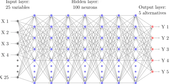
into the utility of alternative 𝑘; and 𝑚 is the total number of layers in a DNN. Figure 2-1 visualizes a DNN architecture with 25 input variables, 5 output alternatives, and 7 hidden layers. The grey nodes represent the input variables; the blue ones repre-sent the hidden layers; and the red ones reprerepre-sent the Softmax activation function. The layer-by-layer architecture in Figure 2-1 reflects the compositional structure of Equation 2.2.
The inputs into the Softmax layers in DNNs can be treated as utilities, the same as those in the classical DCMs. This utility interpretation in DNNs is actually shown by the Lemma 2 in McFadden (1974) [85], which implies that the Softmax activation function is equivalent to a random utility term with Gumbel distribution under the random utility maximization (RUM) framework. Hence DNNs and MNL models are both under the RUM framework, and their difference only resides in the utility
X 1 X 2 X 3 X 4 X 25 Y 1 Y 2 Y 3 Y 4 Y 5 Hidden layer: 100 neurons Input layer:
25 variables Output layer:
5 alternatives
Figure 2-1: A DNN architecture (7 hidden layers * 100 neurons)
specifications. In other words, the inputs into the last Softmax activation function of DNNs can be interpreted as utilities; the outputs from the Softmax activation function are choice probabilities; the transformation before this Softmax function can be seen as a process of specifying utility functions; and the Softmax activation function can be seen as a process of comparing utility values.
DNNs are a much more generic model family than MNL models, and this rela-tionship can be understood from various mathematical perspectives. The universal approximator theorem developed in the 1990s indicates that a neural network with only one hidden layer is asymptotically a universal approximator when the width becomes infinite [30, 59, 58]. Recently this asymptotic perspective leads to a more non-asymptotic question, asking why depth is necessary when a wide and shallow neural network is powerful enough. It has been shown that DNNs can approximate functions with an exponentially smaller number of neurons than a shallow neural network in many settings [29, 109, 103]. In other words, DNNs can be treated as an efficient universal approximator, thus being much more generic than the MNL model, which is a shallow neural network with zero hidden layers. However, from the perspective of statistical learning theory, a more generic model family leads to both smaller approximation errors and large estimation errors. Since the out-of-sample
prediction error equals to the sum of the approximation and estimation errors, DNNs do not necessarily outperform MNL models from a theoretical perspective. The major challenge of DNNs is its large estimation error, which is caused by its extraordinary approximation power. A brief theoretical proof about the large estimation error of DNNs is available in Appendix I. The proof is Appendix I uses Dudley integral and covering argument, which establishes the key intuition about the tradeoff between model complexity and sample size. I also provide a second proof in Appendix II, which focuses on the estimation error of the choice probability functions. The proof in Appendix II uses contraction inequality to generates tighter bound. Appendix II shows how the choice probability functions behave in a non-asymptotic manner. More detailed discussions are available in the recent studies from the field of statis-tical learning theory [136, 139, 42, 92, 10, 77, 9]. For the purpose of this study, it is important to know that the hyperparameter searching is essentially about the control of model complexity, which balances the approximation and estimation errors. This tradeoff between the approximation and estimation errors has a deep foundation in the statistical learning theory discussions.
2.3.2
Computing Economic Information From DNNs
The utility interpretation in DNNs enables us to derive all the economic information traditionally obtained from DCMs. With ˆ𝑉𝑘(𝑥𝑖) denoting the estimated utility of
alternative 𝑘 and ˆ𝑠𝑘(𝑥𝑖) the estimated choice probability function, Table 2.1
summa-rizes the formula of computing the economic information, which is sorted into two categories. Choice probabilities, choice predictions, market share, substitution pat-terns, and social welfare are derived by using functions (either choice probability or utility functions). Probability derivatives, elasticities, MRS, and VOTs are derived from the gradients of choice probability functions. This differentiation is owing to the the different theoretical properties between functions and their gradients 1. The two
categories also relate to different generic methods of interpreting DNNs, as discussed
1The uniform convergence proof is possible for the estimated functions, while it is much harder
in our results section.
Economic Information Formula in DNNs Categories
Choice probability ˆ𝑠𝑘(𝑥𝑖) F
Choice prediction argmax
𝑘
ˆ
𝑠𝑘(𝑥𝑖) F
Market share ∑︀
𝑖ˆ𝑠𝑘(𝑥𝑖) F
Substitution pattern between al-ternatives 𝑘1 and 𝑘2 ˆ 𝑠𝑘1(𝑥𝑖)/ˆ𝑠𝑘2(𝑥𝑖) F Social welfare ∑︀ 𝑖 1 𝛼𝑖log( ∑︀𝐽 𝑗=1𝑒 ^ 𝑉𝑖𝑗) + 𝐶 F
Change of social welfare ∑︀
𝑖 1 𝛼𝑖[︀ log(∑︀ 𝐽 𝑗=1𝑒 ^ 𝑉1 𝑖𝑗) − log(∑︀𝐽 𝑗=1𝑒 ^ 𝑉0 𝑖𝑗)]︀ F
Probability derivative of alterna-tive 𝑘 w.r.t. 𝑥𝑖𝑗
𝜕 ˆ𝑠𝑘(𝑥𝑖)/𝜕𝑥𝑖𝑗 GF
Elasticity of alternative 𝑘 w.r.t. 𝑥𝑖𝑗
𝜕 ˆ𝑠𝑘(𝑥𝑖)/𝜕𝑥𝑖𝑗× 𝑥𝑖𝑗/ˆ𝑠𝑘(𝑥𝑖) GF
Marginal rate of substitution be-tween 𝑥𝑖𝑗1 and 𝑥𝑖𝑗2
−𝜕 ^𝑠𝑘(𝑥𝑖)/𝜕𝑥𝑖𝑗1
𝜕 ^𝑠𝑘(𝑥𝑖)/𝜕𝑥𝑖𝑗2 GF
VOT (𝑥𝑖𝑗1 is time and 𝑥𝑖𝑗2 is
mon-etary value)
−𝜕 ^𝑠𝑘(𝑥𝑖)/𝜕𝑥𝑖𝑗1
𝜕 ^𝑠𝑘(𝑥𝑖)/𝜕𝑥𝑖𝑗2 GF
Table 2.1: Formula to compute economic information from DNNs; F stands for func-tion, GF stands for the gradients of functions.
This process of interpreting economic information from DNNs is significantly dif-ferent from the classical DCMs for the following reasons. In DNNs, the economic information is directly computed by using functions ˆ𝑠𝑘(𝑥𝑖) and ˆ𝑉𝑘(𝑥𝑖), rather than
individual parameters ˆ𝑤. This focus on functions rather than individual parame-ters is inevitable owing to the fact that a simple DNN can easily have thousands of individual parameters. This focus is also consistent with the interpretation studies about DNNs: a large number of recent studies used the function estimators for in-terpretation, while none focused on individual neurons/parameters [88, 55, 5, 110]. In other words, the DNN interpretation can be seen as an end-to-end mechanism without involving the individual parameters as an intermediate process. In addition, the interpretation of DNNs is a prediction-driven process: the economic information is generated in a post-hoc manner after a model is trained to be highly predictive. This prediction-driven interpretation takes advantage of DNNs’ capacity of automatic feature learning, and it is also in contrast to the classical DCMs that rely on
hand-crafted utility functions. This prediction-driven interpretation is based on the belief that “when predictive quality is (consistently) high, some structure must have been found” [90].
2.4
Setup of Experiments
2.4.1
Hyperparameter Training
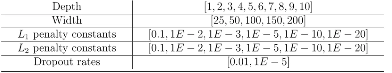
Random searching is used to explore a pre-specified hyperparameter space to identify the DNN hyperparameters with the highest prediction accuracy [16]. The hyperpa-rameter space consists of the architectural hyperpahyperpa-rameters, including the depth and width of DNNs; and the regularization hyperparameters, including 𝐿1 and 𝐿2 penalty
constants, and dropout rates. 100 sets of hyperparameters are randomly generated for comparison. The details of the hyperparameter space is available in Appendix III. Besides the hyperparameters varying across the 100 models, all the DNN models share certain fixed components, including ReLU activation functions in the hidden layers, Softmax activation function in the last layer, Gloret initialization, and Adam optimization, following the standard practice [43, 47]. Formally, the hyperparameter searching is formulated as ˆ 𝑤ℎ = argmin 𝑤ℎ∈{𝑤 (1) ℎ ,𝑤 (2) ℎ ,...,𝑤 (𝑆) ℎ } argmin 𝑤 𝐿(𝑤, 𝑤ℎ) (2.3)
where 𝐿(𝑤, 𝑤ℎ) is the empirical risk function that the DNN training aims to
mini-mize, 𝑤 represents the parameters in a DNN architecture, 𝑤ℎ represents the
hyper-parameter, 𝑤(𝑠)ℎ represents one group of hyperparameters randomly sampled from the hyperparameter space, and ˆ𝑤ℎ is the chosen hyperparameter used for in-depth
eco-nomic interpretation. Besides the random searching, other approaches can be used for hyperparameter training, such as reinforcement learning or Bayesian methods, [122, 152], which are beyond the scope of our study.
2.4.2
Training with Fixed Hyperparameters
After the hyperparameter searching, we examine one group of hyperparameters that lead to the highest prediction accuracy. Then by using the same training set and the fixed group of hyperparameters, we train the DNN models another 100 times to ob-serve whether different trainings lead to differences in choice probability functions and other economic information. Note that the 100 hyperparameter searches introduced in the previous subsection provide evidence about the sensitivity of DNNs to hyperpa-rameters, while the 100 trainings here conditioned on the fixed hyperparameters are designed to demonstrate the model non-identification challenge. Each training seeks to minimize the empirical risk conditioned on the fixed hyperparameters, formulated as following. min 𝑤 𝐿(𝑤, ˆ𝑤ℎ) = min𝑤 − 1 𝑁 𝑁 ∑︁ 𝑖=1 𝑙(𝑦𝑖, 𝑠𝑘(𝑥𝑖; 𝑤, ˆ𝑤ℎ)) + 𝛾||𝑤||𝑝 (2.4)
where 𝑤 represents the parameters; ˆ𝑤ℎ represents the best hyperparameters; 𝑙() is
the loss function, typically the cross-entropy loss function; and 𝑁 is the sample size. 𝛾||𝑤||𝑝 represents 𝐿𝑝 penalty (||𝑤||𝑝 = (∑︀𝑗(𝑤𝑗)𝑝)
1
𝑝), and 𝐿
1 (LASSO) and 𝐿2 (Ridge)
penalties are the two specific cases of 𝐿𝑝 penalties. Note that DNNs have the model
non-identification challenge because the objective function in Equation 2.4 is not globally convex. DNNs have the local irregularity challenge because this optimization over the global prediction risks is insufficient to guarantee the local fidelity. The two issues are caused by related but slightly different reasons.
2.4.3
Dataset
Our experiments use a stated preference (SP) survey conducted in Singapore in July 2017. In total, 2, 073 respondents participated, and each responded to seven choice scenarios that varied in the availability and attributes of the travel mode alternatives. The final dataset with a complete set of alternatives included 8, 418 observations. The choice variable 𝑦 is travel mode choice, including five alternatives: walking,
taking public transit, ride sharing, using an autonomous vehicle, and driving. The explanatory variables include 25 individual-specific and alternative-specific variables, such as income, education, gender, driving costs, and driving time. The dataset is split into the training, validation, and testing sets, with a ratio of 6:2:2, associated with 5,050:1,684:1,684 observations for each. The training set was used for training individual models; the validation set for selecting hyperparameters; the testing set for the final analysis of economic information.
2.5
Experimental Results
This section shows that it is feasible to extract all the economic information from DNNs without involving individual parameters, and that by using the hyperparameter searching and ensemble methods, it is possible to partially mitigate the three problems involved in the DNN interpretation. We will first present the results about prediction accuracy, then the function-based interpretation for choice probabilities, substitution patterns of alternatives, market share, and social welfare, and lastly the gradient-based interpretation for probability derivatives, elasticities, VOT, and heterogeneous preferences. This section focuses on one group of DNN models with five hidden layers and fixed hyperparameters (5L-DNNs), chosen from the hyperparameter searching thanks to their highest prediction accuracy. Note that the 5L-DNNs are chosen based on our hyperparameter searching results using this particular dataset, and this does not at all suggest that this specific architecture is generally the best in the other cases. The 5L-DNNs are compared to two benchmark model groups: (1) the 100 DNN models randomly searched in the pre-specified hyperparameter space (HP-DNNs), and (2) the classical MNL models with linear utility specifications. While it is possible to enrich the linear specifications in the MNL model, it is beyond the scope of this study to explore the different types of MNL models.
2.5.1
Prediction Accuracy of Three Model Groups
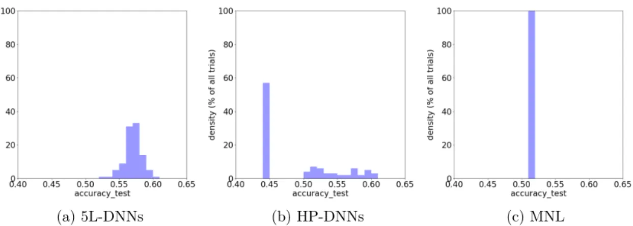
The comparison of the three model groups in Figure 2-2 reveals two findings. First, 5L-DNNs on average outperform the MNL models by about 5-8 percentage points in terms of the prediction accuracy, as shown by the difference between Figure 2-2a and 2-2c. This result that DNNs outperform MNL models is consistent with previous studies [107, 95, 65]. Second, choosing the correct hyperparameter plays a critical role in improving the model performance of DNNs, as shown by the higher prediction accuracy of the 5L-DNNs than the HP-DNNs. With higher predictive performance, the 5L-DNNs are more likely to reveal valuable economic information than the MNL models and the HP-DNNs.
(a) 5L-DNNs (b) HP-DNNs (c) MNL
Figure 2-2: Histograms of the prediction accuracy of three model groups (100 trainings for each model group)
2.5.2
Function-Based Interpretation
Choice Probability Functions
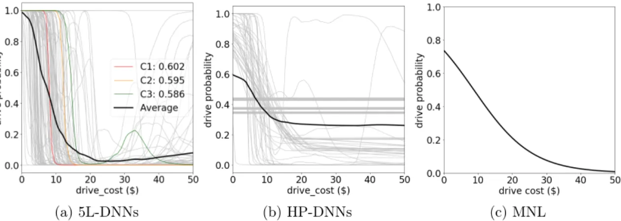
The choice probability functions of the three model groups are visualized in Figure 2-3. Since the inputs of the choice probability functions 𝑠(𝑥) have high dimensions, the 𝑠(𝑥) is visualized by computing the driving probability with varying only the driving cost, holding all the other variables constant at the sample mean. Each light grey curve in Figures 2-3a-2-3b represents one individual training result, and the dark
curve is the ensemble of all 100 models. In Figure 2-3c, only one training result is visualized because the MNL training has no variation.
(a) 5L-DNNs (b) HP-DNNs (c) MNL
Figure 2-3: Driving probability functions with driving costs (100 trainings for each model group)
The results of the 5L-DNNs in Figure 2-3a demonstrate the power of DNNs be-ing able to automatically learn the choice probability functions. From a behavioral perspective, the majority of the choice probability functions in Figure 2-3a are rea-sonable. In comparison to the choice probability functions of MNL (Figure 2-3c), the choice probability functions of the 5L-DNNs are richer and more flexible. The caveat is that the DNN choice probability functions may be too flexible to reflect the true behavioral mechanisms, owing to three theoretical challenges.
First, the large variation of individual models in Figure 2-3b reveal that DNN models are sensitive to the choice of hyperparameters. With different hyperparame-ters, some of HP-DNNs’ choice probability functions are simply flat without revealing any useful information, while others are similar to 5L-DNNs with reasonable patterns. This challenge can be mitigated by hyperparameter searching and model ensemble. For example, the 5L-DNNs can reveal more reasonable economic information than the HP-DNNs because the 5L-DNNs use specific architectural and regularization hy-perparameters, chosen from the results of hyperparameter searching based on their high prediction accuracy. In addition, as shown in Figure 2-3a, the choice probabil-ity function aggregated over models retains more smoothness and monotonicprobabil-ity than individual ones. The average choice probability function predicts that the driving
probability decreases the most when the driving cost increases from about $5 to $20, which is reasonable. Averaging models is an effective way of regularizing models be-cause it reduces the large variance of the models with high complexity, such as DNNs [19].
Second, the large variation of the individual 5L-DNN trainings (Figure 2-3a) reveal the challenge of model non-identification. Given that the 100 trainings are conditioned on the same training data and the same hyperparameters, the variation across the 5L-DNNs in Figure 2-3a is attributable to the model non-identification issue, or more specifically, the optimization difficulties in minimizing the non-convex risk function of DNNs. As DNNs’ risk function is non-convex, different model trainings can converge to very different local minima or saddle points. Whereas these local minima have similar prediction accuracy, it brings difficulties to the model interpretation since the functions learnt from different local minima are different. For example, the three individual training results (C1, C2, and C3) have very similar out-of-sample prediction accuracy (60.2%, 59.5%, and 58.6%); however, their corresponding choice probability functions are very different. In fact, the majority of the 100 individual trainings have quite similarly high prediction accuracy, whereas their choice probability functions differ from each other. On the other side, the choice probability function averaged over the 100 trainings of the 5L-DNNs is more stable than individual ones. In practice, averaging over models is one effective way to provide a stable and reasonable choice probability function for interpretation.
Third, the shapes of the individual curves in Figure 2-3a show the local irregular-ity of the choice probabilirregular-ity functions in certain regions of the input domain. First, some choice probability functions can be sensitive to the small change of input val-ues; for example, the probability of choosing driving in C1 drops from 96.6% to 7.8% as the driving cost increases from $7 to $9, indicating a locally exploding gradient. This phenomenon of exploding gradients is acknowledged in the robust DNN dis-cussions, because exploding gradients render a system vulnerable [111, 110]. Second, many training results present a non-monotonic pattern. For example, C3 represents a counter-intuitive case where the probability of driving starts to increase dramatically
as the driving costs are larger than $25. The local irregularity only exists in a limited region of the input domain: the driving probability becomes increasing when the cost is larger than $25, where the training sample is sparse. As a comparison, the average choice probability function of the 5L-DNNs has only a slight increasing trend when the driving cost is larger than $25, mitigating the local irregularity issue.
Substitution Pattern of Alternatives
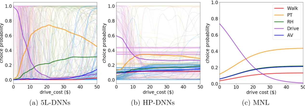
The substitution pattern of the alternatives is of both practical and theoretical im-portance in choice analysis. In practice, researchers need to understand how market shares vary with input variables; in theory, the substitution pattern constitutes the critical difference between multinomial logit, nested logit, and mixed logit models. Figure 2-4 visualizes how the probability functions of the five alternatives vary as the driving cost increases. By visualizing the choice probabilities of all five alternatives, Figure 2-4 is an one-step extension of Figure 2-3.
(a) 5L-DNNs (b) HP-DNNs (c) MNL
Figure 2-4: Substitution patterns of five alternatives with varying driving costs
The substitution pattern of the 5L-DNNs is more flexible than that of the MNL models and more reasonable than that of the HP-DNNs. When the driving cost is smaller than $20, the substitution pattern of the 5L-DNNs aggregated over the 100 models illustrates that the five alternatives are substitute to each other, since the driving probability is decreasing while others are increasing. When the driving cost is larger than $20, the substitution pattern between walking, ridesharing, driving,
and using an AV still reveals the substitute nature. In a choice modeling setting, the alternatives in a choice set are typically substitutes: people are expected to switch from driving to other travel modes, as the driving cost increases. Therefore, the aggregated substitution pattern has mostly reflected the correct relationship of the five alternatives. However, the three theoretical challenges also permeate into the substitution patterns. The large variation in Figure 2-4b illustrates the high sensi-tivity to hyperparameters; the large variation in Figure 2-4a illustrates the model non-identification; and the individual curves in Figure 2-4a reveal the local irregular-ity. Even the model ensemble cannot solve all the problems. When the driving cost is larger than $20, the average substitution pattern of the 5L-DNNs indicate that people are less likely to choose the public transit as the driving cost increases. This phenomenon seems unlikely because driving and public transit are supposed to be substitute to each other. As a comparison, the substitution pattern in Figure 2-4c, although perhaps exceedingly restrictive, reflects the travel mode alternatives being substitute goods. Therefore, DNNs can overall reveal a flexible substitution pattern of alternatives, although the pattern can be counter-intuitive in certain local regions of the input space.
Market Shares
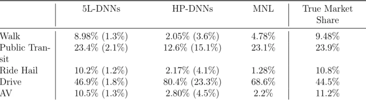
Table 2.2 summarizes the market shares predicted by the three model groups. Each entry represents the average value of the market share over 100 trainings, and the number in the parenthesis is the standard deviation. Whereas the choice probability functions of 5L-DNNs can be unreasonable locally as discussed in section 2.5.2, the aggregated market share of 5L-DNNs are very close to the true market share, and it is more accurate than the HP-DNNs and the MNL models. It appears that the three challenges do not emerge in this discussion about market shares. The local irregularity could be cancelled out owing to the aggregation over the sample; the model non-identification appears less a problem when the market shares across the 5L-DNN trainings are very stable, as shown by the small standard deviations in the parenthesis; and the high sensitivity to hyperparameters is addressed by the selection
of the 5L-DNNs from the hyperparameter searching process, as the market shares of the 5L-DNNs are much more accurate than the HP-DNNs.
5L-DNNs HP-DNNs MNL True Market Share Walk 8.98% (1.3%) 2.05% (3.6%) 4.78% 9.48% Public Tran-sit 23.4% (2.1%) 12.6% (15.1%) 23.1% 23.9% Ride Hail 10.2% (1.2%) 2.17% (4.1%) 1.28% 10.8% Drive 46.9% (1.8%) 80.4% (23.3%) 68.6% 44.5% AV 10.5% (1.3%) 2.80% (4.5%) 2.2% 11.2%
Table 2.2: Market share of five travel modes (testing)
Social Welfare
Since DNNs have an implicit utility interpretation, we can observe how social welfare changes as action variables change the values. To demonstrate this process, we sim-ulate one dollar decrease of the driving cost, and calcsim-ulate the average social welfare change in the 5L-DNNs. We found that the social welfare increases by about $520 in the 5L-DNN models after averaging over all 100 trainings. Interestingly, the magni-tude of this social welfare change ($520) is very intuitive and consistent with the one computed from MNL models, which is $491 dollars. In the process of computing the social welfare change, we used the 𝛼𝑖 averaged across 100 trainings as the individual
𝑖’s marginal value of utility. Without using average 𝛼𝑖, individuals’ marginal value
of utility can take unreasonable values, caused by local irregularity and model non-identification. The problem associated with the individuals’ gradient information will be discussed in details in the following section.
Interpretation Methods
The four subsections above interpret DNNs by using choice probability and util-ity functions. Both are widely used in the generic studies about DNN interpre-tation, although usually referred to by different names. For example, researchers interpret DNNs by identifying the representative observation for each class. The
method is called activation maximization (AM) ˆ𝑥𝑘 = argmax 𝑥
log 𝑃 (𝑦 = 𝑘|𝑥), which maximizes the conditional probability density function with respect to the input 𝑥 [36, 117, 88, 67]. The choice probabilities are also referred to as soft labels, used to distill knowledge by retraining a simple model to fit a complicated DNN [55]. Re-searchers in the computer vision field interpret DNN results by mapping the neurons of the hidden layers to the input space [147] or visualizing the activation maps in the last layer [151]. Since utilities are just the activation maps of the last layer, our interpretation approach is similar to those used in computer vision. In these generic discussions about DNN interpretation, the differentiation between the utility function and the choice probability functions is weak, since their mapping is monotonic and the function properties are similar.
2.5.3
Gradient-Based Interpretation
Gradients of Choice Probability Functions
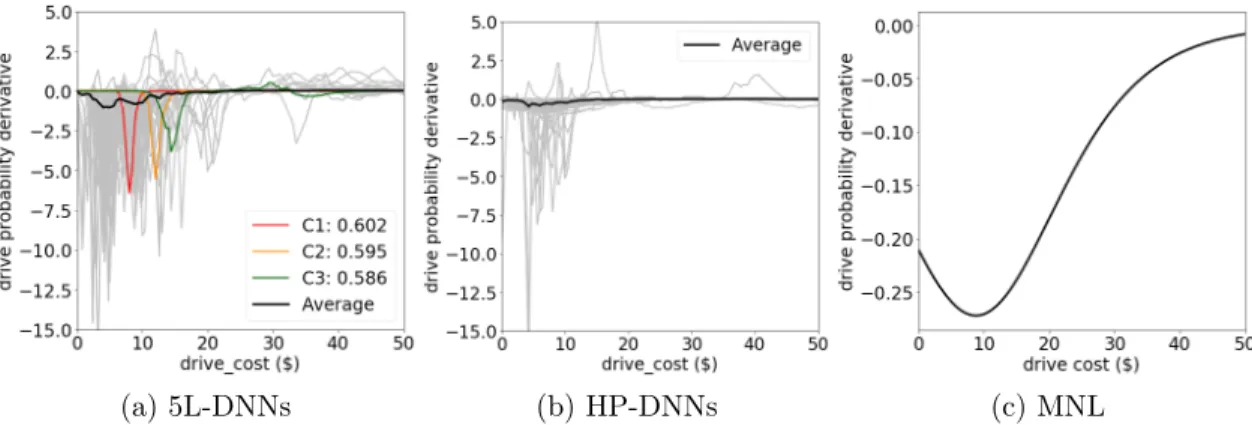
The gradient of choice probability functions offers opportunities to extract more im-portant economic information. Since researchers often seek to understand how to intervene to trigger behavioral changes, the most relevant information is the partial derivative of the choice probability function with respect to a targeting input vari-able. Figure 2-5 visualizes the corresponding probability derivatives of the choice probability functions in Figure 2-3. As shown below, both the strength and the chal-lenges identified in the choice probability functions are retained in the properties of the probability derivatives.
In Figure 2-5a, the majority of the 5L-DNNs, such as the three curves (C1, C2, and C3), take negative values and have inverse bell shapes. This inverse bell shaped curve is intuitive because people are not as sensitive to price changes when price is close to zero or infinity, but are more sensitive when price is close to a certain tipping point. The shapes revealed by 5L-DNNs are similar to the MNL models. The probability derivative of MNL models is 𝜕𝑠(𝑥)/𝜕𝑥 = 𝑠(𝑥)(1−𝑠(𝑥))×(𝜕𝑉 (𝑥)/𝜕𝑥), which is mostly negative and take a very regular inverse bell shape, as shown in Figure 2-5c.
(a) 5L-DNNs (b) HP-DNNs (c) MNL
Figure 2-5: Probability derivatives of choosing driving with varying driving costs
The sensitivity to hyperparameters, the model non-identification, and the local irregularity are also shown in Figure 2-5, similar to the discussions in Figure 2-3. HP-DNNs reveal more unreasonable behavioral patterns than 5L-DNNs, as many of the input gradients are flat on zero, demonstrating the importance of selecting correct hyperparameters. The variation of individual trainings in Figure 2-5a demonstrates the challenge of model non-identification. With fixed training samples and hyper-parameters, the DNN trainings can lead to different training results, thus creating difficulty for researchers to choose a final model for interpretation. The exploding gradients and the non-monotonicity issues, as the two indicators of local irregularity, are also clearly illustrated in the individual trainings in Figure 2-5a. The absolute values of many probability derivatives are of large magnitude; for example, at the peak of the C1 curve, $1 cost increase leads to about 6.5% change in choice probabil-ity2, which is much larger than the MNL models. Similar to the previous discussions,
hyperparameter searching and information aggregation can mitigate these issues.
Elasticities
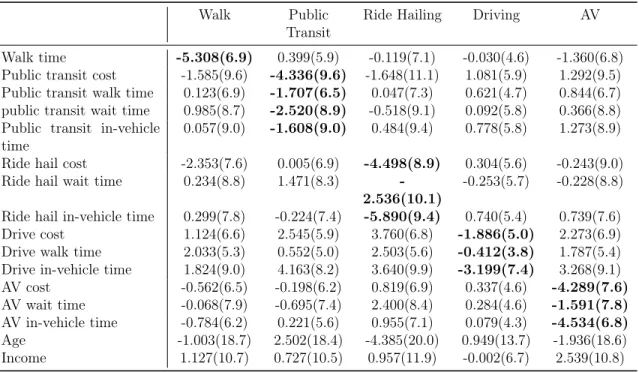
To compare across input variables, researchers often compute elasticities because the elasticities are standardized derivatives. Given that DNNs provide choice probability derivatives, it is straightforward to compute the elasticities from DNNs. Table 2.3
2This 6.5% appears much smaller than the values in Figure 2-3. It is because of the difference
presents the elasticities of travel mode choices with respect to input variables. Each entry represents the average elasticity across the 100 trainings of the 5L-DNNs, and the value in the parenthesis is the standard deviation of the elasticities across the 100 trainings. Unlike a regression table, the standard deviation in Table 2.3 is not caused by the sampling randomness, but by the non-identification of models.
Walk Public
Transit
Ride Hailing Driving AV
Walk time -5.308(6.9) 0.399(5.9) -0.119(7.1) -0.030(4.6) -1.360(6.8) Public transit cost -1.585(9.6) -4.336(9.6) -1.648(11.1) 1.081(5.9) 1.292(9.5) Public transit walk time 0.123(6.9) -1.707(6.5) 0.047(7.3) 0.621(4.7) 0.844(6.7) public transit wait time 0.985(8.7) -2.520(8.9) -0.518(9.1) 0.092(5.8) 0.366(8.8) Public transit in-vehicle
time
0.057(9.0) -1.608(9.0) 0.484(9.4) 0.778(5.8) 1.273(8.9) Ride hail cost -2.353(7.6) 0.005(6.9) -4.498(8.9) 0.304(5.6) -0.243(9.0) Ride hail wait time 0.234(8.8) 1.471(8.3)
-2.536(10.1)
-0.253(5.7) -0.228(8.8) Ride hail in-vehicle time 0.299(7.8) -0.224(7.4) -5.890(9.4) 0.740(5.4) 0.739(7.6) Drive cost 1.124(6.6) 2.545(5.9) 3.760(6.8) -1.886(5.0) 2.273(6.9) Drive walk time 2.033(5.3) 0.552(5.0) 2.503(5.6) -0.412(3.8) 1.787(5.4) Drive in-vehicle time 1.824(9.0) 4.163(8.2) 3.640(9.9) -3.199(7.4) 3.268(9.1) AV cost -0.562(6.5) -0.198(6.2) 0.819(6.9) 0.337(4.6) -4.289(7.6) AV wait time -0.068(7.9) -0.695(7.4) 2.400(8.4) 0.284(4.6) -1.591(7.8) AV in-vehicle time -0.784(6.2) 0.221(5.6) 0.955(7.1) 0.079(4.3) -4.534(6.8) Age -1.003(18.7) 2.502(18.4) -4.385(20.0) 0.949(13.7) -1.936(18.6) Income 1.127(10.7) 0.727(10.5) 0.957(11.9) -0.002(6.7) 2.539(10.8)
Table 2.3: Elasticities of five travel modes with respect to input variables The average elasticities of the 5L-DNNs are reasonable in terms of both the signs and magnitudes. We highlight the elasticities that relate the travel modes to their own alternative-specific variables. These highlighted elasticities are all negative, which is very reasonable since higher travel cost and time should lead to lower probability of adopting the corresponding travel mode. The magnitudes are higher than the typical results from the MNL models. For example, Table 2.3 indicates that 1% increase in public transit cost, walking time, waiting time, and in-vehicle travel time leads to the decrease of 4.3%, 1.7%, 2.5%, and 1.6% probability in using public transit. In addition, the highlighted elasticities are overall of a larger magnitude than others, which is also reasonable since the self-elasticity values are typically larger than cross-elasticity values. Therefore, as the cross-elasticity values are aggregated over the trainings and the sample, these values are quite reasonable.
Model non-identification is revealed here by the large standard deviations of the elasticities. For example, as the walking elasticity regarding walking time is −5.3 on average, its standard deviation is 6.9. This large standard deviation is caused by model non-identification, as every training leads to a different model and a different elasticity. The high sensitivity and the local irregularity issues are not present in the process of computing the average elasticities, because the 5L-DNNs are trained by the same hyperparameter and the local irregularity is partially mitigated by the aggregation over the sample.
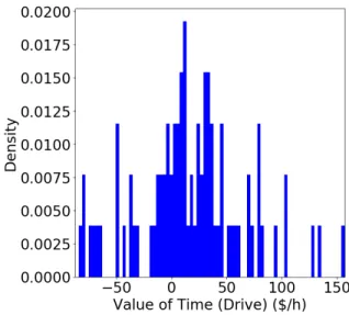
Marginal Rates of Substitution: Values of Time
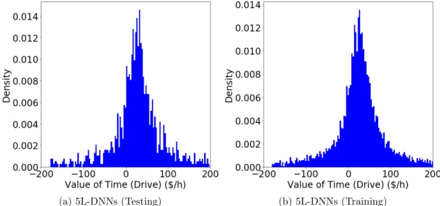
VOT, as one example of MRS, is one of the most important pieces of economic information obtained from choice models, since the monetary gain from time saving is the most prevalent benefit from the improvement of any transportation system. As VOT is computed as the ratio of two parameters in a MNL model, the ratio of two probability derivatives represents the VOT in the DNN setting. Figure 2-6 presents the distribution of the VOTs of the 5L-DNNs. The distribution has a very large dispersion and even some negative values, caused by the model non-identification issue.