Decomposition Techniques for Large-Scale
Optimization in the Supply Chain
by
Lindsay Sanneman
B.S., Massachusetts Institute of Technology (2014)
Submitted to the Department of Mechanical Engineering
in partial fulfillment of the requirements for the degree of
Master of Science in Mechanical Engineering
at the
MASSACHUSETTS INSTITUTE OF TECHNOLOGY
June 2018
c
○ Massachusetts Institute of Technology 2018. All rights reserved.
Author . . . .
Department of Mechanical Engineering
May 25, 2018
Certified by . . . .
Julie A. Shah
Associate Professor of Aeronautics and Astronautics
Thesis Supervisor
Certified by . . . .
John J. Leonard
Samuel C. Collins Professor of Mechanical and Ocean Engineering
Thesis Supervisor
Accepted by . . . .
Rohan Abeyaratne
Chairman, Department Committee on Graduate Students
Decomposition Techniques for Large-Scale Optimization in
the Supply Chain
by
Lindsay Sanneman
Submitted to the Department of Mechanical Engineering on May 25, 2018, in partial fulfillment of the
requirements for the degree of
Master of Science in Mechanical Engineering
Abstract
Integrated supply chain models provide an opportunity to optimize costs and produc-tion times in the supply chain while taking into consideraproduc-tion the many steps in the production and delivery process and the many constraints on time, shared resources, and throughput capabilities. In this work, mixed integer linear programming (MILP) models are developed to describe the manufacturing plant, consolidation transport, and distribution center components of the supply chain. Initial optimization results are obtained for each of these models. Additionally, an integrated model including a single plant, multiple consolidation transport vehicles, and a single distribution cen-ter is formulated and initial results are obtained. All models are implemented and optimized for their given objectives using a standard MILP solver.
Initial optimization results suggest that it is intractable to solve problems of rel-evant scale using standard MILP solvers. The natural hierarchical structure in the supply chain problem lends itself well to application of decomposition techniques in-tended to speed up solution time. Exact techniques, such as Benders decomposition, are explored as a baseline. Classical Benders decomposition is applied to the man-ufacturing plant model, and results indicate that Benders decomposition on its own will not improve solve times for the manufacturing plant problem and instead leads to longer solve times for the problems that are solved. This is likely due to the large number of discrete variables in manufacturing plant model.
To improve upon solve times for the manufacturing plant model, an approximate decomposition technique is developed, applied to the plant model, and evaluated. The approximate algorithm developed in this work decomposes the problem into a three-level hierarchical structure and integrates a heuristic approach at two of the three levels in order to solve abstracted versions of the larger problem and guide to-wards high-quality solutions. Results indicate that the approximate technique solves problems faster than those solved by the standard MILP solver and all solutions are within approximately 20% of the true optimal solutions. Additionally, the approx-imate technique can solve problems twice the size of those solved by the standard MILP solver within a one hour timeframe.
Thesis Supervisor: Julie A. Shah
Title: Associate Professor of Aeronautics and Astronautics Thesis Supervisor: John J. Leonard
Acknowledgments
I would first like to thank my advisor, Professor Julie Shah, for all she has done to support me through my last few years of research. Her support and caring really go above and beyond, and her positivity and encouragement have helped foster in me an excitement about research and graduate school. Her encouraging words have made such a difference to me, especially during some of the harder times. She has taught me so much, and I feel very lucky to have her as my advisor.
I would also like to thank Steelcase for funding my research and particularly Jennifer Tyler and Ed Vanderbilt for their guidance as I worked towards the Masters thesis.
My labmates in IRG have made the last few years some of the best years of my life. Everyone is so intelligent and supportive, and each person has each contributed to this thesis or to the other things I have done in graduate school in some way. I enjoy laughing with all of you and the coffee runs we take. You are all treasured friends of mine and make me excited to come into lab every morning.
I would also like to thank Professor Daniela Rus for her mentorship and guidance in the year before I began graduate school. I learned a lot about how to be an effective researcher from her and from my time in the Distributed Robotics Lab. I also learned a lot and laughed a lot with my DRL labmates, Joseph DelPreto, Ankur Mehta, and Robert Katzschmann, and I am grateful to them for all that they’ve taught me and all the fun we’ve had.
Joining the Lutheran Episcopal Ministry at the beginning of grad school was one of the happiest accidents of my life. I enjoy the conversations and deep questions we share in LEM and the humility with which everyone approaches faith. I would like to thank all of my LEM friends for their thoughtfulness and compassion. I very much look forward to taking a break with all of them every Wednesday, and I learn so much from each one of them. I especially want to thank the chaplains, Kari Jo Verhulst and Thea Keith-Lucas. They have been listening ears and pillars of support for me through my first years of grad school, and I cannot thank them enough for
their kindness and caring.
I would also like to thank everyone at the University Lutheran Church. I have truly found a home at UniLu, and I am so grateful to be surrounded by such a thoughtful group of people who care deeply about social justice issues and the wellbeing of all people. Each person at UniLu inspires me to strive to love others more and to love others in new ways every day.
I would also like to thank our Sanctuary guests at UniLu, a mom and her two wondeful daughters. The mom has taught me more about courage and strength than she knows, and the younger two bring me such joy every Friday with their energy, smiles, and playful spirits. I have been so blessed to watch the younger ones learn and grow over the last year, and I feel very lucky to know all three.
I would also like to thank all of the MIT pole vaulters past and present. They all have brought me many laughs over the years, and cheering each of them on through ups and downs has been one of the great joys of my time in graduate school so far. You guys are amazing, and I know each and every one of you will accomplish big things. Never forget your worth and how incredibly capable you are!
I especially want to thank Kathleen Brandes, who has been there for me through both some of the more difficult parts of grad school (including the qualification exams) and the fun parts. Her care and compassion and our shared sense of humor keep me going and inspire me every day.
I also want to thank wonderful, quirky, and witty 1W in East Campus. They brighten my days and really make our hall feel like a family. And beyond that, they have supported me and Patrick and taught us so much, even as we hope to support and teach them.
And I would like to thank the EC house team members (especially Rob Miller and Sandy Alexandre), who are all immensely passionate about student support and care so much about the wellbeing of our wonderful community (sorry,Yonadav!). Each and every person’s care for the students goes well beyond the call and is part of what I love about MIT. I aspire to be a little more like each of you every day.
much. She was there on my first day as a member of IRG and has been there through all the ups and downs of graduate school since. She has always been a cheerleader in my life, and I am so lucky to call her my friend.
I would also like to thank all of my other friends, including Katherine Evans, Rachel Luo, the Sharpes, the Coles, the Balls, and everyone from Arizona. Katherine, especially has been a dear friend of mine and has picked me up when I’ve been down and has been the source of many adventures over the years. And Rachel has been a great travel buddy and friend from our very first days at MIT. I also want to thank all of my other mentors over the years, including teachers from Rancho Solano and Dan, Pam, and Vasko from Arizona Sunrays.
Finally, I would like to thank my family, who has always loved and supported me. My parents have done so much for me and have always made a point to be there for me for both the big moments in life and the smaller ones. I would also like to thank Elise for her love and all of my grandparents for their love. They have all been so invested in me throughout my life, and they mean the world to me. I would like to thank my Grandma Betty in a special way. She taught me nearly everything I know about love, and I am forever grateful for all the time I had to learn from her. One of my favorite memories is being with her during my undergraduate gradution, and she will be greatly missed at this one. And I would lastly like to thank Patrick who has loved and supported me throughout grad school and who has taught me so much about supporting others. I would not have made it this far without him.
Contents
1 Introduction 17
1.1 Motivation . . . 18
1.2 Supply Chain Modeling . . . 18
1.3 Exact Techniques . . . 20
1.4 Approximate Techniques . . . 21
1.5 Conclusions and Future Work . . . 22
2 Supply Chain Modeling 25 2.1 Related Work . . . 26
2.2 Manufacturing Plant . . . 28
2.2.1 Manufacturing Plant Inputs, Outputs, Objective, and Constraints 29 2.2.2 Manufacturing Plant MILP Formulation . . . 30
2.2.3 Manufacturing Plant Results and Discussion . . . 33
2.2.4 Limitations of the Manufacturing Plant Model . . . 35
2.3 Consolidation Transport . . . 36
2.3.1 Consolidation Transport Inputs, Outputs, Objective, and Con-straints . . . 37
2.3.2 Consolidation Transport MILP Formulation . . . 37
2.3.3 Consolidation Transport Results and Discussion . . . 39
2.3.4 Limitations of the Consolidation Transport Model . . . 40
2.4 Distribution Center . . . 41
2.4.1 Distribution Center Inputs, Outputs, Objective, and Constraints 42 2.4.2 Distribution Center MILP Formulation . . . 43
2.4.3 Distribution Center Results and Discussion . . . 45
2.4.4 Limitations of the Distribution Center Model . . . 46
2.5 Integrated Model . . . 47
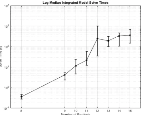
2.5.1 Integrated Model Results and Discussion . . . 48
2.5.2 Limitations of the Integrated Model . . . 50
2.6 Future Modeling and Integration Work . . . 51
3 Exact Techniques 53 3.1 Related Work . . . 53
3.2 Benders Decomposition . . . 55
3.2.1 Overview . . . 55
3.2.2 Benders Decomposition Applied to the Manufacturing Plant Problem . . . 60
3.3 Results and Discussion . . . 65
3.4 Future Work . . . 67
4 Approximate Techniques 69 4.1 Related Work . . . 69
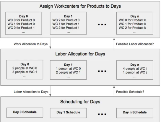
4.2 Hierarchical Approximate Technique . . . 73
4.2.1 Overview . . . 73
4.2.2 Top Level: Work Allocation to Days . . . 76
4.2.3 Middle Level: Labor Allocation to Workcenters . . . 78
4.2.4 Bottom Level: Scheduling . . . 80
4.2.5 Incompleteness of Approximate Technique . . . 84
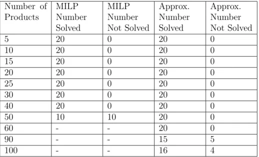
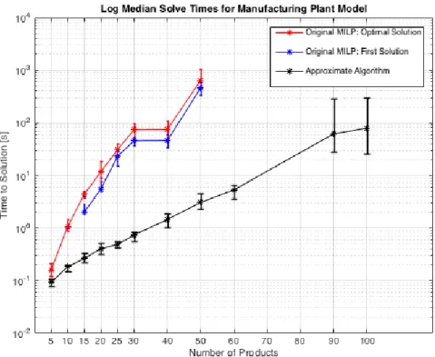
4.3 Results and Discussion . . . 84
4.4 Future Work . . . 89
5 Conclusion 91 5.1 Summary of Results . . . 91
A Benders Decomposition Formulations for the Manufacturing Plant
Problem 97
A.1 Benders Optimality Cut Formulation . . . 98 A.2 Feasibility Cut Formulation . . . 99 A.3 Full Formulation of Benders Dual Subproblem . . . 100
List of Figures
1-1 Supply Chain Integrated Model Layout . . . 20
2-1 Log Median Manufacturing Plant Model Runtimes for Three Workcen-ters, 10 Day Time Horizon . . . 36
2-2 Log Median Consolidation Transport Model Runtimes . . . 41
2-3 Log Median Distibution Center Model Runtimes . . . 46
2-4 Log Median Integrated Model Model Runtimes . . . 50
4-1 Approximate Algorithm Hierarchy . . . 76 4-2 Log Median Solve Times for Original MILP and Approximate Algorithm 88
List of Tables
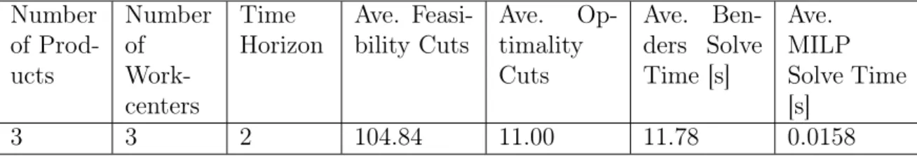
3.1 Feasibility Cuts, Optimality Cuts, and Solve Times for Two Days, Three Products . . . 66 4.1 Number of Problems Solved in under One Hour for Varying Problem
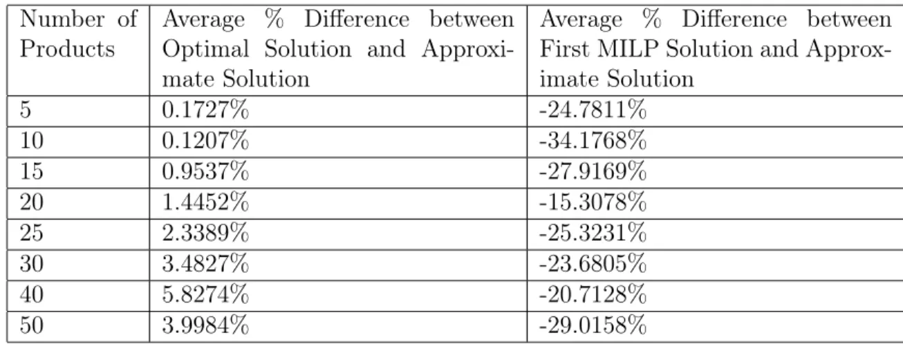
Sizes . . . 86 4.2 Average Percent Differences between Approximate Solutions and MILP
Solutions . . . 89 4.3 Percentage of Problems in which Initial MILP Solution is Better than
Chapter 1
Introduction
The supply chain is a rich domain involving many different processes and handoffs that must integrate smoothly in order to take products from a material acquisition stage all the way to delivery to the final customer. Due to the complex nature of this problem and the costs associated with lost time in supply chain processes, it is of value to model and optimize these processes such that resources are used in a cost effective manner and deadlines are met. There are many different types of supply chains, and each supply chain might involve a number of stages. In this thesis, the specific case of a furniture manufacturing supply chain is explored, and models and assumptions are based on discussions with Steelcase, a furniture manufacturing company, about its supply chain processes. Three primary processes in the Steelcase supply chain include product manufacturing, distribution center operations, and transportation planning, and these three processes are the focus of this thesis. Models developed for supply chain components must balance both sufficient generality to describe the structure of the possibly-varying aspects of the supply chain processes as well as sufficient specificity to optimize the processes well. It is also important to consider the transitions between the different steps in the supply chain and to incorporate information about how a product will move downstream when scheduling upstream processes. To this end, the main contributions of this thesis include the following:
consolidation transport and an integrated model that incorporates the processes involved in all three.
∙ The application of an exact decomposition technique, Benders decomposition, to the manufacturing plant model.
∙ The development of a hierarchical approximate algorithm and its application to the manufacturing plant problem.
1.1
Motivation
While researchers and companies have previously developed models for the different supply chain components, typically when each step in the process is optimized in-dependently, it is likely that the overall flow through all steps in the supply chain process for any given product is suboptimal. Because of this, integrating the opti-mization of the numerous steps in the supply chain process into a single model is of interest. However, in the case of the furniture manufacturing supply chain explored in this work, thousands of products need to be scheduled through dozens of processes each week, so an integrated model will become very large for real-world-sized prob-lems. As orders come in and need to be scheduled through all processes, optimization techniques need to be able to optimize schedules and resources quickly enough to keep up with demand and operations, likely within in sub-hour timeframes. Instead of searching for exact optimal solutions, approximate techniques could provide a way to solve such problems more quickly while outputting near-optimal solutions.
1.2
Supply Chain Modeling
Chapter 2 details the models that were developed for each component of the sup-ply chain as part of this work and the assumptions that were made in developing these models. All components were developed as Mixed Integer Linear Program-ming (MILP) models, and the Gurobi optimizer for Java was used to solve them
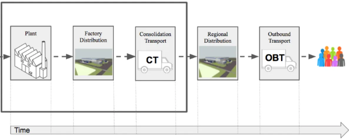
[16]. Three separate models were developed, including a manufacturing plant model, a consolidation transport model, and a distribution center model. The manufactur-ing plant model considers labor allocations to workcenters along the manufacturmanufactur-ing line and scheduling of products through the required workcenters. The consolidation transport model is a vehicle packing and scheduling problem, taking into considera-tion vehicle capacity constraints and scheduled deadlines for products that are packed onto the vehicles. Finally, the distribution center model considers capacity constraints over time as products move into and out of the distribution centers. Chapter 2 also details an integrated model that was developed. The integrated model includes one manufacturing plant, one distribution center, and one set of consolidation transport vehicles. Figure 1-1 shows how products flow through each of the supply chain com-ponents in the case of the Steelcase supply chain: from the manufacturing plant to a factory distribution center, then onto consolidation transport vehicles in order to be shipped to a regional distribution center, and then finally onto outbound transport vehicles for delivery to the final customer. The boxed components are components that are incorporated into the integrated model. Both the regional distribution center and factory distribution center are modeled in the same way, and development and integration of an outbound transportation model is left as future work. In chapter 2, specifics of assumptions made for each of the models are given along with details about experiments run to test each model. Results for the three separate supply chain component models and the integrated model are included. The primary findings in chapter 2 include the following:
∙ The Gurobi optimizer was only able to solve problems an order of magnitude smaller than those those of relevant size in the real-world supply chain for the manufacturing plant MILP model, the distribution center MILP model, and the integrated model. Larger consolidation transport MILP problems were solved using Gurobi, but the problems that were solved were still not as large as those that are dealt with in the real-world supply chain.
Figure 1-1: Supply Chain Integrated Model Layout
tested in chapter 2 is likely limited by the increase in number of decision vari-ables and constraints with the increase in problem size.
1.3
Exact Techniques
While it is convenient to model different components of the supply chain in the MILP framework, solving these problems is in general NP-hard (Bertsimas and Weisman-tel [5]). A number of exact decomposition techniques have been developed to solve problems with the MILP structure more quickly by exploiting their decomposable structures. In particular, MILP problems can be split into a master problem and one or multiple subproblems with all binary- and integer-valued variables in the mas-ter problem and all continuous decision variables in the subproblem(s). Chapmas-ter 3 discusses such techniques in more detail, and one technique in particular, Benders decomposition, is detailed further and applied to the manufacturing plant problem. Implementation details for Benders decomposition applied to the manufacturing plant problem and corresponding results are given. The primary findings in chapter 3 in-clude the following:
∙ It was not possible to solve even the smallest problems that were solved with the manufacturing plant MILP model in chapter 2 with the Benders decompo-sition implementation for the manufacturing plant problem. This suggests that
Benders decomposition will not decrease the solution time as will be necessary for solving real-world scale problems and instead increases solution time.
∙ The primary bottleneck in solving the manufacturing plant problem using Ben-ders decomposition is that in general, many more feasibility cuts are added than optimality cuts, causing slow convergence. This is likely a byproduct of a relatively large number of binary- and integer-valued decision variables as com-pared with the number of continuous decision variables in the problem. Specific details of the feasibility and optimality cuts within the Benders decomposition framework are provided in chapter 2.
1.4
Approximate Techniques
Though exact decomposition techniques have been shown to provide runtime im-provements for certain types of models with a decomposable structure, in general they are not sufficient to provide the necessary improvements in runtimes to solve re-alistic supply chain-sized problems in relevant timeframes. In chapter 4, approximate techniques are explored as a way of achieving high quality solutions in less time than exact techniques take to find the true optimal solution. An approximate technique is developed and is applied to the manufacturing plant problem. Results are given. The primary findings in chapter 4 include the following:
∙ The approximate technique solved manufacturing plant problems faster than the Gurobi optimizer solved the corresponding MILP formulations in all cases in which both techniques solved the problem before a one hour timeout.
∙ On average, the approximate technique arrived at its final solution before the Gurobi optimizer found its first solution to the MILP formulation.
∙ The approximate technique could solve problems twice as large as those solved with the Gurobi MILP formulation within a one hour time horizon.
∙ Due to a bottleneck caused by the lowest level MILP in the approximate tech-nique, the size of problem that can be solved using the approximate technique will be limited.
∙ Solution quality for the approximate technique declined as problem size in-creased, although all approximate solutions were within 20.35% of the solution outputted by Gurobi in cases in which both techniques solved the problem.
1.5
Conclusions and Future Work
Chapter 5 details a summary of the results from this thesis and future work as it re-lates to the results. MILP models were developed for three components of the supply chain including the manufacturing plant, consolidation transport, and the distribution center, and an integrated model was also created and evaluated. Solving these mod-els using the Gurobi optimizer suggested that for real-world-sized problems involving thousands of products to be scheduled in sub-hour timeframes, alternate techniques will be necessary. An exact decomposition technique, Benders decomposition, was applied to the manufacturing plant problem to serve as a baseline for exploration of decomposition techniques for problems like the ones developed in this work. Due to the structure of the manufacturing plant problem, Benders decomposition showed no improvement over solving the original MILP formulation using Gurobi. Explor-ing modified exact techniques, such as Benders decomposition with callbacks, could improve computational performance on problems with a large number of binary and integer decision variables, like the manufacturing plant model developed in this work. An approximate decomposition technique was developed and applied to the manu-facturing plant problem, and computational improvements were achieved using this technique as compared with solving the original MILP formulation using Gurobi. A bottleneck remains in the lowest level scheduling problem of the approximate tech-nique, since this is modeled as a MILP. Exploration of ways to reduce the impact of this bottleneck and thereby solve larger problems is left as future work. Some interesting additional future directions include:
∙ The expansion of the integrated model to account for additional complexity in the supply chain and other supply chain components that are not modeled in this thesis.
∙ Consideration of stochasticity in the supply chain models.
∙ An exhaustive study of different frameworks that could be used to model the supply chain problem.
∙ Application of machine learning techniques to better model different aspects of the supply chain and to allow models to generalize better.
Chapter 2
Supply Chain Modeling
The model of the supply chain proposed in this work includes three generalized sup-ply chain components and an integrated model incorporating the three components and the interactions between them. These models were developed through discussions with an industry partner to ensure that they represent a real world problem well. The three components included in modeling efforts are the manufacturing plant, consol-idation transport, and the distribution center. An outbound transport and delivery model will be added and integrated as part of future work.
Figure 1-1 in chapter 1 shows the layout of the supply chain components used for the integrated model in this work. The ordering of the components in the figure and implemented in the integrated model is used to demonstrate how the supply chain components developed as part of this work can be integrated to optimize over a larger portion of the supply chain as opposed to individual pieces. However, each component presented here functions as an individual piece that can be integrated into supply chain models according to many different configurations.
In this supply chain layout, orders are first received and scheduled for production at a manufacturing plant. After they are produced at the manufacturing plant, they move to a distribution center at the manufacturing plant where they are collected to be assigned to vehicles, called consolidation transport vehicles, that transport them to regional distribution centers. At regional distribution centers, products are collected from various manufacturing plants such that they can be shipped to the
final customer destinations in a single shipment. Finally, products are grouped onto outbound transport vehicles at the regional distribution center, and the outbound transport vehicles are routed to customer destinations. Each of the implemented model components is detailed further in the following sections, and the outbound transport component will developed as future work.
Each model was formulated as a mixed integer linear program (MILP) since the MILP framework lends itself well to a wealth of decomposition techniques that can be used to solve problems more quickly. All MILP models are formulated and solved using Gurobi for Java [16]. Some of the decomposition techniques that can be applied to MILP models are explored further in chapters 3 and 4.
2.1
Related Work
The supply chain with its various components has been modeled in the literature using the MILP framework as well as other frameworks, such as constraint program-ming (CP), and the focuses of the different models that have been developed vary. For example, Castro and Grossmann [9] propose a multistage, multi-product model of the manufacturing plant and formulate the problem as a continuous-time MILP. This model accounts for multiple workcenters and multiple products, but it assumes that all workcenters are required for all products, so it does not cover cases in which products only require a subset of the workcenters. The model developed is compared with a discrete-time MILP formulation and a CP formulation for three different ob-jectives including minimizing cost, minimizing earliness, and minimizing makespan. The CP formulation is shown to perform well for the makespan minimization problem, the discrete-time formulation is shown is perform well for the earliness minimization problem, and the continuous-time formulation performs best with the cost minimiza-tion problem. The model they propose does not consider multi-objective problems. Floudas and Lin [14] perform a review of both discrete-time and continuous-time MILP models describing scheduling of manufacturing plant processes. They note that discrete-time models can be limited in the fact that many decisions variables
are necessary to achieve required accuracy for some production scheduling problems, and continuous-time approaches can reduce the number of required decision variables by employing event variables for things like start times and end times of production processes.
In addition to manufacturing plant models, other components of the supply chain have also been modeled using the MILP framework. For instance, Fanti, Stecco, and Ukovich [13] propose two MILP models to describe distribution center operations with the objective of minimizing operation time. While the models they propose account for unloading and loading processes at the distribution center, constraint capacities are eliminated in order to make the problems tractable to solve, and information about facility volumetric capacity is lost. Additionally, Maheut and Garcia-Sabater [20] model a transportation planning problem with the objective of minimizing vehicle usage using the MILP framework. In their model, vehicles are loaded while accounting for stock levels over time. However, they do not consider the flow of specific products through the supply chain and instead consider only inventories. In the motivating supply chain example considered in this work, specific products need to be tracked and scheduled through manufacturing processes, distribution centers, and transportation processes.
Integrated supply chain models have also been proposed in the literature. You, Grossmann, and Wassick [30] formulate a MILP model for simultaneous capacity, production, and distribution planning for a multi-site system and explore bi-level and Lagrangian decomposition techniques for solving the large-scale MILP models. Their model considers production trains at multiple production facilities and transit to dis-tribution centers in multiple locations downstream. It does not consider specifics of vehicle packing and routing between locations and additionally does not track individ-ual products through the supply chain, but rather considers high level capacities and flows. Application of bi-level and Lagrangian decomposition techniques showed solve time improvements for the examples given, and the bi-level technique showed greater improvement than the Lagrangian decomposition technique in all cases in which im-provements were achieved. Sitek and Wikarek [25] propose a model integrating
man-ufacturing plants, distributors, and customers and formulate it as a hybrid CP/MILP model. In their model, details of production processes at the manufacturing plant are abstracted away. They solve a pure MILP formulation of the problem in addition to the hybrid model both with and without constraint propagation. The greatest improvement over the pure MILP formulation is achieved by the hybrid model in-corporating constraint propagation. Other integrated supply chain models explore other aspects of the supply chain such as retailers, suppliers, and transportation con-siderations (Masoud [21], Pujari [22], Sitek and Wikarek [26]). While a wealth of models have been developed describing different components of the supply chain and the integrated supply chain, many of these models abstract away details that could contribute to overall more optimal end-to-end scheduling of production, transporta-tion, and distribution of products through the supply chain. The work in this thesis aims to model and integrate some of these details, particularly at the manufacturing plant level. Since the integrated models that have been developed in prior literature have many decision variables and constraints for the real-world-sized problems they aim to optimize, decomposition techniques have been explored for solving a number of the models that have been developed. A second goal of the work in this thesis is to further analyze decomposition techniques that could be used to solve real-world-sized problems.
2.2
Manufacturing Plant
The manufacturing plant problem formulated in this work is a labor allocation and scheduling problem. Each manufacturing plant has a set of workcenters that can each accommodate a minimum and maximum amount of labor. A workcenter is a single station in the assembly line that performs one unit of the total required work for the manufacturing process. Different amounts of labor correspond to different cycle times for production at a given workcenter. A cycle time is the amount of time a workcenter takes to perform one unit of work on one product. Items that need to be produced at each manufacturing plant might require a subset or all of
the workcenters at the plant for production. Precedence constraints exist between workcenters, and for all products, workcenters are visited in the same order, but not all workcenters are necessarily required for all products. The manufacturing plant model assumes deterministic cycle times for given labor allocations, that there is no absolute maximum on the available labor across the problem time horizon, and that workcenters accommodate production of one product at a time. It is also assumed that each day in the time horizon has a constant length in hours, and all work can be scheduled at any time within that number of hours for a given day.
2.2.1
Manufacturing Plant Inputs, Outputs, Objective, and
Constraints
The inputs of the manufacturing plant problem are the cycle times corresponding to the different labor allocations at each workcenter, labor allocation minimums and maximums for each workcenter, the problem time horizon, the list of products that need to be produced and their required workcenters, and each product’s deadline. The outputs of the manufacturing plant problem are the labor allocation to the workcen-ters across the problem time horizon and production schedule for each product being processed at the manufacturing plant.
The objective of the manufacturing plant problem is to minimize the total labor requirement, thereby minimizing cost, and simultaneously to schedule the production of each product as close to its deadline as possible. This will minimize the time it sits in the distribution center at the manufacturing plant to prevent overcrowding of the space. Currently, each term in the multi-objective problem is weighted evenly.
At a high level, the constraints in the manufacturing plant problem include the following:
1. The labor assigned to each workcenter for each day falls between the minimum and maximum for that workcenter.
3. Each product is only being produced at one workcenter at a time.
4. Each product should only be scheduled at each of its required workcenters once in the total time horizon.
5. Each workcenter should completely finish a unit of work before the end of the day (non-preemption).
2.2.2
Manufacturing Plant MILP Formulation
The formal manufacturing plant MILP formulation is as follows:
𝑚𝑖𝑛 ∑︁ 𝑖∈𝐼,𝑗∈𝐽,𝑙∈𝐿 𝑌𝑖𝑗𝑙+ ∑︁ 𝑘∈𝐾 𝑄𝑘 (2.1) 𝐴𝑖𝑗 ≤ 𝑚𝑎𝑥𝐿𝑎𝑏𝑜𝑟𝑗 ∀ 𝑖 ∈ 𝐼, 𝑗 ∈ 𝐽 (2.2) 𝐴𝑖𝑗 ≥ 𝑚𝑖𝑛𝐿𝑎𝑏𝑜𝑟𝑗 ∀ 𝑖 ∈ 𝐼, 𝑗 ∈ 𝐽 (2.3) 𝐴𝑖𝑗 = ∑︁ 𝑙∈𝐿 𝑙 · 𝑌𝑖𝑗𝑙 ∀ 𝑖 ∈ 𝐼, 𝑗 ∈ 𝐽 (2.4) ∑︁ 𝑙∈𝐿 𝑌𝑖𝑗𝑙 = 1.0 ∀ 𝑖 ∈ 𝐼, 𝑗 ∈ 𝐽 (2.5) 𝐾𝑖𝑗𝑘𝑙 ≤ 𝑌𝑖𝑗𝑙 ∀ 𝑖 ∈ 𝐼, 𝑗 ∈ 𝐽, 𝑘 ∈ 𝐾, 𝑙 ∈ 𝐿 (2.6) 𝐾𝑖𝑗𝑘𝑙 ≤ 𝐹𝑖𝑗𝑘 ∀ 𝑖 ∈ 𝐼, 𝑗 ∈ 𝐽, 𝑘 ∈ 𝐾, 𝑙 ∈ 𝐿 (2.7) 𝐾𝑖𝑗𝑘𝑙≥ 𝑌𝑖𝑗𝑙+ 𝐹𝑖𝑗𝑘− 1 ∀ 𝑖 ∈ 𝐼, 𝑗 ∈ 𝐽, 𝑘 ∈ 𝐾, 𝑙 ∈ 𝐿 (2.8) 𝑆𝑖𝑗𝑘+ ∑︁ 𝑙∈𝐿 𝑐𝑦𝑐𝑙𝑒𝑇 𝑖𝑚𝑒𝑠𝑗𝑙· 𝑤𝑜𝑟𝑘𝑐𝑒𝑛𝑡𝑒𝑟𝑠𝑘𝑗 · 𝐾𝑖𝑗𝑘𝑙 ≤ 𝑆𝑖,𝑗+1,𝑘 ∀ 𝑖 ∈ 𝐼, 𝑗 ∈ 𝐽, 𝑘 ∈ 𝐾 (2.9)
𝑆𝑖𝑗𝑘+ ∑︁ 𝑙∈𝐿 𝑐𝑦𝑐𝑙𝑒𝑇 𝑖𝑚𝑒𝑠𝑗𝑙· 𝑤𝑜𝑟𝑘𝑐𝑒𝑛𝑡𝑒𝑟𝑠𝑘𝑗 · 𝐾𝑖𝑗𝑘𝑙 ≥ 𝑆𝑖,𝑗+1,𝑘− 𝑀1· 𝑤𝑜𝑟𝑘𝑐𝑒𝑛𝑡𝑒𝑟𝑠𝑘,𝑗+1 ∀ 𝑖 ∈ 𝐼, 𝑗 ∈ 𝐽, 𝑘 ∈ 𝐾 (2.10) ∑︁ 𝑖∈𝐼 𝐹𝑖𝑗𝑘= 1.0 ∀ 𝑖 ∈ 𝐼, 𝑗 ∈ 𝐽, 𝑘 ∈ 𝐾 (2.11) 𝐺𝑖𝑗𝑘 ≤ ℎ𝑜𝑢𝑟𝑠𝑃 𝑒𝑟𝑆ℎ𝑖𝑓 𝑡 · 𝐹𝑖𝑗𝑘 ∀ 𝑖 ∈ 𝐼, 𝑗 ∈ 𝐽, 𝑙𝑘 ∈ 𝐾 (2.12) 𝐺𝑖𝑗𝑘 ≤ 𝑆𝑖𝑗𝑘 ∀ 𝑖 ∈ 𝐼, 𝑗 ∈ 𝐽, 𝑘 ∈ 𝐾 (2.13) ℎ𝑜𝑢𝑟𝑠𝑃 𝑒𝑟𝑆ℎ𝑖𝑓 𝑡·𝐹𝑖𝑗𝑘+𝑆𝑖𝑗𝑘 ≤ 𝐺𝑖𝑗𝑘+ℎ𝑜𝑢𝑟𝑠𝑃 𝑒𝑟𝑆ℎ𝑖𝑓 𝑡 ∀ 𝑖 ∈ 𝐼, 𝑗 ∈ 𝐽, 𝑘 ∈ 𝐾 (2.14) 𝐺𝑖𝑗𝑘 ≥ 0 ∀ 𝑖 ∈ 𝐼, 𝑗 ∈ 𝐽, 𝑘 ∈ 𝐾 (2.15) ∑︁ 𝑙∈𝐿 𝑐𝑦𝑐𝑙𝑒𝑇 𝑖𝑚𝑒𝑠𝑗𝑙· 𝑤𝑜𝑟𝑘𝑐𝑒𝑛𝑡𝑒𝑟𝑠𝑘𝑗· 𝑌𝑖𝑗𝑙+ 𝑤𝑜𝑟𝑘𝑐𝑒𝑛𝑡𝑒𝑟𝑠𝑘𝑗· 𝐺𝑖𝑗𝑘 ≤ ℎ𝑜𝑢𝑟𝑠𝑃 𝑒𝑟𝑆ℎ𝑖𝑓 𝑡 ∀ 𝑖 ∈ 𝐼, 𝑗 ∈ 𝐽, 𝑘 ∈ 𝐾 (2.16) 𝑆𝑖𝑗𝑘+ 𝐿𝑖𝑗𝑘𝑚 ≥ 𝑆𝑖𝑗𝑚 ∀ 𝑖 ∈ 𝐼, 𝑗 ∈ 𝐽, 𝑘, 𝑚 ∈ 𝐾 (2.17) 𝑆𝑖𝑗𝑘+ 𝐿𝑖𝑗𝑘𝑚 ≤ 𝑆𝑖𝑗𝑚+ 2 · ℎ𝑜𝑢𝑟𝑠𝑃 𝑒𝑟𝑆ℎ𝑖𝑓 𝑡 · 𝐷2𝑖𝑗𝑘𝑚 ∀ 𝑖 ∈ 𝐼, 𝑗 ∈ 𝐽, 𝑘, 𝑚 ∈ 𝐾 (2.18) 𝑆𝑖𝑗𝑚+ 𝐿𝑖𝑗𝑘𝑚 ≥ 𝑆𝑖𝑗𝑘 ∀ 𝑖 ∈ 𝐼, 𝑗 ∈ 𝐽, 𝑘, 𝑚 ∈ 𝐾 (2.19) 𝑆𝑖𝑗𝑚+ 𝐿𝑖𝑗𝑘𝑚 ≤ 𝑆𝑖𝑗𝑘+ 2 · ℎ𝑜𝑢𝑟𝑠𝑃 𝑒𝑟𝑆ℎ𝑖𝑓 𝑡 · 𝐷1𝑖𝑗𝑘𝑚 ∀ 𝑖 ∈ 𝐼, 𝑗 ∈ 𝐽, 𝑘, 𝑚 ∈ 𝐾 (2.20) 𝐷1𝑖𝑗𝑘𝑚+ 𝐷2𝑖𝑗𝑘𝑚 = 1.0 ∀ 𝑖 ∈ 𝐼, 𝑗 ∈ 𝐽, 𝑘, 𝑚 ∈ 𝐾 (2.21) 𝑀2· 𝑤𝑜𝑟𝑘𝑐𝑒𝑛𝑡𝑒𝑟𝑠𝑘𝑗· 𝐹𝑖𝑗𝑘+ 𝑀2· 𝑤𝑜𝑟𝑘𝑐𝑒𝑛𝑡𝑒𝑟𝑠𝑚𝑗 · 𝐹𝑖𝑗𝑚+ ∑︁ 𝑙∈𝐿 𝑐𝑦𝑐𝑙𝑒𝑇 𝑖𝑚𝑒𝑠𝑗𝑙· 𝑤𝑜𝑟𝑘𝑐𝑒𝑛𝑡𝑒𝑟𝑠𝑘𝑗· 𝑤𝑜𝑟𝑘𝑐𝑒𝑛𝑡𝑒𝑟𝑠𝑚𝑗 · 𝑌𝑖𝑗𝑙 ≤ 𝐿𝑖𝑗𝑘𝑚+ 2 · 𝑀2 ∀ 𝑖 ∈ 𝐼, 𝑗 ∈ 𝐽, 𝑘, 𝑚 ∈ 𝐾 (2.22) ∑︁ 𝑖∈𝐼 ℎ𝑜𝑢𝑟𝑠𝑃 𝑒𝑟𝑆ℎ𝑖𝑓 𝑡 · 𝑖 · 𝐹𝑖𝑗𝑘+ ∑︁ 𝑖∈𝐼 𝐺𝑖𝑗𝑘 = 𝑃𝑗𝑘 ∀ 𝑗 ∈ 𝐽, 𝑘 ∈ 𝐾 (2.23)
𝐹𝑖𝑗𝑘− 𝐹𝑖,𝑗+1,𝑘 ≤ 𝑀2· 𝑤𝑜𝑟𝑘𝑐𝑒𝑛𝑡𝑒𝑟𝑠𝑘,𝑗+1 ∀ 𝑖 ∈ 𝐼, 𝑗 ∈ 𝐽, 𝑘 ∈ 𝐾 (2.24) 𝑊𝑘= ∑︁ 𝑖∈𝐼,𝑙∈𝐿 𝑐𝑦𝑐𝑙𝑒𝑇 𝑖𝑚𝑒𝑠𝑙𝑎𝑠𝑡,𝑙·𝑤𝑜𝑟𝑘𝑐𝑒𝑛𝑡𝑒𝑟𝑠𝑘,𝑙𝑎𝑠𝑡·𝐾𝑖,𝑙𝑎𝑠𝑡,𝑘,𝑙+𝑃𝑙𝑎𝑠𝑡,𝑘 ∀ 𝑘 ∈ 𝐾 (2.25) 𝑄𝑘+ 𝑊𝑘 ≤ 𝑑𝑒𝑎𝑑𝑙𝑖𝑛𝑒𝑠𝑘+ 2 · ℎ𝑜𝑢𝑟𝑠𝑃 𝑒𝑟𝑆ℎ𝑖𝑓 𝑡 · 𝑡𝑖𝑚𝑒𝐻𝑜𝑟𝑖𝑧𝑜𝑛 · 𝑇 1𝑘 ∀ 𝑘 ∈ 𝐾 (2.26) 𝑄𝑘+ 𝑊𝑘 ≥ 𝑑𝑒𝑎𝑑𝑙𝑖𝑛𝑒𝑠𝑘 ∀ 𝑘 ∈ 𝐾 (2.27) 𝑄𝑘+ 𝑑𝑒𝑎𝑑𝑙𝑖𝑛𝑒𝑠𝑘≤ 𝑊𝑘+ 2 · ℎ𝑜𝑢𝑟𝑠𝑃 𝑒𝑟𝑆ℎ𝑖𝑓 𝑡 · 𝑡𝑖𝑚𝑒𝐻𝑜𝑟𝑖𝑧𝑜𝑛 · 𝑇 2𝑘 ∀ 𝑘 ∈ 𝐾 (2.28) 𝑄𝑘+ 𝑑𝑒𝑎𝑑𝑙𝑖𝑛𝑒𝑠𝑘 ≥ 𝑊𝑘 ∀ 𝑘 ∈ 𝐾 (2.29) 𝑇 1𝑘+ 𝑇 2𝑘 = 1.0 ∀ 𝑘 ∈ 𝐾 (2.30)
Here, 𝑖 ∈ 𝐼 is a day in total set of days in the problem time horizon 𝐼, 𝑗 ∈ 𝐽 is a workcenter in the set of all workcenters 𝐽 , 𝑘, 𝑚 ∈ 𝐾 are products in the set of all products 𝐾, and 𝑙 ∈ 𝐿 is labor assignment (number of people assigned) in the set of all possible labor assignments 𝐿. 𝐴𝑖𝑗∈ Z is an integer decision variable describing the
amount of labor (number of people) assigned to workcenter 𝑗 on day 𝑖. 𝐹𝑖𝑗𝑘 ∈ {0, 1} is
a binary decision variable that takes the value of one if product 𝑘 is assigned to work-center 𝑗 on day 𝑖 and zero otherwise. 𝑆𝑖𝑗𝑘 ∈ [0, ℎ𝑜𝑢𝑟𝑠𝑃 𝑒𝑟𝑆ℎ𝑖𝑓 𝑡] is the time product 𝑘
is scheduled to begin work at workcenter 𝑗 on day 𝑖. 𝑃𝑗𝑘∈ R the absolute time in the
total time horizon that product 𝑘 is scheduled to begin production at work center 𝑗, 𝑊𝑘∈ R is the absolute time in the total time horizon that product 𝑘 is scheduled to
complete work at its last workcenter, and 𝑄𝑘∈ R is the total lateness, or the absolute
value of the difference between the deadline time and the absolute end time of prod-uct 𝑘. 𝐾𝑖𝑗𝑘 ∈ {0, 1}, 𝑌𝑖𝑗𝑙 ∈ {0, ℎ𝑜𝑢𝑟𝑠𝑃 𝑒𝑟𝑆ℎ𝑖𝑓 𝑡}, 𝐷1𝑖𝑗𝑘𝑚 ∈ {0, 1}, 𝐷2𝑖𝑗𝑘𝑚 ∈ {0, 1},
𝐿𝑖𝑗𝑘𝑚 ∈ [0, ℎ𝑜𝑢𝑟𝑠𝑃 𝑒𝑟𝑆ℎ𝑖𝑓 𝑡], 𝐺𝑖𝑗𝑘 ∈ [0, ℎ𝑜𝑢𝑟𝑠𝑃 𝑒𝑟𝑆ℎ𝑖𝑓 𝑡], 𝑇 1𝑘 ∈ {0, 1}, and 𝑇 2𝑘 ∈
{0, 1} are decision variables used for linearizing constraints. The array 𝑚𝑎𝑥𝐿𝑎𝑏𝑜𝑟𝑗
represents the maximum labor allowed at each workcenter 𝑗, 𝑚𝑖𝑛𝐿𝑎𝑏𝑜𝑟𝑗 is the
mini-mum labor allowed at each workcenter 𝑗, 𝑐𝑦𝑐𝑙𝑒𝑇 𝑖𝑚𝑒𝑠𝑗𝑙 represents the cycle time that
corresponds to a labor allocation of 𝑙 people to workcenter 𝑗, 𝑑𝑒𝑎𝑑𝑙𝑖𝑛𝑒𝑠𝑘 represents
representing whether product 𝑘 requires workcenter 𝑗 for production. 𝑀1 and 𝑀2
are large positive integers with 𝑀1 < 𝑀2. We set 𝑐𝑦𝑐𝑙𝑒𝑇 𝑖𝑚𝑒𝑠𝑗,0 = 𝑀1 for all 𝑗, and
cycle times corresponding to disallowed labor allocation values for a given workcenter are set to 𝑀2. Finally, ℎ𝑜𝑢𝑟𝑠𝑃 𝑒𝑟𝑆ℎ𝑖𝑓 𝑡 is the total number of hours in a shift and
𝑡𝑖𝑚𝑒𝐻𝑜𝑟𝑖𝑧𝑜𝑛 is the total number of days in the time horizon.
Equation 2.1 is the problem objective, minimizing the total labor required across the time horizon and the total lateness across all products. Equations 2.2 and 2.3 impose minimum and maximum labor constraints for each workcenter for each day as in constraint 1. Equation 2.4 is a linearizing constraint that sets 𝐴𝑖𝑗 to the correct
integer value for given the labor assignment defined by 𝑌𝑖𝑗𝑙. Equation 2.5 ensures that
there is only one value assigned for a labor assignment to a workcenter for all days in the time horizon. Equations 2.6-2.8 are linearizing equations that set 𝐾𝑖𝑗𝑘𝑙 = 𝑌𝑖𝑗𝑙·𝐹𝑖𝑗𝑘.
Equations 2.9 and 2.10 ensure that a product is not scheduled at the next workcenter until it is completed at the last workcenter if both workcenters are scheduled to process that product on the same day (enforces constraint 3). Equation 2.11 makes sure each product is only scheduled at each workcenter once in the total time horizon, enforcing constraint 4. Equations 2.12-2.15 are linearizing equations that set 𝐺𝑖𝑗𝑘 = 𝐹𝑖𝑗𝑘 ·
𝑆𝑖𝑗𝑘. Equation 2.16 ensures constraint 5 is met. Equations 2.17-2.21 are linearizing
equations setting 𝐿𝑖𝑗𝑘𝑚 = |𝑆𝑖𝑗𝑘−𝑆𝑖𝑗𝑚|. Equation 2.22 enforces constraint 2. Equation
2.23 sets the absolute start times of each product at each workcenter. Equation 2.24 ensures that wokrcenters that are not required for a product are assigned to the same day as the last required workcenter for that product. This ensures that the optimal solution can be found with precedence constraints met. Finally, equations 2.25-2.30 set the lateness for each product to the absolute value of the difference between the deadline and the absolute end time for the product.
2.2.3
Manufacturing Plant Results and Discussion
The manufacturing plant model was evaluated using a state-of-the-art optimizer, Gurobi, in order to serve as a baseline in the exploration of solve time improve-ments achieved by exact and approximate decomposition techniques. The model was
tested holding the number of workcenters at the plant, the maximum amount of la-bor possible at any one workcenter, and the problem time horizon constant at three workcenters, five people per workcenter, and 10 days, respectively. These numbers are based on an example of a small manufacturing line in a manufacturing plant in the Steelcase supply chain. This example consists of three workcenters, although some of their manufacturing lines involve up to 10 workcenters. Workcenters in this manufac-turing plant generally accommodate a maximum of three to five workers apiece, and planning is generally done one to two weeks ahead of production of items, or five to 10 business days.
While the number of workcenters, maximum labor, and time horizon parameters were held constant, the number of products was varied between five and 50 since 50 products was the largest problem size for which a majority of problems tested finished within a one hour timeout. Problem sizes of five, 10, 15, 20, 25, 30, 40,and 50 products were tested. For each of these cases, 20 sets of problem parameters were randomly generated as follows: an integer value representing the minimum labor for a workcenter was sampled from a uniform distribution between zero and five. An integer value representing the maximum labor for a workcenter was sampled from a uniform distribution between that workcenter’s minimum labor and five to ensure that is was larger than the minimum value. Cycle times (in hours) corresponding to each possible labor amount for each workcenter were sampled from a uniform distribution between zero and one in order to represent real-world cycle times that are on the order of minutes. Binary values representing which workcenters were required for each product (zero if the workcenter was not required for the product and one if it was) were randomly, uniformly selected. Finally, deadline days for each product were sampled from a uniform distribution between zero and the total number of days in the time horizon (10 days), and deadline times for each product on its deadline day were sampled from a uniform distribution between zero and the number of hours per work day (eight hours).
The problems were tested with a timeout of one hour. The MILP models were solved using Gurobi version 7.5.1 with Java version 1.8.0 on a 2.9 GHz Intel core i5
processor. The maximum number of products that the model was evaluated on was 50 products, and the results can be seen in figure 2-1. The figure shows the median solve times for each problem size on a log scale with error bars covering the 25%-75% quartile ranges. All 20 problems generated through a size of 40 products were solved in under one hour, and 10 of the 20 problems tested with a size of 50 products were solved in under one hour. The median solve time remains relatively low, under one minute, through 25 products and grows substantially after that. This is likely due to the large increase in the number of binary- and integer-valued decision variables as number of products is increased. Each problem has (𝑖𝑗 +2𝑖𝑗𝑘+𝑖𝑗𝑙+3𝑖𝑗𝑘2) binary- and integer-valued variables and (𝑗𝑘 + 2𝑖𝑗𝑘) continuous variables. Note that increasing the number of products results in a quadratic increase in the number of decision variables. Considering these results, since it is necessary to schedule production of on the order of thousands of products in the motivating supply chain example, it is only possible to optimize problems approximately two orders of magnitude smaller than necessary for a real-world example with this MILP formulation.
2.2.4
Limitations of the Manufacturing Plant Model
While the manufacturing plant modeled in this work describes varying labor and corresponding cycle times at workcenters as well as scheduling of products through each of their required workcenters, there are a number of aspects of the real-world manufacturing plant that are not modeled in this work. To this end, one primary limitation of this model is that variability of cycle times and uncertainty in schedule execution are not considered. Additionally, although product dwell time between workcenters is accounted for in this model, volumetric dwell capacity is not considered. Extending the model to account for these limitations would an interesting direction to explore in the future.
Figure 2-1: Log Median Manufacturing Plant Model Runtimes for Three Workcenters, 10 Day Time Horizon
2.3
Consolidation Transport
The consolidation transport model is a vehicle assignment problem. Consolidation transport vehicles are used to ship items from various manufacturing plants and con-solidate them at regional distribution centers for eventual delivery to customers in a single shipment. From the distribution center at the manufacturing plant, available items are grouped onto consolidation transport vehicles according to volumetric and weight constraints and shipped to a regional distribution center. Currently, the model accounts for products being shipped from one manufacturing plant to one regional distribution center, although an eventual integrated supply chain model will account for products being shipped from multiple manufacturing plants to multiple regional distribution centers. The consolidation transport model assumes that vehicles leave at three possible departure times in a single day and that products arrive in the dis-tribution center at the manufacturing plant at a fixed time, which in an integrated model corresponds to their completion time at the final workcenter at the
manu-facturing plant. Additionally, it is assumed that products can be always be packed onto a vehicle if volumetric constraints are met and that all consolidation transport vehicles have the same volumetric and weight capacity.
2.3.1
Consolidation Transport Inputs, Outputs, Objective, and
Constraints
The inputs to the consolidation transport problem include the problem time hori-zon, consolidation transport vehicle weight and volume capacities, product sizes and weights, the three daily vehicle departure times, and the product arrival times at the distribution center at the manufacturing plant. The output of the problem is an assignment of products to vehicles across the time horizon. The objective of the consolidation transport problem is to minimize the total number of transport vehicles required, thereby minimizing cost.
At a high level, the constraints in the consolidation transport vehicle problem are the following:
1. A product must be assigned to a transport vehicle that departs the manufac-turing plant distribution center after it arrives at that distribution center.
2. Each product is only assigned to one vehicle.
3. Vehicle volume and weight capacities are not exceeded.
2.3.2
Consolidation Transport MILP Formulation
The formal consolidation transport problem MILP formulation is as follows:
𝑚𝑖𝑛 ∑︁
𝑖∈𝐼,𝑛∈𝑁,𝑜∈𝑂
(𝑣𝑒ℎ𝑖𝑐𝑙𝑒𝐷𝑒𝑝𝑎𝑟𝑡𝑢𝑟𝑒𝑇 𝑖𝑚𝑒𝑠𝑛− 𝑎𝑟𝑟𝑖𝑣𝑎𝑙𝑇 𝑖𝑚𝑒𝑠𝑖𝑘) · 𝐵𝑖𝑛𝑜𝑘 ≥ 0 ∀ 𝑖 ∈ 𝐼, 𝑛 ∈ 𝑁, 𝑜 ∈ 𝑂, 𝑘 ∈ 𝐾 (2.32) ∑︁ 𝑘∈𝐾 𝑝𝑟𝑜𝑑𝑢𝑐𝑡𝑉 𝑜𝑙𝑢𝑚𝑒𝑠𝑘· 𝐵𝑖𝑛𝑜𝑘 ≤ 𝑣𝑒ℎ𝑖𝑐𝑙𝑒𝑉 𝑜𝑙𝑢𝑚𝑒𝐶𝑎𝑝𝑎𝑐𝑖𝑡𝑦 ∀ 𝑖 ∈ 𝐼, 𝑛 ∈ 𝑁, 𝑜 ∈ 𝑂 (2.33) ∑︁ 𝑘∈𝐾 𝑝𝑟𝑜𝑑𝑢𝑐𝑡𝑊 𝑒𝑖𝑔ℎ𝑡𝑠𝑘· 𝐵𝑖𝑛𝑜𝑘 ≤ 𝑣𝑒ℎ𝑖𝑐𝑙𝑒𝑊 𝑒𝑖𝑔ℎ𝑡𝐶𝑎𝑝𝑎𝑐𝑖𝑡𝑦 ∀ 𝑖 ∈ 𝐼, 𝑛 ∈ 𝑁, 𝑜 ∈ 𝑂 (2.34) ∑︁ 𝑖∈𝐼,𝑛∈𝑁,𝑜∈𝑂 𝐵𝑖𝑛𝑜𝑘 = 1.0 ∀ 𝑘 ∈ 𝐾 (2.35) 𝑀3· 𝑉𝑖𝑛𝑜 ≥ ∑︁ 𝑘∈𝐾 𝐵𝑖𝑛𝑜𝑘 ∀ 𝑖 ∈ 𝐼, 𝑛 ∈ 𝑁, 𝑜 ∈ 𝑂 (2.36) 𝑉𝑖𝑛𝑜+ ∑︁ 𝑙∈𝐾 𝐵𝑖𝑛𝑜𝑘 ≤ 0 ∀𝑖 ∈ 𝐼, 𝑛 ∈ 𝑁, 𝑜 ∈ 𝑂 (2.37)
Here, 𝑖 ∈ 𝐼 is a day in total set of days in the problem time horizon 𝐼, 𝑛 ∈ 𝑁 is one of the three departure times 𝑁 for a day, 𝑜 ∈ 𝑂 is a specific vehicle at a departure time of all the vehicles 𝑂 that are available at that time, and 𝑘 ∈ 𝐾 is a product in the total set of products 𝐾. 𝐵𝑖𝑛𝑜𝑘 ∈ {0, 1} is a binary decision
vari-able representing whether product 𝑘 is assigned to vehicle 𝑜 at departure time 𝑛 on day 𝑖. 𝑉𝑖𝑛𝑜 ∈ {0, 1} is a binary decision variable that represents whether
vehi-cle 𝑜 at departure time 𝑛 on day 𝑖 is used or not. The three product departure times within the day are represented by the 𝑑𝑒𝑝𝑎𝑟𝑡𝑢𝑟𝑒𝑇 𝑖𝑚𝑒𝑠𝑛 array. The product
arrival times at the manufacturing plant distribution facility, which are the times they are available to be shipped on a consolidation transport vehicle, are represented by 𝑎𝑟𝑟𝑖𝑣𝑎𝑙𝑇 𝑖𝑚𝑒𝑠𝑖𝑘. The 𝑝𝑟𝑜𝑑𝑢𝑐𝑡𝑉 𝑜𝑙𝑢𝑚𝑒𝑠𝑘and 𝑝𝑟𝑜𝑑𝑢𝑐𝑡𝑊 𝑒𝑖𝑔ℎ𝑡𝑠𝑘 arrays contain each
of the 𝑘 products’ weights and volumes. The vehicle volume and weight capacities are the 𝑣𝑒ℎ𝑖𝑐𝑙𝑒𝑉 𝑜𝑙𝑢𝑚𝑒𝐶𝑎𝑝𝑎𝑐𝑖𝑡𝑦 and 𝑣𝑒ℎ𝑖𝑐𝑙𝑒𝑊 𝑒𝑖𝑔ℎ𝑡𝐶𝑎𝑝𝑎𝑐𝑖𝑡𝑦 values. Finally, 𝑀3 is
a large positive integer.
Equation 2.31 is the objective and minimizes the total number of vehicles used. Equation 2.32 enforces constraint 1. Equations 2.33 and 2.34 ensure constraint 3 is met. Equation 2.35 enforces constraint 2. Finally, equations 2.36 and 2.37 set 𝑉𝑖𝑛𝑜
to zero if no products are assigned to vehicle 𝑜 at departure time 𝑛 on day 𝑖 and one otherwise.
2.3.3
Consolidation Transport Results and Discussion
The consolidation transport model was evaluated using a state-of-the-art optimizer, Gurobi, to serve as a step towards developing an integrated model and evaluating where primary bottlenecks are in an integrated model. The model was evaluated for problems with a set time horizon of 10 days (as with the manufacturing plant model), a constant three possible departure times per day with five possible vehicles per departure time. These numbers are true to the motivating supply chain example explored in this work. Additionally, all vehicles were assumed to have the same constant size of 50 cubes (a volumetric unit used in the motivating supply chain example). This number was chosen in conjunction with the range from which product sizes were generated to represent a ratio true to the ratio of vehicle size to product size and subsequent average number of items packed onto a vehicle in the motivating problem. The number of products to be grouped onto vehicles was varied between 50 and 800 since 800 products was the largest problem size for which the majority of problems run finished within a one hour timeout. Problem sizes of 50, 100, 200, 300, 400, 500, 600, 700 and 800 products were tested. For each of these cases, 20 sets of problem parameters were randomly generated as follows: product volumetric sizes were randomly sampled from a uniform distribution between zero and five (with units of cubes). Plant completion days and times for each product, which map to the earliest available times that each product can depart on a consolidation transport vehicle, were sampled from a uniform distribution between zero and the size of the time horizon, 10 days, and from a uniform distribution between zero and the number of hours per shift in a day, eight hours, respectively.
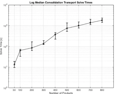
The problems were tested with a timeout of one hour. The MILP models were solved using Gurobi version 7.5.1 with Java version 1.8.0 on a 2.9 GHz Intel core i5 processor. Results can be seen in figure 2-2. The figure shows the median solve times for each problem size on a log scale with error bars covering the 25%-75% quartile ranges. Of the 20 problems generated for each of the problem sizes, all problems with sizes of up to 100 products were solved in under one hour, 18 with a size of 300 products were solved, 17 with a size of 400 products were solved, 19 with a size of 500 products were solved, 15 with a size of 600 products were solved, 12 with a size of 700 products were solved, and 17 with a size of 800 products were solved. The variability in the number of problems solved in under one hour for each problem size is due to the variability in problem parameteres generated, leading to more and less constrained problems. There are (𝑖𝑛𝑜𝑘 + 𝑖𝑛𝑜) binary decision variables in the consolidation transport model, so solve time increases less dramatically than in the manufacturing plant or distribution center problems. Although it is possible to solve problems involving many more products than the manufacturing plant model with the consolidation transport model, since it will be necessary to schedule production of on the order of thousands of products in the motivating supply chain example, the size of problem that can be solved here is still approximately one order of magnitude smaller than necessary for the real-world supply chain problem.
2.3.4
Limitations of the Consolidation Transport Model
While the consolidation transport model accounts for the vehicle packing and schedul-ing aspects of the consolidation transport process, there are a number of limitations in this model as compared with the real-world consolidation transport process. Much like the manufacturing plant model, the consolidation transport model is limited in its ability to manage uncertainty in execution, in this case caused by varying depar-ture times. This model also only considers one vehicle size, while in the real-world consolidation transport problem, there are two possible vehicle sizes available for each departure time on each day. In the real-world problem, the number of each type of vehicle to use is chosen based on daily shipping needs. Finally, during particularly
Figure 2-2: Log Median Consolidation Transport Model Runtimes
busy weeks, the consolidation transport process occasionally involves a step in which vehicles are packed and then parked at the distribution centers that they are depart-ing from in advance of their actual departure times. This step is not considered in this model.
2.4
Distribution Center
The distribution center problem is a capacity constraint problem with a temporal element. As products flow into and out of the distribution centers over time, facility capacity constraints must be met across the time horizon. There are two types of dis-tribution center including manufacturing plant disdis-tribution centers, where items that have completed production are collected to be grouped onto consolidation transport vehicles, and regional distribution centers, where items are collected from consolida-tion transport vehicles to be shipped to the final customer destinaconsolida-tion in a single shipment. The distribution center model assumes that if volumetric constraints are
met, items can be packed to fit in the distribution center and that there are no labor constraints associated with the number of items that can be handled in a distribution center. Currently, the model of the distribution center also assumes that there are no assigned arrival times or necessary departure deadlines, and these are instead deci-sion variables in the problem. In the integrated supply chain model, the distribution center arrival times and departure times for each product will correspond to other variables in the supply chain process. The consolidation transport vehicle arrival time will become a product’s arrival time at a regional distribution center and the outbound transport vehicle departure time will be its departure time from the center. The manufacturing plant production completion time will become a product’s arrival time at the manufacturing plant distribution center and the consolidation transport vehicle departure time will be its departure time from that facility. In the absence of these other variables, a minimum dwell time is imposed on products flowing through the distribution center.
2.4.1
Distribution Center Inputs, Outputs, Objective, and
Con-straints
The inputs to the distribution center problem include the list of products that will pass through the distribution center and their volumetric sizes and the volumetric capacity of the facility. The outputs of the problem are the product arrival and departure times at the distribution center. The objective is to minimize the sum of the wait times at the distribution center for all products. This objective is a stand-in objective for proof of concept, and in the integrated model, deadlines will be taken into consideration, and flow through the distribution center is simply a feasibility problem.
At a high level, the constraints in the distribution center model include the fol-lowing:
1. The distribution center facility capacity must not be exceeded when a product arrives at the facility.
2. Each product much spend a specified minimum amount of time at the distribu-tion center facility.
Constraint 1 ensures that facility capacity is never exceeded by making sure that capacity constraints are met each time a product arrives at the facility. Although both arrival times and departure times of each product are decision variables in the distribution center model, capacity could only ever be exceeded when a new product arrives at the facility and it was not there before, so this constraint applies only when products arrive. Constraint 2 is a stand-in constraint in the absence of the product manufacturing plant completion times and consolidation transport vehicle departure times that are present in the integrated problem. In the integrated model, product manufacturing plant completion times act as distribution center arrival times and consolidation transport departure times act as distribution center departure times for each product. Constraint 2 ensures that the arrival and departure times are not scheduled at the same time for each product in the absence of these incoming and outgoing constraints, which forces the products to remain at the distribution center for a nonzero amount of time and allows for the proof of concept for ensuring capacity constraints are met over time.
2.4.2
Distribution Center MILP Formulation
The formal distribution center problem MILP formulation is as follows:
𝑚𝑖𝑛∑︁ 𝑘∈𝐾 (𝑈𝑘− 𝑇𝑘) (2.38) 𝑍𝑘𝑚 ≤ 𝑀4· 𝑋𝑘𝑚 ∀ 𝑘, 𝑚 ∈ 𝐾 (2.39) 𝑍𝑘𝑚≤ 𝑇𝑚 ∀ 𝑘, 𝑚 ∈ 𝐾 (2.40) 𝑇𝑚+ 𝑀4· 𝑋𝑘𝑚− 𝑍𝑘𝑚 ≤ 𝑀4 ∀ ∈ 𝐾 (2.41) 𝑍𝑘𝑚 ≥ 0 ∀ 𝑘, 𝑚 ∈ 𝐾 (2.42) 𝑅𝑘𝑚− 𝑀4· 𝑋𝑘𝑚 ≤ 0 ∀ 𝑘, 𝑚 ∈ 𝐾 (2.43)
𝑅𝑘𝑚− 𝑈𝑚 ≤ 0 ∀ 𝑘, 𝑚 ∈ 𝐾 (2.44) 𝑈𝑚+ 𝑀4 · 𝑋𝑘𝑚− 𝑅𝑘𝑚 ≤ 𝑀4 ∀ 𝑘, 𝑚 ∈ 𝐾 (2.45) 𝑅𝑘𝑚 ≥ 0 ∀ 𝑘, 𝑚 ∈ 𝐾 (2.46) 𝑍𝑘𝑚− 𝑇𝑘 ≤ 0 ∀ 𝑘.𝑚 ∈ 𝐾 (2.47) 𝑀4· 𝑋𝑘𝑚+ 𝑇𝑘− 𝑅𝑘𝑚 ≤ 𝑀4 ∀ 𝑘, 𝑚 ∈ 𝐾 (2.48) 𝑀4· 𝐻𝑘𝑚− 𝑇𝑘+ 𝑇𝑚 ≤ 𝑀4𝑚𝑏𝑜𝑥 ∀ 𝑘, 𝑚 ∈ 𝐾 (2.49) 𝑀4 · 𝐻𝑘𝑚− 𝑇𝑘+ 𝑇𝑚 ≥ 𝜖 ∀ 𝑘, 𝑚 ∈ 𝐾 (2.50) 𝑀4· 𝐽𝑘𝑚− 𝑈𝑚+ 𝑇𝑘 ≤ 𝑀4 ∀ 𝑘, 𝑚 ∈ 𝐾 (2.51) 𝑀4· 𝐽𝑘𝑚− 𝑈𝑚+ 𝑇𝑘 ≥ 𝜖 ∀ 𝑘, 𝑚 ∈ 𝐾 (2.52) 𝐻𝑘𝑚+ 𝐽𝑘𝑚− 𝑋𝑘𝑚 ≤ 1 ∀ 𝑘, 𝑚 ∈ 𝐾 (2.53) 𝑋𝑘𝑚 ≤ 1.0 ∀ 𝑘, 𝑚 ∈ 𝐾 (2.54) ∑︁ 𝑚∈𝐾 𝑝𝑟𝑜𝑑𝑢𝑐𝑡𝑆𝑖𝑧𝑒𝑠𝑚· 𝑋𝑘𝑚 ≤ 𝑓 𝑎𝑐𝑖𝑙𝑖𝑡𝑦𝑆𝑖𝑧𝑒 ∀ 𝑘 ∈ 𝐾 (2.55) 𝑈𝑚− 𝑇𝑚 ≥ 𝑚𝑖𝑛𝑇 𝑖𝑚𝑒 ∀ 𝑚 ∈ 𝐾 (2.56)
Here, 𝑘, 𝑚 ∈ 𝐾 are products in the total set of products 𝐾. 𝑇𝑘 ∈ [0, ℎ𝑜𝑢𝑟𝑠𝑃 𝑒𝑟𝑆ℎ𝑖𝑓 𝑡]
is a decision variable that represents the the arrival time of product k at the distribu-tion center. 𝑈𝑘∈ [0, ℎ𝑜𝑢𝑟𝑠𝑃 𝑒𝑟𝑆ℎ𝑖𝑓 𝑡] is a decision variable representing the departure
time of product k at the distribution center. 𝑋𝑘𝑚 ∈ {0, 1} is a linearizing binary
de-cision variable that takes the value of one if product m is at the distribution center when product k arrives and zero otherwise. 𝑅𝑘𝑚∈ Z, 𝑍𝑘𝑚∈ Z, 𝐻𝑘𝑚 ∈ {0, 1}, and
𝐽𝑘𝑚 ∈ {0, 1} are linearizing decision variables used to linearize constraints.
Equation 2.38 is the objective and minimizes the total product dwell time at the distribution center across all products. Equations 2.39-2.41 are linearizing equations to set 𝑍𝑘𝑚 = 𝑋𝑘𝑚· 𝑇𝑚. Equations 2.42-2.46 are linearizing equations to set 𝑅𝑘𝑚 =
center before product 𝑚. Equation 2.48 ensures that 𝑋𝑘𝑚 = 0 if product 𝑚 leaves the
distribution center before product 𝑘 arrives. Equations 2.49-2.54 ensure that 𝑋𝑘𝑚 = 1
if product 𝑚 is at the distribution center when product 𝑘 arrives and product 𝑚 leaves the distribution center after product 𝑘 arrives. Equation 2.55 enforces constraint 1, and equation 2.56 enforces constraint 2.
2.4.3
Distribution Center Results and Discussion
Like the consolidation transport model, the distribution center model was evaluated using a state-of-the-art optimizer, Gurobi, to serve as a step towards developing an integrated model and evaluating where primary bottlenecks are in an integrated model. The distribution center model was evaluated with a constant volumetric size of 50 cubes (the unit used in the motivating supply chain example) while varying the number of products from one through the maximum for which a majority of problems could be solved in a time limit of one hour, which was 11. The volumetric size for the distribution center is set such that the ratio of facility size to product size and the number of products that fit in the facility at any given time is lower than is true to the motivating supply chain example. This was such that some small problems, like the ones included in the results for this section, could be run and completed before a one hour timeout and the trends of the results could be obtained. Problem sizes of two, five, eight, nine, 10, and 11 products were tested. For each of these cases, 20 sets of problem parameters were randomly generated including product sizes sampled from a uniform distribution between zero and five (with units of cubes).
The problems were tested with a timeout of one hour. The MILP models were solved using Gurobi version 7.5.1 with Java version 1.8.0 on a 2.9 GHz Intel core i5 processor. Results can be seen in figure 2-3. The figure shows the median solve times for each problem size on a log scale with error bars covering the 25%-75% quartile ranges. Of the 20 problems generated for each problem size, all problems with sizes of up to nine products were solved in under one hour, 18 problems with a size of 10 products were solved, and 16 problems with a size of 11 products were solved. This problem has 3𝑘2 binary decision variables and (2𝑘 + 2𝑘2) continuous decision
Figure 2-3: Log Median Distibution Center Model Runtimes
variables. The quadratic increase in number of decision variables likely corresponds to the dramatic increase in solve time as number of products is increased. Here, the maximum problem size that is solvable within an hour timeframe is 11 products, two orders of magnitude smaller than the real-world problem sizes in the motivating supply chain example. Since this problem size is smaller than the problems solved by both the manufacturing plant and consolidation transport models, the distribution center aspect of the integrated model is likely the bottleneck in the size of problem that can be solved with that model.
2.4.4
Limitations of the Distribution Center Model
The distribution center model accounts for capacity constraints over time as products move into and out of distribution center facilities. As with the previously discussed models, the distribution center model is limited in its ability to account for uncertainty in execution times as products arrive and depart facilities. It is also limited in the fact that it does not account for the labor requirements associated with moving products
into and out of distribution centers, involving the unloading and reloading of products onto transport vehicles. In the real-world, labor requirements could prove to be a bottleneck in addition to facility capacity.
2.5
Integrated Model
The integrated model integrates one manufacturing plant, one plant distribution cen-ter, and one set of consolidation transport vehicles scheduled from the plant distri-bution center to one regional distridistri-bution center. There are constraints that connect each of the models together, setting the completion time at the manufacturing plant to distribution center arrival time and the consolidation transport vehicle departure time to the distribution center departure time for each product. In the integrated model, there is no longer a constraint on minimum stay time at the distribution center for each product since arrival and departure times are determined by the other steps in the process previously mentioned. Therefore, equation 2.56 is not present in the integrated model.
Similar to the manufacturing plant model, the objective in the integrated model is to minimize the lateness, or the time before or past the deadline that the product is completed, and total labor required across the time horizon. In this case, the dead-line for each product corresponds to a deaddead-line for departing the distribution center on a consolidation transport vehicle, as opposed to it being a manufacturing plant completion time as was the case in the manufacturing plant model. The objective can be expressed as:
𝑚𝑖𝑛 ∑︁ 𝑖∈𝐼,𝑗∈𝐽,𝑙∈𝐿 𝑌𝑖𝑗𝑙+ ∑︁ 𝑘∈𝐾 𝐸𝑘 (2.57)
The linking constraints that are added include:
∑︁ 𝑖∈𝐼,𝑛∈𝑁,𝑜∈𝑂 (ℎ𝑜𝑢𝑟𝑠𝑃 𝑒𝑟𝑆ℎ𝑖𝑓 𝑡 ·⌊︁𝑛 3 ⌋︁ + 𝑑𝑒𝑝𝑎𝑟𝑡𝑢𝑟𝑒𝑇 𝑖𝑚𝑒𝑠𝑛 mod 3) · 𝐵𝑖𝑛𝑜𝑘− 𝐶𝑘 = 0 ∀ 𝑘 ∈ 𝐾 (2.58)