HAL Id: hal-01076659
https://hal.archives-ouvertes.fr/hal-01076659
Submitted on 22 Oct 2014
HAL is a multi-disciplinary open access
archive for the deposit and dissemination of sci-entific research documents, whether they are pub-lished or not. The documents may come from teaching and research institutions in France or abroad, or from public or private research centers.
L’archive ouverte pluridisciplinaire HAL, est destinée au dépôt et à la diffusion de documents scientifiques de niveau recherche, publiés ou non, émanant des établissements d’enseignement et de recherche français ou étrangers, des laboratoires publics ou privés.
Iso-scallop tool path generation in 5-axis milling
Christophe Tournier, Emmanuel Duc
To cite this version:
Christophe Tournier, Emmanuel Duc. Iso-scallop tool path generation in 5-axis milling. Interna-tional Journal of Advanced Manufacturing Technology, Springer Verlag, 2005, 25, pp.867 - 875. �10.1007/s00170-003-2054-7�. �hal-01076659�
Iso-scallop tool path generation in 5-axis
milling
CHRISTOPHE TOURNIER*, EMMANUEL DUC**
* LURPA - Ecole Normale Supérieure de Cachan, 61 avenue du Président Wilson, 94235 Cachan Cedex, France ([email protected])
** LARAMA - Institut Français de Mécanique Avancée, Campus de Clermont Ferrand, 63175 Aubière Cedex, France ([email protected])
Abstract:
This paper presents a new method of computing constant scallop height tool paths in 5-axis milling on sculptured surfaces. Usually, iso-scallop tool paths computation methods are based on approximations. The attempted scallop height is modelled in a given plane to ensure a fast computation of the tool path. We propose a different approach, based on the concept of the
machining surface, which ensures a more accurate computation. The machining surface defines
the tool path as a surface, which applies in 3 or 5-axis milling with the cutting tools usually used. The machining surface defines a bi parametric modelling of the locus of a particular point of the tool, and the iso-scallop surface allows to easily find iso-scallop tool centre locations. An implementation of the algorithms is done on a free-form surface with a filleted endmill in 5-axis milling.
Keywords:
5-axis milling, free-form surfaces, filleted endmill, machining surface, constant scallop height.
Symbols:
SSh constant scallop height surface
Sn CAD surface
MS machining surface
sh scallop height (mm)
Cc cutter contact point
CL cutter location point
P point onto the scallop curve
K cutter location point on the guiding surface
n surface normal f tool feed vector t tangent to the surface u tool axis vector
R tool radius (mm)
r tool corner radius (mm)
θt tilt angle
θn yaw angle
ξ1
Introduction
The manufacturing process of sculptured surfaces is an important issue in aeronautic, mould and die industries. This process is based on 3 or 5-axis end milling and consists in the sweeping of the surface by the tool. The process must produce parts respecting the functional requirements and reduce machining time. In particular, the machining strategy has a great influence on the machining time and the effective roughness.
The sculptured surface realization process is based on the followings steps: - the numerical definition of the part in a CAD software ;
- the computation of the necessary tool paths in a CAM software ; - the effective realization of the part by means of a machine tool ;
- the measurement of the part and the checking of the respect of the awaited quality level.
The machining tool path defines all the positions which have to be reached by the tool in a given description format, so that the surface generated by sweeping respects the geometrical specifications of form deviation and roughness. This trajectory is thus a geometrical model associated to the CAM activity: the CAM model. Its geometrical richness makes it more or less relevant.
We can define another geometrical model used in the process: the virtual manufactured model. The transformation from the CAM model to the virtual manufactured model is obtained by the computation of the envelope surface. The envelope surface of the tool movement is the skin of the volume swept by the tool during its displacement along the path. More generally, according to [1],[2],[3] one regards as swept volume the volume generated by a solid object displacement along an unspecified trajectory with possible rotations. The equation of the envelope surface can be simple, for example in the case of the skin of the volume swept by a sphere. The envelope surface of the tool movement is a pipe surface of radius equal to the tool radius and whose generator is the curve followed by the cutter location point CL. The extraction of the equation of the swept volume surface is a difficult operation especially when it presents self-intersections. Extracting the equation of the envelope surface of a filleted tool is thus not considered. On the other hand, at every moment the locus of the generating profile
points of the envelope surface, and for any tool [2] is defined by the next equation: 0 tool = ⋅ n V (1)
with V the speed vector and ntool the tool normal vector at the considered point. This equation will help us to determine the points generated by the tool on the part and especially the scallop points.
To compute a tool path respecting the above mentioned specifications, we have to plan the tool path by choosing a tool driving direction and the transversal and longitudinal discretization steps [4]. Along the machining direction, i.e., the longitudinal direction, the calculated tool path must lead to the respect of the dimensional and form deviations specifications. From the exact theoretical tool path that perfectly machines the surface, we can build a pipe whose diameter is lower than the specification of form deviation. The calculated tool path must be contained in this pipe. The computed tool path is the modelization of the theoretical tool path according to a chosen interpolation format. This is significant regarding the machined surface quality and the effectiveness of the machine tool. If one controls the tool by linear interpolation, the distance between the tool locations must be sufficiently weak to respect the tolerance of form deviation [4]. But that can produce facets on parts with large curvature radii. Then, we must add interpolation points where the tool path presents large curvature radii. However a too small distance between following points limits high speed machining performances because of the processing time of the NC code by the numerical control units [5]. The use of polynomial interpolators in the development of tool path generators brings a better solution to this problem. Tool paths described in the polynomial format do not generate facets and the machine tool reaches the expected feedrate easier. On the other hand, it is essential to detect discontinuities during the calculation of the tool paths [6].
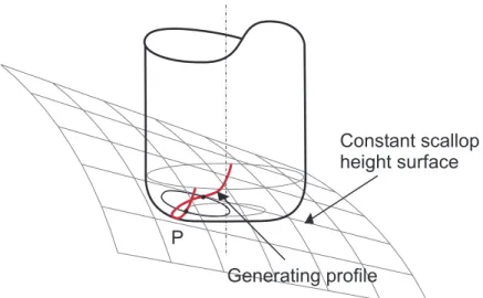
In the transversal direction, the distance between two consecutive tool paths must be sufficiently weak so that the specifications of form deviation and roughness are respected all over the part. According to the tools geometry, the specified roughness defines a maximum scallop height sh. We can thus define the constant scallop height surface SSh, which is the offset surface of the design surface with a magnitude equal to the maximum scallop height. In order to machine the expected surface with the right specifications, all the scallops generated by the successive
tool paths must lie between the CAD surface and the constant scallop height surface SSh.
In fact, it should be noticed that the problem is not so uncoupled. It has been showed that the precision of the tool path in the longitudinal direction has an influence on the transversal profile. Indeed, the tool contact points, along two adjacent tool paths, are not always synchronized in the transversal direction. In this case the transversal profile of the machined surface is not composed of the same scallops, lying perfectly on the CAD surface, but of a succession of more or less deep scallops [7].
The machining strategy plays a significant role on the respect of roughness.With the conventional strategies where the tool is driven along parallel planes or iso-parametric curves on the surface, only the maximum scallop height can be managed between two adjacent tool paths. To be able to control the scallop height on a specific area, we have to tighten the entire tool path. Then, scallops left on the part are lower than the expected limit almost all over the part. In order to improve the machined surface quality and to potentially minimize machining time, we can use the constant scallop height tool path strategy.
This strategy, also called the iso-scallop strategy [8], ensures that scallops on the part will be evenly distributed. It has been showed that this machining strategy optimizes the sweeping of the surface by the tool [9]. In a constant scallop height strategy, the scallop curve is lying on the constant scallop height surface SSh. Starting from an initial tool path, we find the intersection curve of the swept volume with the constant scallop height surface. Then, based on the found scallop curve, we compute the next tool path [14],[15]. In 3-axis milling, several approaches have been developed to compute iso-scallop tool paths with ball endmill [9],[10],[11]. Tool paths are planned in the parametric space of the CAD surface and the two first fundamental forms are used to evaluate the surface properties at the considered point. In 5-axis milling, two methods have been developed, one for the filleted endmill [12] and another one for the flat endmill [13]. This last method is quite similar to those developed for the 3-axis milling because the effective cutting profile of the tool is approached by a circle in the plane normal to the tool path. We compared our approach, [14], with those founded in the literature and showed that our method were more precise in terms of scallop height as well as more efficient on curvature discontinuities.
Now, our objective is to apply our method [14] in the case of 5-axis milling with a filleted endmill. The proposed method is based on the use of the concept of the machining surface. We consider that the surface is the most accurate model to compute high quality tool paths, to respect the expected quality and to take into account the connection between the longitudinal and transversal steps. It would bring an enrichment to facilitate the generation of iso-scallop tool paths because the gap between two adjacent tool locations is filled by a surface element [16],[17]. The Machining Surface (MS) is a surface including all the information necessary for the driving of the tool, so that the envelope surface of the tool movement sweeping the MS gives the expected free form.
We will initially present in detail the concept of the machining surface and the geometry of the machining surface in 3 and 5-axis milling. Then, we will focus on the calculation of the iso-scallop tool paths. An application of the approach is proposed at the end of the paper.
The concept of the machining surface
The machining surface can be characterized as a biparametric space gathering all the information required to build a tool path. The shape of the machining surface must lead to the respect of the design intent, whatever the adopted machining strategy.
The sampling phase from the CAD surface to the set of discrete CL points generates geometric deviations between the envelope of the tool movement and the CAD surface. The two-dimensional and continuous approach suggested by the machining surface prevents the degenerating of the CAD model in a set of points. Our objective is to build a surface on which we can compute curves as tool paths, according to the design intents and a machining strategy. The definition of the machining surface depends on whether the machining is performed in 3 or 5-axis milling and on the tool geometry.
Machining surface in 3-axis milling: the MS is the surface P(u,v), locus of a particular point of the tool (centre or extremity), so that the free-form
corresponds to the envelope surface of the tool movement when the particular point is sweeping the MS
In 3-axis milling, the machining surface is the generalized offset surface. These offset surfaces have been already used to compute tool path especially with ball
endmills [18], [19] but also with flat and filleted endmills [20]. We focused on the definition of the MS in 5-axis end milling.
Machining surface in 5-axis milling: the MS consists in a couple of surfaces P(u,v) and Q(t,w), with P(u,v) following the previous definition, so that for each point P of P(u,v), there exists a point Q on Q(t,w), so that PQ defines the direction of the tool axis.
We now develop the geometrical model of the machining surface. In order to deal with a general case, let us consider the 5-axis milling with a filleted endmill. Then we will extrapolate the results to the other tool geometries.
Fig. 1: Here
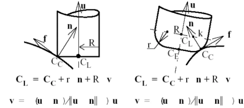
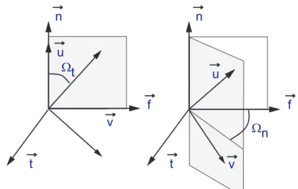
In 3-axis milling, we are able to drive the tool centre location point CL and to find the resulting tool contact point CC like in the offset [18] and APT approaches. But this approach has not been applied in 5-axis milling due to its complexity [21]. Hence, the tool path generation in 5-axis milling usually consists in computing the tool center location CL and the tool axis vector u for each tool contact point CC between the tool and the surface along the tool path [22], [23]. To ensure the tangency between the tool and the machined surface and avoid gouging, the tool can be rotated around the two vectors t and n of the local coordinate frame defined by: (CC, f, n ,t) where: f is the tool feed vector, n the vector normal to the surface and t the vector tangent to the surface with t = f ∧ n. We propose to change theses rotations (θt, t) and (θn, n) and to define these in the local coordinate frame (K, f, n, t), with K located on the meridian circle of the torus defined by:
n C
C
K= + r⋅ (2)
K belongs to the instantaneous rotation vector of the tool. It thus remains fixed during the rotational movements of the tool. The rotations ensure a tangent contact between the tool and the part. It also should be made sure that the two rotations leave the tangent planes of the tool and surface confused at the contact point CC. Regarding to the rotation (θn, n), the result is immediately proved because n is orthogonal to the tangent plane. For the second rotation, obtaining the result has to be proved. We first of all define the position of the tool by defect as being that for θt = θn = 0 when :
- vectors u and n are parallels, - u is in the plane defined by (K, f, n)
This configuration ensures a tangent contact because in any contact point CC between the tool and the surface, the normal on the surface passes by the axis of the torus. The demonstration is described in appendix A.
Fig. 2: Here
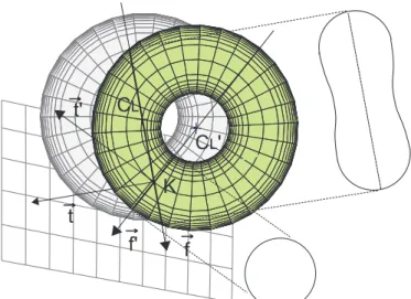
Consider C, the circle resulting from the intersection between the torus
representing the active part of the tool and the plane (K, f, n). This plane passing
by the axis of the torus, C is the circle of centre K which generates the torus by
rotation around the meridian circle. The vector t is orthogonal to the circle C because orthogonal to (K , f , n) by definition. The rotation around t thus leaves
the circle C identical to itself. Therefore, the active part of the tool remains
tangent on the surface, only the contact point, belonging to the tool is modified. The contact point CC belonging to the surface is unchanged, the tool always machines the same point.
However, the order of rotations is significant to preserve a tangent contact. If the rotation (θt, t) takes place in first, the point CC remaining unchanged, the normal n is also unchanged. The second rotation (θn, n) thus leaves the tangent planes confused. On the other hand if (θn, n) is the first rotation, the plane (K, f, n) is not any more the meridian plan of the torus and the intersection between the torus and this plane is an oval of Cassini (Fig. 2). Consequently the rotation around t does not leave any more the active part of the tool identical to itself, an interference occurs. In this case, the rotation must be done around the vector t’, image of the vector t by rotation (θn, n).
Fig. 3: Here
We decide to retain the point K to calculate the tool location but we should define
at least a second fixed point of the tool. For that we will use the point CL such as v = KCL (Fig. 1). With two points to locate the tool, there remains a possible rotation around the vector v . However, it should be noticed that the tool axis vector u, the vector v and the normal vector n passing through CC remain always coplanar during the two rotations (θt, t) and (θn, n). Indeed, they are coplanar since the beginning of the setting in position because at any point CC, the normal
to the surface passes by the axis of the torus. Then, the two rotations (θt, t) and (θn, n) leave the vectors u, v, n coplanar (Fig. 3). Knowing points K, CL and the
normal vector n is sufficient to position the tool in the 3D space. The tool axis vector is then defined by:
v n v n v u ∧ ∧ ∧ = (3)
The points K and CL define a unique tool position because they are located in the symmetry plane of the tool.
Fig. 4: Here
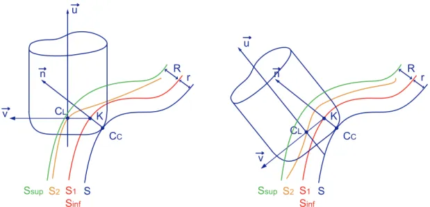
The MS is thus composed of two surfaces S1 and S2, loci of the points K and CL (Fig. 4). We call the surface S1 the guiding surface and surface S2 the orientation surface. The guiding surface S1 is the offset surface of the nominal surface with magnitude equal to the corner radius r of the tool. It is thus independent of the
machining strategy. The orientation surface S2 is the surface that gives the orientation of the tool axis according to the considered machining strategy.
From the CAD surface Sn described by the parametric function F(ξ1,ξ2), we can determine the parametric function of the guiding surface S1, Fgui(ξ1,ξ2) :
( ) ( )
1 2 1 2( )
1 2 , . , ( , (ξ ξ ξ ξ r nξ ξ gui = F + F (4)The orientation surface is built according to the orientation we wish to give to the tool along the tool path. The orientation of the tool axis is described by u(ξ1,ξ2).
One can evaluate the parametric function Fori(ξ1,ξ2) of the orientation surface S2 followed by the centre of various types of tools. The results obtained in the case of 5-axis milling with a filleted endmill can be extended to the other tool geometries. The flat endmill can be described as a filleted endmill with a corner radius r null.
Thus, K coincides with the cutter contact point CC and the surface S1, locus of the points K is the nominal surface to be machined. In this case, the machining
strategy controls the cutter contact point. The ball endmill can be considered as a filleted endmill with a principal radius R equal to zero. The point K then coincides
with the point CL. The adopted solution that uses points K and CL is not valid for this type of tool. Thus, we use the standard configuration with the parameters CL and u.
The following table presents all the definitions of the guiding and orientation surfaces, according to the used machine and tool.
3-axis 5-axis Filleted endmill S1 : F + r n S1 : F + r n S2 : F + r n + u Ball endmill S1 : F + R.v S1 : F S2 : F + R.v Flat endmill S1 : F + r.n + R.v S1 : F + r n S2 : F + r n + R.v
Iso-scallop tool path generation in 5-axis machining
We first recall that 5-axis machining with a filleted endmill allows to get different machining strip width regarding the tool axis orientation. Indeed, the effective cutting profile is an ellipse. The minor and the major axes and radii depend on the tilt and yaw angles. The local radius of the effective cutting profile Reff is equal to [23]: 2 2 ( sin ) sin cos sin ) sin ( n t n t t eff θ θ θ θ R rθ r r R r R + ++ = (5)
To be as effective as possible, the iso-scallop tool path strategy must be linked to minimum tool axis orientation angles. In 5-axis milling, the MS is made of two
surfaces, the guiding and the orientation surface. The guiding surface can be directly computed from the initial surface. But the orientation surface cannot be defined before the end of the tool path generation. Its construction depends on the tool axis orientation, which is defined with the tool feed direction. But the tool feed direction will be found during the tool path generation. So we only use the guiding surface to compute iso-scallop tool path, the corner radius offset surface. The orientation surface may be used to modify the tool axis orientation to avoid gouging after the iso-scallop computation.
Computing a scallop point
The computation of the tool positions proceeds in two stages. During the first stage, we try to find the scallop point P associated with an initial position of the
cutter location point K. The geometrical conditions to respect are as follows :
- P is belonging to the constant scallop height surface SSh:
)
,
(
)
,
(
ξ
1ξ
2n
ξ
1ξ
2P
=
S
n+
s
h⋅
(6)surface equation (the next equation is given for a tool axis oriented along the Z
axis):
(
) (
) (
)
(
P−CL 2x+ P−CL2y+ P−CL2z+R2−r2)
2−4R2(
(
P−CL) (
2x+ P−CL)
2y)
2=0 (7)- P is on the generative profil of the tool which creates the scallop curve:
(
V ⋅ntool)
P =0 (8)V is the speed of the considered point P belonging to the tool. Fig. 5: Here
We thus have a non-linear system of three equations with three unknown factors
Px, Py, Pz that yields a non-linear system of two equations in the two unknowns (ξ1, ξ2) in the parametric space of the CAD surface.
The resolution of the system can be done with the Newton algorithm, the difficulty is the determination of an initial solution which ensures convergence. We consider as an initial solution the preceding scallop point and to walk on the intersection between the constant scallop height surface SSh (6) and the toric tool (7) until the equation (8) is checked (Fig. 5).
Consider the intersection between the constant scallop height surface SSh and the toric tool. One of the surfaces, SSh, is a bi-parametric surface Fsh(ξ1,ξ2) and the other is described as an implicit surface St(X, Y, Z) = 0.
The mathematical formulation of this intersection problem is to find zeros of the function G (from [0,1]2 to ú3) : G(ξ1,ξ2) = St(Fsh(ξ1,ξ2)X, Fsh(ξ1,ξ2)Y, Fsh(ξ1,ξ2)Z) The non linear equation G(ξ1,ξ2) = 0 presents 2 unknowns (ξ1,ξ2). The solution is
a 3D parametric curve C with C(τ) = FSh(ξ1(τ),ξ2(τ)). The objective is not to compute the curve C but to keep marching on this curve.
Fig. 6: Here
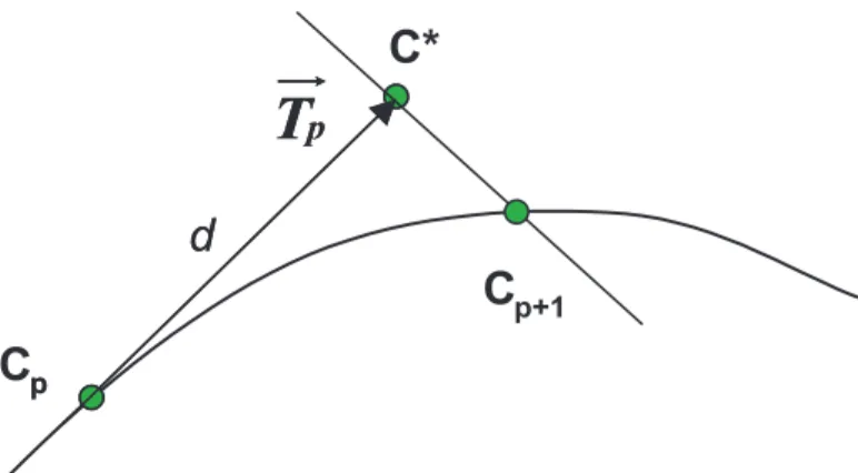
Marching on the curve is done with the marching method algorithm, including 3 steps: prediction, correction and progression (Fig. 6).
Prediction consists in doing a step of a distance d in the direction of the tangent Tp to the curve C(τ) at the point Cp. This way we find a valuable approximation C* of the solution Cp+1. We can write:
> − < = + = +1 p p p p p p , C C sign s . d . S C * C T T T (9)
During the correction step, the following point Cp+1 is computed based on the prediction point C*. Cp+1 is built as the intersection between C(τ) and the hyper-plane normal to the prediction direction, Tp passing thru C*.
d C Cp− p 1 >= < = + P P T T C , 0 ) (τ (10)
The progression distance d must be evaluated regarding the normal curvature of
C(τ) to optimize computing time. For each step along the curve C(τ), we check if
equation (8) is solved. It is then necessary to compute the speed vector of the considered point Cp belonging to the tool. The speed of a point M of the tool is computed by the next formula:
0 R tool / Ω MK V VM= K+ ∧ (11)
with K the point of the tool belonging to the guiding surface and Ωtool /R0 the
instantaneous speed rotation vector of the tool in its motion along the surface. In 3-axis milling, this vector is null because the tool axis stay parallel to the Z axis of the machine tool. But in 5-axis milling, the tool is oriented in the local coordinate system R1 defined by (K, f, n, t), and furthermore, this local coordinate system evolves all along the tool path.
We can write: 0 1 1 0 tool R R R R tool/ Ω / Ω / Ω = + (12) 1 / R tool
Ω is defined by the tool orientation angles chosen by the user and:
n t
Ωtool/R1 =θt. +θn. (13)
To compute the instantaneous speed rotation vector ΩR /1 R0, we use the next
formula which proof is given in appendix B:
) ( . 2 1 0 / dt d dt d dt d R R1 n n t t f f Ω = ∧ + ∧ + ∧ (14)
In kinematics, the variable t represents time but in our application, t is the parameter of the tool path curve followed by K.
The two vectors aα defined as follows belongs to the tangent plane to the guiding surface: 2 , 1 = = α ξα α d dFgui a (15)
They define the natural covariant base of the tangent plane. The surface normal vector n is computed as the vector product of the two derivatives aα. We use this base to compute ΩR /1 R0.
Once the scallop point is determined, the tangent to the scallop curve in each scallop point P is given by the vector product of the normals of the tool and the scallop height surface.
Computing the cutter location point of the next path
At the time of the second stage, the problem is to find the position of the cutter location point K on the guiding surface. The tool located on K has to generate the previous scallop point P while remaining tangent to the scallop curve and the CAD surface. Since the tool is generating the scallop point P, P must be located on the generative profile of the tool. Furthermore, the previous scallop curve is the intersection between the tool motion and the scallop surface. The tool normal vector is then perpendicular to the scallop curve tangent vector in P.
The new system of equation to solve is the following: - K belongs to the guiding surface SG
)
,
(
)
,
(
ξ
1ξ
2n
ξ
1ξ
2K
=
S
n+
r
⋅
(16)- the scallop point P belongs to the tool
(
) (
) (
)
(
P−CL 2x+ P−CL2y+ P−CL2z+R2−r2)
2−4R2(
(
P−CL) (
2x+ P−CL)
2y)
2=0 (17)- P is on the generative profil of the tool
(
V ⋅ntool)
P =0 (18)- The tool normal vector is perpendicular to the scallop curve tangent vector
(
T ⋅ntool)
P =0 (19)If the system is solved in the parametric space of the CAD surface, it becomes a [3 x 3] system which unknowns are the parametric coordinates (ξ1
,ξ2) of the driven point K, and the tool feed direction f. This direction is parameterised by an angle θ in the guiding surface tangent plane defined by vectors aα.
In 3-axis milling, the tool feed direction results from two tangency conditions between the CAD surface and the scallop itself. In 5-axis milling, the tool feed direction must lead to the respect of these conditions, while taking into account the curvature evolution of the CAD surface, that is to say, the instantaneous speed rotation vector ΩR /1 R0.
The system is solved using the Newton algorithm. The initial solution is computed as the symmetric of the tool location point on the previous tool path. The symmetry plane pass through the scallop point P and contains the tangent to the scallop curve and the normal vector to the CAD surface.
Fig. 7: Here
Implementation and example.
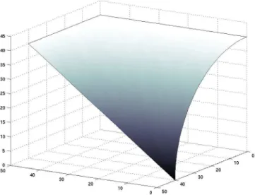
The implementation of the algorithm has been done on a personal computer under Linux operating system with the Matlab programming language. The test surface is a ruled Nurbs surface based on an arc of circle and a segment of straight lines (Fig. 7). We used an object approach to compute the characteristics of the Nurbs surface based on the algorithms developed in [24]. The tool radii are R = 10 mm and r = 1.5 mm and the scallop height is set to 10 µm. The first tool path is the right isoparametric boundary of the surface.
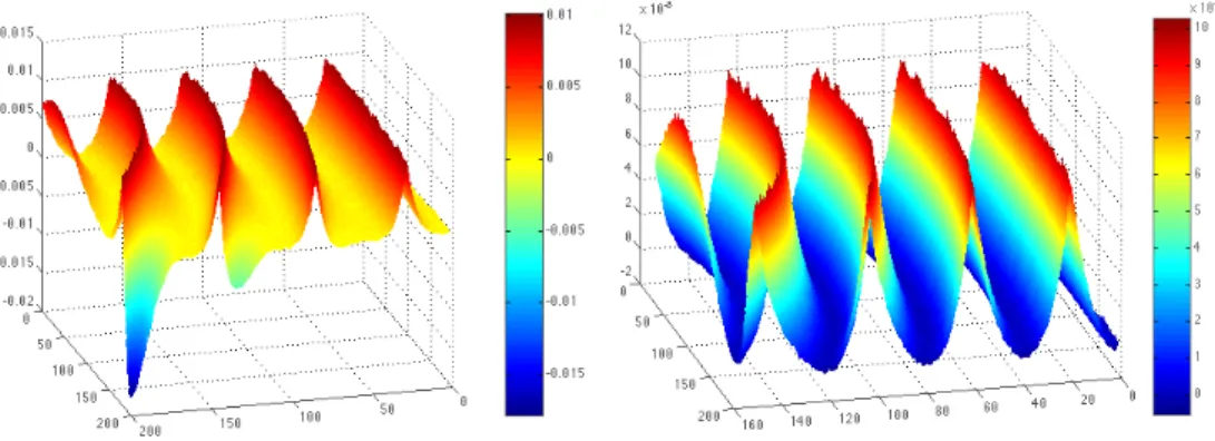
To evaluate the scallop height, scallops left by the tool are built with the method of the Z-buffer. We build in the studied zone a network of parallel straight lines and laid out on a grid which step indicates the precision. Then, we carry out the intersections between this network of lines and the envelope surfaces of the movement of the tool, the tool moving along line segments interpolating the calculated path. Lastly, one calculates the distance between each point of intersection and the machined surface.
Fig. 8: Here
We first applied our approach with a tilt angle of 1 degree. The scallops were consistent with the specifications but interferences appeared between the tool an the part in the concave area (Fig. 8). We can remove these interferences by using a tilt angle of 2 degrees all over the part. The specification of scallop height is always respected, interferences are removed but the tool paths are tightened since the machining strip width is smaller with a tilt angle of 2 degrees.
Conclusion and future works
We have developed the concept of the Machining Surface to get a continuous representation of the tool path and also to improve the machined surface quality by associating directly the MS to the design constraints (this part of the concept is not presented in the paper). The bi-parametric representation of the tool path used by the offset tool path generation methods for 3-axis is extended to 5-axis milling. The MS is made of the guiding and the orientation surfaces which allows to uncouple the respect of design and dynamics constraints. Based on the bi-parametric representation of the tool path, we developed a method of computing constant scallop height tool path in 5-axis milling with a filleted endmill. The concept of the machining surface appears as an excellent support to compute constant scallop height tool path because it enables us to use various geometries of tool while preserving the same mathematical formulation. We succeed to apply our method in 3-axis milling for the filleted and ball endmill. However, it does not apply for the cylindrical tool because of the discontinuity in tangency caused by the edge of the tool.
The method is thus reliable to compute constant scallop height tool path. Nevertheless, effective calculation is conditioned by the CAD surface. We showed that the form of the tool path generated by the constant scallop height strategy is prone to the variations of curvature of the machined surfaces, which can prevent the result of calculation. The aim of our current work is about analysing more in detail the difficulties of constant scallop height tool path planning. Since our computation is based on sampled points on the first path, the convergence of the calculation depends on the choice of the first path. Furthermore, the density of points on each path depends on the sampled on the first one.
References
[1] Abdel-Malek K., Yang J., Blackmore D, (in press) “On Swept Volume Formulations: Implicit Surfaces, Computer Aided Design”.
[2] Chiou C.J., Lee Y.S., “A shape-generating approach for multi-axis machining G-buffer models”, Computer-Aided Design, vol. 31, p. 761-776, 1999.
[3] Roth D., Bedi S., Ismael F., Mann S., “Surface swept by a toroidal cutter during 5-axis machining”, Computer-Aided Design, vol. 33, p. 57-63, 2001.
[4] Choi, B. , Jerard, R., “Sculptured Surface Machining - Theory and Applications”, Kluwer Academic Publishers, 1998.
[5] Valette, L., Duc, E., Lartigue, C, “A method for computation and assessment of NC tool paths in free-form curve format”, Int. Seminar on Improving Machine Tool performance, La baule (France), 3-5 Juillet 2000.
[6] Duc E., Lartigue C., Laporte S., “Assessment of the description format of tool trajectories in 3-axis HSM of sculptured surfaces”, Metal Cutting and High Speed Machining, edited by D. Dudzinski, A. Molinari, and H. Schluz – Kluwer Academic / Plenum Publishers, 2002.
[7] Lartigue C., Duc E., Tournier C., “Machining of free-form surfaces and geometrical specifications”, IMechE Journal of Engineering Manufacture, vol. 213, pp.21-27, 1999.
[8] Chiou C.J, Lee Y.S, “A machining potential field approach to tool path generation for multi-axis sculptured surface machining”, Computer-Aided Design, vol. 34, p. 357-371, 2002.
[9] Suresh K., Yang D.C.H., “Constant scallop-height machining of free-form surfaces”, Journal of Engineering for Industry, vol. 116, May 1994.
[10] Sarma R., Dutta D., “The Geometry and Generation of NC Tool Paths”, Journal of Mechanical Design, vol. 119, 1997.
[11] Lin R-S., Koren Y., “Efficient tool-path planning for machining free-form surfaces”, Journal of Engineering for Industry, vol. 118, February 1996.
[12] Lee Y.S., “Non isoparametric tool path planning by machining strip evaluation for 5-axis sculptured surface machining”, Computer-Aided Design, vol. 30, no. 7, p. 559-570, 1998.
[13] Lo C-C., “Efficient Cutter-path planning for five-axis surface machining with flat-end cutter”, Computer-Aided Design, vol. 31, no. 9, p.557-566, 1999.
[14] Tournier C., Duc E., “A surface based approach for constant scallop height tool path generation”, The International Journal of Advanced Manufacturing Technology, vol 19, pp. 318-324, 2001
[15] Feng H-Y., Li H., “Constant scallop-height tool path generation for three-axis sculptured surface machining”, Computer-Aided Design, vol 34, no 9, pp 647-654, 2002.
[16] Duc E., Lartigue C., Tournier C., Bourdet P., “A new concept for the design and the manufacturing of free-form surfaces: the machining surface”, Annals of the CIRP, vol. 48/1, pp. 103-106, 1999.
[17] Tournier C., Duc E., Lartigue C., Contri A. ,”The concept of the machining surface in 5-axis milling of free-form surfaces”, Selected papers of the conference IDMME’2000, Kluwer academic publisher, 2002.
[18] Kim K.I., Kim K., “A new machine strategy for sculptured surfaces using offset surface”, International Journal of Production Research, vol. 33, no. 6, p. 1683-1697, 1995.
[19] Lartigue C., Thiebaut F., Maekawa T., “CNC tool path in terms of B-spline curves”, Computer-Aided Design, vol. 33, no. 4, p. 307-319, 2001.
[20] Hwang J.S., Chang T.C., “Three-axis machining of compound surfaces using flat and filleted endmills”, Computer-Aided Design, vol. 30, no. 8, p. 641-647, 1998.
[21] Li S.X., Jerard R.B., ”5-axis machining of sculptured surfaces with a flat-end cutter”, Computer-Aided Design, vol. 26, no. 3, p. 165-178, 1994.
[22] Choi B.K., Park J.W., Jun C.S., “Cutter location data optimisation in 5-axis surface machining”, Computer-Aided Design, vol. 25, no. 6, p. 377-386, 1993.
[23] Lee Y.S, “Admissible tool orientation control of gouging avoidance for 5-axis complex surface machining”, Computer-Aided Design, vol. 29, no. 7, p. 507-521, 1997.
Appendix A
Implicit equation of the torus:
) 2 2 2 2 2 2 2 2 2 y (x 4d ) r d z y (x z) S(x,y, = + + + − − +
Normal vector to the torus at M0 :
− + + ++ + − − + + + − − + = = ) r d z y (x 4z y 8d ) r d z y (x 4y x 8d ) r d z y (x 4x z S' y S'x S' nz ny nx 2 2 2 o 2 o 2 o o o 2 2 2 2 o 2 o 2 o o o 2 2 2 2 o 2 o 2 o o
Let D1 and D2 be the two lines passing through the normal vector and the tool axis vector. O is the torus centre, M1 is a point on the axis of revolution :
+ = + = z n . . λ µ 1 o OM D2 OM D1
The distance between the two lines is d :
) ( ) ).( ( z n z n ∧ ∧ − = OMo OM1 d
If M1 is the origin of the coordinate system, we find :
0 ) . . ( ) ).( ( ) ).( (OMo n∧z = xoi+yoj+zok nyi+nxj = xony+yonx =
whatever the location of the point M0 on the torus. The two lines D1 and D2 intersect.
Appendix B
Let R1 = {O1, x1, y1, z1} be a coordinate system attached to a solid S, moving in a
fixed coordinate system R0 = {O, x0, y0, z0}. The basis vector of R1 are normalized
and perpendicular. Let ΩR1/R0 be the rotation vector of S (or R1) compared to R0.
We can write :
( )
( )
/ 1 1 / 1 / 0 0 0 z Ω z y Ω y x Ω x ∧ = ∧ = ∧ = R R R 1 R R R 1 R R R 1 1 0 1 0 1 0 dt d dt d dt dBy multiplying each term with the considered basis vector, we get:
( )
1 1( )
1(
/ 1)
1(
/ 1)
1(
/ 1)
1 z z x Ω 0 x y Ω 0 x z Ω 0 x y y x x ∧ + ∧ + ∧ = ∧ R R ∧ + ∧ R R∧ + ∧ R R∧ R 1 R 1 R 1 1 1 1 0 0 0 dt d dt d dt dWe then use the double vector product simplification:
(
B C)
B(
A C)
C(
A B)
A∧ ∧ = . . − . . We get:( )
1 1( )
1(
1)
1(
1)
1( )
1 1 x y y z z Ω x . Ω.x Ω y . Ω.y Ω z . Ω.z x ∧ + ∧ + ∧ = − + − + − 0 0 0 R 1 R 1 R 1 dt d dt d dt dafter gathering all the terms:
( )
x y y z( )
z Ω(
x y z)
Ω x1∧ + 1∧ + 1∧ =3 − x. 1 + y. 1+ z. 1 =2 R 1 R 1 R 1 Ω Ω Ω dt d dt d dt d 0 0 0 finally:( )
( )
+ ∧ ∧ + ∧ = ddt dt d dt d 1 1 1 R R1 z z y y x x Ω / . 1 1 1 2 1 0f t K C 'L t' f' CL
f n t u f n t u Wt Wn v v
CC u n r CL R K v S S1 S2 Ssup Sinf CC u n r CL R K v S S1 S2 Ssup Sinf
Constant scallop height surface
Generating profile P