HAL Id: hal-01397225
https://hal.sorbonne-universite.fr/hal-01397225
Submitted on 15 Nov 2016
HAL is a multi-disciplinary open access
archive for the deposit and dissemination of
sci-entific research documents, whether they are
pub-lished or not. The documents may come from
teaching and research institutions in France or
abroad, or from public or private research centers.
L’archive ouverte pluridisciplinaire HAL, est
destinée au dépôt et à la diffusion de documents
scientifiques de niveau recherche, publiés ou non,
émanant des établissements d’enseignement et de
recherche français ou étrangers, des laboratoires
publics ou privés.
Nonlinear acoustic resonances to probe a threaded
interface
Jacques Rivière, Guillaume Renaud, Sylvain Haupert, Maryline Talmant,
Pascal Laugier, Paul A. Johnson
To cite this version:
Jacques Rivière, Guillaume Renaud, Sylvain Haupert, Maryline Talmant, Pascal Laugier, et al..
Non-linear acoustic resonances to probe a threaded interface. Journal of Applied Physics, American
Insti-tute of Physics, 2010, 107 (12), pp.124901. �10.1063/1.3443578�. �hal-01397225�
Nonlinear acoustic resonances to probe a threaded interface
Jacques Rivière,1,a兲Guillaume Renaud,1Sylvain Haupert,1Maryline Talmant,1 Pascal Laugier,1and Paul A. Johnson2,b兲1
Laboratoire d’Imagerie Paramétrique, CNRS UMR 7623, UPMC Univ Paris 06, F-75006 Paris, France
2
Los Alamos National Laboratory, New Mexico, USA
共Received 8 January 2010; accepted 5 May 2010; published online 16 June 2010兲
We evaluate the sensitivity of multimodal nonlinear resonance spectroscopy to torque changes in a threaded interface. Our system is comprised of a bolt progressively tightened in an aluminum plate. Different modes of the system are studied in the range 1–25 kHz, which correspond primarily to bending modes of the plate. Nonlinear parameters expressing the importance of resonance frequency and damping variations are extracted and compared to linear ones. The influence of each mode shape on the sensitivity of nonlinear parameters is discussed. Results suggest that a multimodal measurement is an appropriate and sensitive method for monitoring bolt tightening. Further, we show that the nonlinear components provide new information regarding the interface, which can be linked to different friction theories. This work has import to study of friction and to nondestructive evaluation of interfaces for widespread application and basic research. © 2010 American Institute of Physics.关doi:10.1063/1.3443578兴
I. INTRODUCTION
Our work is aimed at exploring the application of elastic nonlinear methods to probe the physics of interfaces, and to study medical and industrial applications. In this study we focus in a problem that appears simple, the tightening of a screw or bolt in a metal plate—but turns out to be highly complex. Widely used in many industrial applications, bolted structures have been a research domain for many years, from the conception of these structures to development of quality control devices of tightening. Ultrasonic methods occupy an important position in quality control and monitoring. Several publications appeared in the 1970s applying the variation in the first compressional resonance mode of the screw to de-termine the tightening forces on it, either in the time domain or in the frequency domain.1–4 In the time domain, a pulse echo system provides the means to measure the time of flight of a longitudinal wave within a screw. Variation in wave speed gives information on the tightening forces 共acous-toelastic effect兲.2,4
Recently a real-time tightening control was developed by Nassar and Veeram5 based on the time domain measure-ment. Similarly, Chaki et al.6developed a system combining longitudinal and transversal waves in industrial applications. Furthermore, many studies have been performed to de-tect loosening of rivets, widely used in aeronautics. For ex-ample, the combination of thermography and ultrasound techniques allows one to detect flawed rivets.7,8The structure is excited by ultrasound, which causes heating of flawed riv-ets by dissipation and thermography is used to detect heated regions. More generally, methods using Eddy current,9–11 x-radiography,12,13or magneto-optic interactions14,15are also either in progress or already employed for riveted structures. In the medical domain, Meredith et al.16 developed the
resonance frequency analysis method in 1996 to assess the stability of a dental implant. A L-shape sensor is fixed to the dental implant after surgery to monitor bone healing. Indeed, the first bending resonance of the “sensor-implant” system is sensitive to stress exerced by bone surrounding the implant. Similarly, the Periotest© device developed by Dhoedt et al.17 in 1985 consists of damping measurements of the implant/bone system by means of a calibrated impact.
Little work has been done applying nonlinear acoustics on this subject. Very recent publications18,19 reported the sum-frequency level共f1+ f2兲 created by exciting bolted joints
with two sinusoidal waves 共f1 and f2兲, for different torque
levels. More generally, nonlinear acoustics offers sensitive techniques to detect an isolated and localized microcrack,20 as well as to evaluate the global quantity of microdamage in materials such as rock,21,22 nickel,23 concrete,24–26 wood,27 bone,28,29 etc. These techniques are primarily based on har-monic generation,30–32 frequency mixing,33–35 acoustoelasticity,36,37 or shift in the resonance frequency.26,28,38,39 The latter provides the means to extract nonlinear elastic and dissipative parameters, associated to changes in the resonance frequency and damping with level of excitation, respectively.
The aim of this study is first to evaluate the sensitivity of nonlinear acoustic resonance spectroscopy to torque changes, in a system composed of a screw tightened in a plate. From an application point of view and in comparison with tradi-tional linear measurements, we expect these nonlinear mea-surements to bring some complementary information and/or better sensitivity. Second, the interpretation of these results will lead to emphasize the physics of some potential inter-esting models, that could explain the physical process at the interface.
II. THEORY
In the framework of linear elasticity, stress and strain are linearly related by a constant elastic modulus. If nonlinearity
a兲Electronic mail: [email protected]. b兲Electronic mail: [email protected].
has to be considered, Landau theory40 allows to describe “classical” materials, where nonlinearity arises from atomic scale共nanoscopic scale兲. In the case of more complex mate-rials, either heterogeneous, cracked, or granular共mesoscopic scales兲, and for strain above roughly 10−6,41,42
Landau theory is no longer valid.43,44Indeed, some typical behaviors appear in this case: an hysteresis with cusps is present in the stress-strain response, odd harmonics are favored, resonance fre-quency exhibits a linear shift with level of excitation,38and a slow dynamic phenomenon appears.45,46The physical origins of these phenomena, which are still not completely under-stood, comes from a rearrangement of grains 共dislocations, rupture, recovery bonds兲 which can be modeled as friction and/or clapping, together with a thermoelastic effect.47 The “hysteretic” regime 共except slow dynamics effect兲 of these materials has been modeled phenomenologically by Guyer and McCall,48,49 using the Preisach–Mayergoyz space 共PM space兲. We choose the description of this model, as it is one of the most simple and universal to introduce nonlinear elas-ticity in diverse materials/systems. This choice will give us a baseline for our experiment. In the discussion, different physics-based models and physical origins will be described. The PM space formalism decomposes materials into hyster-etic mesoscopic units, which alternatively open and close at different pressure values. Equation共1兲describing the nonlin-ear elastic modulus K in a one-dimensional case can be de-rived in the case of small acoustic strain, where a nonlinear nonclassical 共or hysteretic兲 parameter ␣ has been added to the nonlinear classical development of Landau共parameters and␦of first and second order representing the quadratic and cubic nonlinearities, respectively兲
K共⑀,⑀˙兲 = K0兵1 −⑀−␦⑀2− . . . −␣关⌬⑀+ sign共⑀˙兲⑀兴其, 共1兲 where K0,⑀,⑀˙, and⌬⑀are the linear modulus, the strain, the time derivative of strain, and the maximum strain excursion over a wave cycle, respectively. As the interface studied 共threads兲 is at a mesoscopic scale, we expect to obtain a nonlinear hysteretic behavior, where the parameter ␣ domi-nates over ␦. In this case, a first order approximation gives the Eqs. 共2兲 and 共3兲.50 Equation 共2兲 leads to the nonlinear elastic parameter ␣f 共shift in the resonance frequency兲, whereas, Eq.共3兲leads to the nonlinear dissipative parameter
␣共damping variation兲 f − f0 f0 =␣f⑀, 共2兲 1 Q− 1 Q0 = 2− 20= 20
冉
V⑀0 V0⑀ − 1冊
=␣⑀, 共3兲 where f,, V, and Q are the resonance frequency, the modal damping ratio, the voltage amplitude of excitation, and the quality factor, respectively. The subscript “0” refers to the value obtained with the lowest amplitude of excitation 共con-sidered as a linear regime value兲.␣f and␣are both propor-tional to the parameter␣of Eq.共1兲. Equation共3兲makes the assumption that strain is inversely proportional to the modal damping ratio.50This allows one to extract␣withoutmea-suring, an arduous problem in the frequency domain with a nonlinear regime.
III. MATERIAL AND METHODS A. Material
Our system 共Fig.1兲 is composed of a steel screw 共M4, 16 mm long兲 tightened at different torques in the corner of an aluminum plate 共10⫻10 cm2兲, using a screwdriver. The torque range chosen is 15–150 N cm. Below 15 N cm, the screw can be loosened by hand. We tighten until 150 N cm, a value close to the maximum permissible value for this screw diameter共250 N cm typically兲. The system is suspended by a string to obtain free boundary conditions. Two piezoelectric sensors共PZT-5A, 12 mm diameter, 2 mm thick兲 are bonded on the plate with glue, one is used as an emitter, the other as a receiver. The excitation is provided by a 14-bit waveform generator 共Spectrum M2i6012兲 fed into a Tegam 2350 am-plifier. The acquisition is performed applying a 14-bit Spec-trum M2i4022 card.
B. Identification by finite element modeling„FEM…
The frequency range studied is 1–25 kHz. Above 25 kHz, the density of modes is so great that they overlap and it becomes difficult to perform the measurement on an isolated mode. These modes are identified with a finite element model, using an eigenmode study. In this model, all geo-metrical characteristics are respected, except thread which is not represented. We model the contact plate/screw and plate/ sensors as perfect 共same displacement兲. Elastic characteris-tics included in the model for the aluminum plate, the steel screw and the PZT sensors are 70 GPa, 900 GPa and 70 GPa, respectively, for the Young modulus E, 2700 kg/m3,
7850 kg/m3, and 7750 kg/m3, respectively, for the density . These values are typical from the literature and have not been matched to fit experimental resonance frequencies. The model does not include dissipative charateristics. Then, nu-merically obtained eigenfrequencies are compared to experi-mental ones, measured for the maximum torque 共150 N cm in our case兲. Eigenmodes present in the range 1–25 kHz mainly correspond to bending modes of the plate 共Fig. 3兲. These bending modes become more and more complex when
FIG. 1.共Color online兲 Aluminum plate used in the experiment. A M4-screw is tightened in the upper left. Two piezoelectric sensors are bonded to the plate.
frequency increases. Mode nos. 16 and 19 correspond to modes whose displacement field is in the plane of the plate. These two modes are not present experimentally, as excita-tion favors out of plane modes. In Table I, we note that identification by FEM is efficient, regarding absolute and relative differences between experiment共Fig.2兲 and model-ing. However, two modes present experimentally at 19.1 and 23.8 kHz are not identified in the modeling 共mode nos. 17 and 22 in TableI兲. This poor identification can be explained by the fact that the thread is not modeled at the interface screw/plate.
C. Measurement
Each mode with linear resonance frequency f0is excited by a 1 s long linear frequency sweep, whose starting and stopping frequencies correspond to f0⫾5%. The frequency
sweep is then repeated for 30 increasing amplitudes of exci-tation. The linear parameters f0and0 are measured by fit-ting a lorentzian50 to the resonance curve obtained for the lowest amplitude 共considered as linear elastic兲. Resonance curves at higher amplitudes are fitted by a polynomial inter-polation, allowing one to extract the resonance frequency f and the corresponding amplitude. Finally, nonlinear elastic and dissipative parameters ␣f and␣are extracted for each mode, according to Eqs. 共2兲 and共3兲. This procedure is then repeated for increasing torques.
Experiments are performed in a temperature controlled room共25⫾1 °C兲. The duration time of 1 s for the frequency sweep has been selected as a compromise between the pos-sible heating of the system and achieving a steady-state at each frequency during the sweep. The steady-state is reached at each frequency.
A waiting time between each excitation is needed to limit slow dynamics phenomenon from fast dynamics mea-surement. This waiting time was evaluated at the lowest torque共the case where nonlinearity is the highest兲. The reso-nance frequency of each mode is first measured with the weakest amplitude of excitation. Then, the system is excited with a 1 s long excitation at the highest amplitude used in the measurement. Just after, the resonance frequency is
mea-TABLE I. Comparison between experiment共fexp兲 and finite element modeling 共fmod兲. The quality factor Qexpis also given as information. All modes are identified except two共nos. 17 and 22兲 because of model’s lacunae 共cf. text兲. Note also that two in-plane modes are obtained by FEM but not excited in the configuration of the experiment共mode nos. 16 and 19兲.
No. fexp 共Hz兲 fmod 共Hz兲 兩fmod − fexp兩 共Hz兲 兩fmod− fexp兩 fexp 共%兲 Qexp 共.兲 1 1846 1852 6 0.3 600 2 3447 3421 26 0.8 280 3 4665 4707 42 0.9 380 4 4832 4869 37 0.8 140 5 8140 8202 62 0.8 230 6 8373 8375 2 0.0 200 7 8567 8682 115 1.3 130 8 9369 9529 160 1.7 300 9 10 330 10 322 8 0.1 180 10 13 800 13 958 158 1.1 140 11 14 010 14 217 207 1.5 410 12 15 600 15 850 250 1.6 300 13 16 040 16 137 97 0.6 95 14 17 300 17 499 199 1.1 320 15 17 450 17 752 302 1.7 425
16 Not excited 18 402 Not excited
17 19 120 Not detected 90
18 19 380 19 570 190 1.0 500
19 Not excited 20 319 Not excited
20 20 790 20 880 90 0.4 380 21 21 460 21 459 1 0.0 290 22 23 800 Not detected 100 0.5 1 1.5 2 2.5 x 10⁴ 0 0.05 0.1 0.15 0.2 0.25 0.3 0.35 Frequency [Hz] Amplitude [V] 15 9 4 3 1 2 5 6 7 8 10 12 13 11 17 18 20 14 22 21
FIG. 2. Spectrum at 150 N cm in the range 1–25 kHz. Each number corre-sponds to a mode in Fig.3and TablesIandII.
sured again with the weakest amplitude. Therefore, it appears that less than 5 s are needed for the system to recover its original resonance frequency. We make the assumption that this characteristic time is the worst case 共longest duration slow dynamics兲 and therefore a 10 s rest time is applied between each excitation.
IV. RESULTS
Modes in the range 1–10 kHz共nos. 1–9兲 exhibit weak nonlinearity and little sensitivity to torque change. Most of modes in the range 10–25 kHz exhibit higher nonlinearities at low torques. As an example, Fig.4shows typical behavior of mode no. 11 for 30 amplitudes, and seven torques from 15 to 150 N cm. In this figure, we see qualitatively that the higher the torque, the higher the resonance frequency. More-over, increasing torque leads to higher amplitudes and lower damping. Finally, the frequency shift decreases with applied
torque. Indeed, as a first approximation, if we consider the most elementary vibrational system共generally termed mass-spring system兲, with a mass m and a stiffness k, the reso-nance frequency of this system will be f =共1/2兲
冑
k/m. InMode 1 Mode 2 Mode 3 Mode 4
Mode 5 Mode 6 Mode 7 Mode 8
100 200 300 400 500 600 700 800 100 200 300 400 500 600
Mode 9 Mode 10 Mode 11 Mode 12
Mode 13 Mode 14 Mode 15 Mode 16
Mode 18 Mode 19 Mode 20 Mode 21
FIG. 3.共Color online兲 Eigenmodes obtained by finite element modeling. The position of the screw is shown by the circle for mode 1. The scale indicates the displacement field: dark zones共or blue on color version兲 represent a zero displacement 共or a maximum strain兲, and white zones 共red zones on color version兲 represent a maximum displacement共or a zero strain兲. Corresponding frequencies are shown in TableI. Note that these modes mainly correspond to bending modes of the plate except modes nos. 16 and 19, which correspond to in-plane modes. Note also the absence of mode nos. 17 and 22, only present in the experiment. 1.39 1.392 1.394 1.396 1.398 1.4 1.402 1.404 x 10⁴ 0 0.1 0.2 0.3 0.4 0.5 0.6 0.7 Frequency [Hz] Amplitude [V] Increasing Torque
FIG. 4. 共Color online兲 Mode No. 11 for 30 increasing amplitudes of exci-tation and seven torques from 15 to 150 N cm.
this system, f is proportional to
冑
k and that is what we ob-serve when increasing torque: stiffness increases for a same mass. Likewise, the contact screw/plate is more and more stressed when increasing torque. Thus, linear dissipation and elastic nonlinearity are present for low torques, as observed in Fig.4, where linear dissipation induces “broader” modes and lower amplitudes and elastic nonlinearity induces higher frequency shift with drive amplitude. Quantitatively, these phenomena are represented from Figs. 5–9. Figure 5, the relative frequency shift兩f − f0兩/ f0 and damping variation 2 − 20 are plotted versus voltage amplitude received by thedetector sensor. In this figure, each curve is linearly fitted and the slope of each fit corresponds to C␣fand C␣, with C a constant 共the amplitude in volts is proportional to strain兲. This slope decreases dramatically when torque increases, meaning that the system tends toward a linear regime.
In Figs.6 and7, we observe the behavior of nonlinear elastic and dissipative parameters, respectively, for four modes. These parameters decrease at low torques and then become independent of torque level. We can also note that mode no. 11 is present in the spectrum over the entire torque range, while modes 20, 21, and 22 appear at torques about 35 N cm, 24 N cm, and 35 N cm, respectively. These modes
appear progressively in the spectrum when increasing torque and below these torque values, the signal to noise ratio is too weak to perform a reliable measurement. These three modes, appearing during tightening, are considered as new events in the spectrum. In Figs. 6 and7, we see that parameters␣ of mode 22 are much higher than others at low torque.
Figure 8 compares linear and nonlinear elastic param-eters for the mode no. 11. It appears that nonlinear elastic parameter is sensitive at the beginning of the torque range 共from 15 to 40 N cm兲 while linear elastic parameter is sen-sitive from 15 to 80 N cm. However, when the nonlinear parameter is sensitive, it is more sensitive than linear one. We also note that the weak error bars in Figs. 6–8 indicate that the measurement is consistent and that our system is only solicited in the elastic domain; the highest torque used 共150 N cm兲 does not induce plastic deformation at the inter-face.
Figure9 displays normalized values of linear and non-linear elastic parameters for modes 11, 20, 21, and 22. When sensitive, the nonlinear parameter of each mode is more sen-sitive than its linear counterpart. Therefore, the addition of modes implies that the nonlinear method is more sensitive than the linear frequency change. An equivalent comparison can be made between linear and nonlinear dissipative
param-0 0.2 0.4 0.6 0.8 −2 0 2 4 6 8x 10 −4 |f−f 0 |/f 0 Amplitude (V) Increasing Torque (a) 0 0.2 0.4 0.6 0.8 −4 −2 0 2 4 6 8 10 12x 10 −4 2ξ −2 ξ0 Amplitude (V) Increasing Torque (b)
FIG. 5.共Color online兲 共a兲 Relative frequency shift 兩f − f0兩/ f0of mode no. 11
vs voltage amplitude of detector共proportional to strain兲 for 28 increasing torques. Each curve is linearly fitted and the slope obtained corresponds to the parameter C␣f with C a constant. 共b兲 Damping variation 2− 20 of
mode no. 11 vs voltage amplitude of detector共proportional to strain兲 for 28 increasing torques. Each curve is linearly fitted and the slope obtained cor-responds to the parameter C␣with C a constant.
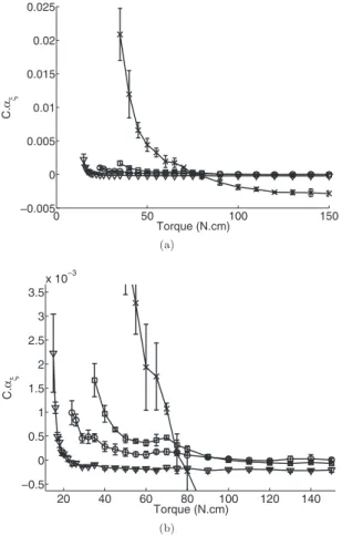
0 50 100 150 −0.01 0 0.01 0.02 0.03 0.04 0.05 Torque (N.cm) C. α f (a) 20 40 60 80 100 120 140 0 0.5 1 1.5 2 2.5 3 x 10⁻³ Torque (N.cm) C. αf (b)
FIG. 6.共a兲 Nonlinear elastic parameter C␣fas a function of torque for mode nos. 11共䉮兲, 20 共䊐兲, 21 共䊊兲, and 22 共⫻兲, where C is a constant. Mode No. 11 is present in the spectrum over the entire torque range, while modes 20, 21, and 22 appear at torque 35 N cm, 24 N cm, and 35 N cm, respectively. 共b兲 Zoom of 共a兲 on modes 11, 20, and 21.
eters. The behavior is highly similar, even if modal damping ratio共linear parameter兲 is more artifacted by the presence of adjacent modes.
Nonlinear parameters provide different information to the system, complementary to linear ones. This point will be developed more in-depth below.
A variation in nonlinear parameters is observed for most modes having a nodal line in the region of the screw, corre-sponding to a maximum strain. This maximum strain 共and
stress兲 at the interface acts as a probing of the threaded in-terface. Indeed, each bending oscillation will induce a rela-tive micromotion between the screw and the plate, revealing and describing the nonlinear nature of the contact. In con-trast, for modes with maximum displacement at the screw 共corresponding to a zero strain兲, the plate and screw move together without 共or with weak兲 relative micromotion, lead-ing to small values␣, and independent of the torque level. However, some exceptions are noted. Indeed, mode no. 6 or 8 共around 9 kHz兲 present a similar nodal line but their pa-rameters ␣ remain independent of torque. We do not fully understand this observation but we speculate that these pa-rameters may be dependent at torques lower than 15 N cm. Sensitivity results are summed up in the TableII.
V. DISCUSSION
The primary purpose of this study was to show that non-linear resonance spectroscopy was a useful tool to probe a threaded interface. In an applied aim, we show that this non-linear method provide a sensitive parameter␣. A comparison is made between linear and nonlinear parameters. We note they they measure different physical characteristics. The lin-ear measures are of complex moduli and density fluctuation; nonlinearity is a measure of material and interface integrity. It appears that nonlinear parameters are sensitive over a nar-rower torque range but are more sensitive than linear param-eters in this range. Furthermore, by following several modes in the spectrum and by analyzing modes which are not present in the entire torque range, we are able to increase the sensitivity range of the nonlinear approach. This could be implemented in a future as a “nonlinear modal analysis.” In terms of basic research this study constitutes one of the first combining nonlinear acoustic methods with threaded inter-face. Other nonlinear methods 共including frequency mixing and slow dynamics experiments兲 may be tested in the future as well. Both academic and application ways will be dis-cussed in the following subsections.
A. Physical modeling and nonlinearity origins
For the lowest torques共Fig.5兲, the evolution of the rela-tive frequency shift and damping variation in mode no. 11
0 50 100 150 −0.005 0 0.005 0.01 0.015 0.02 0.025 Torque (N.cm) C .αξ (a) 20 40 60 80 100 120 140 −0.5 0 0.5 1 1.5 2 2.5 3 3.5 x 10⁻³ Torque (N.cm) C. αξ (b)
FIG. 7.共a兲 Nonlinear dissipative parameter C␣as a function of torque for mode nos. 11共䉮兲, 20 共䊐兲, 21 共䊊兲, and 22 共⫻兲, where C is a constant. Mode No. 11 is present in the spectrum over the entire torque range, while modes 20, 21, and 22 appear at torque 35 N cm, 24 N cm, and 35 N cm, respec-tively.共b兲 Zoom of 共a兲 on modes 11, 20, and 21.
−16 −14 −12 −10 −8 −6 −4 −2 0 x 10−4 −C αf 20 40 60 80 100 120 140 13.945 13.95 13.955 13.96 13.965 13.97 13.975 13.98 13.985 f0 (kHz) Torque (N.cm) f0 −Cαf
FIG. 8. Mode No. 11. Evolution of linear共f0in dashed line兲 and nonlinear 共−C␣fin bold line兲 elastic parameters vs torque. The opposite value of C␣f is plotted to allow the sensitivity comparison.
0 50 100 150 0 20 40 60 80 100 Torque (N.cm) N orma lize d va lues
FIG. 9. Normalized values from 0 to 100 for linear共f0in dashed line兲 and
nonlinear共−C␣f in bold line兲 elastic parameters of mode nos. 11 共䉮兲, 20 共䊐兲, 21 共䊊兲, and 22 共⫻兲. The opposite value of C␣fis plotted to allow the sensitivity comparison.
does not seem to be linear but rather quadratic. Thus, by fitting a second order polynomial on these curves, it appears that a combination of␦ and␣ 共cubic and hysteretic nonlin-earities, respectively兲 is more appropriate, reflecting the co-existence of classical and hysteretic regimes simultaneously. Nevertheless, a coarse linear fit allows to compare a same parameter over the entire torque range.
Furthermore, this study points out a need for a model to characterize the nonlinear behavior of a threaded interaction under acoustic wave excitation, and beyond the PM space formalism presented in part II. The nonlinear behavior of the system comes from the interface between the screw and the plate. Indeed, and similarly to rocks where grains共rigid sys-tem兲 are interconnected with softer bondings, the interface screw/plate can be considered as a soft object between two rigid objects共screw and plate themselves兲. The nonlinearity level will depend on static forces present at the interface, the roughness of both surfaces, the presence of a liquid, etc.
This model will have to describe共1兲 the coexistence of classical and hysteretic regimes at lower torques and 共2兲 a decrease in both nonlinear parameters with increasing torque until the linear regime, with a faster decrease for the classical parameter.
As a starting point, asperities at the interface are usually modeled as microspheres in contact, and described by a Hert-zian nonlinearity. Indeed, this model can describe the pres-ence of classical regime at low torques. This model allows to describe the contact between two unconsolidated spheres un-der normal forces, giving a classical nonlinear elasticity.51 Then, models derived from the Hertz–Mindlin theory take
into account both normal and tangential forces and the pos-sibility of a stick/slip behavior. The latter leads to a hyster-etic regime52 and could be efficient to describe a threaded interaction at higher torques. From these previous consider-ations, we speculate that the ratio “interface area without stick/slip behavior” over “interface area with stick/slip be-havior” could be higher at low torque, corresponding to the evolution from the classical regime to the hysteretic one.
In Figs.6, 7, and 9, we observe that ␣f and␣ remain constant or slightly increase for increasing torques around 65–70 N cm, and for three modes 共20, 21, and 22兲. This behavior was not expected but does not seem an artifact as it is present for three different modes. One hypothesis that can explain this plateau is that the increasing prestress at the interface共i.e., increasing torque兲 could be separated in three different regimes. A first one at low torque where both sur-faces are only partially in contact, leading to weak contacts at the interface and high nonlinearity level, a second regime at high torque where nonlinearity is near zero, reflecting the fact that both surfaces are in contact, with all asperities squeezed at the interface, and an intermediate regime at mid-torque where both surfaces are in contact with asperities not all squeezed and leading to intermediate nonlinearity levels. Finally, the plateau observed at mid-torque could be ex-plained by the fact that asperities, not yet in contact in the first regime, could produce a second nonlinearity source, by friction and/or clapping, at a scale共micrometer or less兲 lower than in the first regime. This hypothesis, if verified by future experiments, could be of a potential interest as the linear
TABLE II. Summary of results obtained for each mode. Torque range of sensitivity for␣fand␣are displayed, as well as the presence of a nodal line of
displacement on the screw共corresponding to a maximum strain兲.
Number
Frequency 共Hz兲
Torque range of existence 共N cm兲 Torque range of sensitivity for␣f 共N cm兲 Torque range of sensitivity for␣ 共N cm兲 Nodal line on the bolt
1 1846 15–150 Very weak Very weak No
2 3447 15–150 Very weak Very weak No
3 4665 15–150 Very weak Very weak No
4 4832 15–150 Very weak Very weak Yes
5 8140 15–150 Very weak Very weak No
6 8373 15–150 Very weak Very weak Yes
7 8567 15–150 Very weak Very weak No
8 9369 15–150 Very weak Very weak Yes
9 10 330 15–150 Very weak Very weak No
10 13 800 15–150 Very weak Very weak No
11 14 010 15–150 15–40 15–30 Yes
12 15 600 15–150 15–40 15–40 Yes
13 16 040 15–150 Very weak Very weak No
14 17 300 15–150 Very weak Very weak No
15 17 450 15–150 15–40 15–40 Yes
16 Not excited
17 19 120 15–150 Overlapping with 18 Overlapping with 18 Not detected
18 19 380 15–150 Overlapping with 17 Overlapping with 17 No
19 Not excited
20 20 790 35–150 35–120 35–120 Yes
21 21 460 24–150 24–120 24–120 Yes
corresponding parameters are not influenced during this pla-teau 共see Fig. 9, f0 for modes 20, 21, and 22 increase for
increasing torques兲.
Finally, to model the entire sequence of phenomena de-scribed in part II 共for example slow dynamics effect, not studied here but evaluated in part III,共⬍5 s兲兲, we highlight three models that may be applicable. The first one, termed the “soft-ratchet model,”53 combines a nonlinear fast system of longitudinal resonance with a second slow system of ruptured/cohesive intergrain bonds. The fast sub-system includes a nonlinear stress-strain relation based on the Mie potential 共generally used in micromechanics to de-scribe intermolecular potentials54兲 to describe intergrain rela-tions in rocks. The slow one includes two activation param-eters, corresponding to bond rupture and restorations. The second model55 combines the PM space with thermally in-duced transitions to model conditioning and slow dynamics effects. Finally, the third one uses a Preisach–Arrhenius model, derived from the PM space, and which allows to include dispersion of linear and nonlinear acoustic properties taking account thermal fluctuations of the system.47In future work, we will apply one or more of these models to the system.
B. Multimodal measurement
This study constitutes one of the rare systematic nonlin-ear resonance spectroscopy applications in a multimodal context. Therefore, we remark on several points. Each mode have to be isolated from adjacent ones to avoid artifacts in the analysis, especially for dissipative parameters. Hence, modes at relatively low frequency are generally the most suitable, as the mode density is low. Moreover, the system geometry has to be as asymmetric as possible, to avoid sev-eral eigenmodes around the same frequency. We also observe that the most suitable configuration to perform a measure-ment occurs when emittor and detector are placed on a strain node 共or a maximum displacement兲, which favors an ener-getic mode, while the source of nonlinearity is placed on a displacement node 共or a maximum strain兲, which favors a sensitive mode. Also, when the source of nonlinearity re-mains unknown, sensitivity or insensitivity of different modes allows one to localize it.39
C. Strain level
The strain level applied by the acoustic wave to thread remains unknown共nonlinear parameter obtained is not␣but C␣, with a constant C兲. However, by using piezoelectric characteristics of sensors used in the experiment, we are able to obtain an order of magnitude for strain applied to the system. Indeed, strain applied to the emittor is between 10−6
and 5⫻10−5 for the lowest and highest amplitudes of
exci-tation, respectively, while the strain received by the detector is between 5⫻10−9 and 10−7. This evaluation does not give strain values received by the threaded interface but values of this order are speculated.
D. Measurement artifacts
We noted previously that for the highest torques, slopes are slightly negative in Fig.5共b兲, leading to negative␣ val-ues such as: they correspond to a transparency effect.56 Moreover, when performing the experiment without the screw in place, the nonlinear dissipative parameter is also slightly negative and with similar values. We do not find any physical reasons for this behavior and infer that it arises from electronic devices, bonding of piezoelectric sensors, and/or geometric nonlinearity.
VI. CONCLUSIONS
This is the first study presenting results of nonlinear resonance spectroscopy to a threaded interface, in a multi-modal way. Nonlinear parameters appear to be a useful tool to characterize this interface, complementary to linear ones. We also show that a multimodal study allows to increase the torque range of sensibility. Beyond the application interest, these measurements revealed some physical information on the interface, which can be mainly linked with friction theo-ries. For better comprehension, other nonlinear methods 共in-cluding frequency mixing and slow dynamics experiments兲 may be tested in the future to increase characterization. The study will be carried on in the future by both academic works and medical or industrial applications.
1F. R. Rollins, IEEE Trans. Sonics Ultrason. SU18, 46共1971兲. 2H. J. McFaul, Mater. Eval. 32, 244共1974兲.
3J. S. Heyman,Exp. Mech.17, 183共1977兲. 4J. F. Smith and J. D. Greiner, J. Met. 32, 34共1980兲.
5S. A. Nassar and A. B. Veeram, J. Pressure Vessel Technol.128, 427
共2006兲.
6S. Chaki, G. Corneloup, I. Lillamand, and H. Walaszek, Mater. Eval. 64,
629共2006兲.
7T. Zweschper, A. Dillenz, and G. Busse, Insight 43, 173共2001兲. 8T. Zweschper, A. Dillenz, and G. Busse,Proc. SPIE4360, 567共2001兲. 9M. Morozov, G. Rubinacci, A. Tamburrino, S. Ventre, and F. Villone, in
Electromagnetic Nondestructive Evaluation (IX), AIP Conf. Proc. No. 25
共AIP, New York, 2005兲, pp. 195–202.
10S. Paillard, G. Pichenot, M. Lambert, H. Voillaume, and N. Dominguez, in
Review of Progress in Quantitative Nondestructive Evaluation, AIP Conf.
Proc. No. 894共AIP, New York, 2007兲, pp. 265–272.
11Y. Le Diraison, P. Y. Joubert, and D. Placko,NDT Int.42, 133共2009兲. 12N. Raghu, V. Anandaraj, K. V. Kasiviswanathan, and P. Kalyanasundaram,
in Neutron and X-ray Scattering in Materials Science and Biology, AIP Conf. Proc. No. 989共AIP, New York, 2008兲, pp. 202–205.
13J. R. Tarpani, A. H. Shinohara, V. Swinka Filho, R. R. da Silva, and N. V.
Lacerda, Mater. Eval. 66, 1279共2008兲.
14M. Cacciola, Y. Deng, F. C. Morabito, L. Udpa, S. Udpa, and M. Versaci,
Int. J. Appl. Electromagn. Mech. 28, 297共2008兲.
15P. Y. Joubert and J. Pinassaud,Sens. Actuators, A129, 126共2006兲. 16N. Meredith, D. Alleyne, and P. Cawley,Clin. Oral Implants Res.7, 261
共1996兲.
17B. Dhoedt, D. Lukas, L. Muhlbradt, F. Scholz, W. Schulte, F. Quante, and
A. Topkaya, Dtsch. Zahnaerztl. Z. 40, 113共1985兲.
18A. Zagrai, D. Doyle, and B. Arritt, Proc. SPIE 6935, 93505共2008兲. 19D. Doyle, A. Zagrai, B. Arritt, and H. Cakan, Proceedings of ASME on
Smart Materials, Adaptive Structures and Intelligent Systems, 2009, Vol. 2, pp. 209–218.
20I. Solodov, K. Pfleiderer, H. Gerhard, S. Predak, and G. Busse,NDT Int. 39, 176共2006兲.
21P. A. Johnson, T. J. Shankland, R. J. Oconnell, and J. N. Albright, J.
Geophys. Res.,关Solid Earth Planets兴92, 3597共1987兲.
22P. A. Johnson, B. Zinszner, and P. N. J. Rasolofosaon,J. Geophys. Res.,
关Solid Earth兴101, 11553共1996兲.
23J. Y. Kim, L. J. Jacobs, J. Qu, and J. W. Littles,J. Acoust. Soc. Am.120,
1266共2006兲.
24K. Van Den Abeele and J. De Visscher,Cem. Concr. Res.30, 1453共2000兲. 25J. A. TenCate, Rev. Prog. Quant. Nondestr. Eval. 557, 1229共2001兲. 26C. Payan, V. Garnier, J. Moysan, and P. A. Johnson,J. Acoust. Soc. Am.
121, EL125共2007兲.
27V. Bucur and P. N. J. Rasolofosaon,Ultrasonics36, 813共1998兲. 28M. Muller, A. Sutin, R. Guyer, M. Talmant, P. Laugier, and P. A. Johnson,
J. Acoust. Soc. Am.118, 3946共2005兲.
29T. J. Ulrich, P. A. Johnson, M. Muller, D. Mitton, M. Talmant, and P.
Laugier,Appl. Phys. Lett.91, 213901共2007兲.
30W. L. Morris, O. Buck, and R. V. Inman,J. Appl. Phys.50, 6737共1979兲. 31I. Y. Solodov, A. F. Asainov, and S. L. Ko,Ultrasonics31, 91共1993兲. 32S. Biwa, S. Hiraiwa, and E. Matsumoto,Ultrasonics44, e1319共2006兲. 33K. E. A. Van den Abeele, P. A. Johnson, and A. Sutin, Res. Nondestruct.
Eval. 12, 17共2000兲.
34I. Solodov, J. Wackerl, K. Pfleiderer, and G. Busse,Appl. Phys. Lett.84,
5386共2004兲.
35V. Zaitsev, V. Gusev, and B. Castagnede, Phys. Rev. Lett.89, 105502
共2002兲.
36B. Mi, J. E. Michaels, and T. E. Michaels,J. Acoust. Soc. Am.119, 74
共2006兲.
37G. Renaud, S. Calle, and M. Defontaine, Appl. Phys. Lett.94, 011905
共2009兲.
38K. E. A. Van den Abeele, J. Carmeliet, J. A. Ten Cate, and P. A. Johnson,
Res. Nondestruct. Eval. 12, 31共2000兲.
39K. Van Den Abeele,J. Acoust. Soc. Am.122, 73共2007兲.
40L. D. Landau and E. M. Lifshitz, Theory of Elasticity, Theoretical Physics
Vol. 7, 3rd ed.共Butterworth-Heinemann, Oxford, 1986兲.
41J. A. TenCate, D. Pasqualini, S. Habib, K. Heitmann, D. Higdon, and P. A.
Johnson,Phys. Rev. Lett.93, 065501共2004兲.
42D. Pasqualini, K. Heitmann, J. A. TenCate, S. Habib, D. Higdon, and P. A.
Johnson,J. Geophys. Res.112, B01204共2007兲.
43L. K. Zarembo and V. A. Krasil’nikov,Sov. Phys. Usp.13, 778共1971兲. 44L. A. Ostrovsky, I. A. Soustova, and A. M. Sutin, Acustica 39, 298共1978兲. 45J. A. Ten Cate and T. J. Shankland,Geophys. Res. Lett.23, 3019共1996兲. 46R. A. Guyer, K. R. McCall, and K. Van Den Abeele,Geophys. Res. Lett.
25, 1585共1998兲.
47V. Gusev and V. Tournat,Phys. Rev. B72, 054104共2005兲.
48R. A. Guyer, K. R. McCall, and G. N. Boitnott,Phys. Rev. Lett.74, 3491
共1995兲.
49R. A. Guyer and P. A. Johnson, Nonlinear Mesoscopic Elasticity: The
Complex Behaviour of Rocks, Soil, Concrete 共Wiley-VCH, Weinheim,
2009兲.
50P. Johnson and A. Sutin,J. Acoust. Soc. Am.117, 124共2005兲. 51L. Ostrovsky and P. A. Johnson, Riv. Nuovo Cimento 24, 1共2001兲. 52V. Aleshin and K. Van Den Abeele,J. Mech. Phys. Solids57, 657共2009兲. 53O. O. Vakhnenko, V. O. Vakhnenko, and T. J. Shankland,Phys. Rev. B71,
174103共2005兲.
54H. Y. Erbil, Surface Chemistry of Solid and Liquid Interfaces共Wiley, New
York, 2006兲.
55P. P. Delsanto and M. Scalerandi,Phys. Rev. B68, 064107共2003兲. 56V. Gusev and V. Y. Zaitsev,Phys. Lett. A314, 117共2003兲.