HAL Id: hal-00358771
https://hal.archives-ouvertes.fr/hal-00358771v2
Submitted on 15 Jul 2010
HAL is a multi-disciplinary open access
archive for the deposit and dissemination of
sci-entific research documents, whether they are
pub-lished or not. The documents may come from
teaching and research institutions in France or
abroad, or from public or private research centers.
L’archive ouverte pluridisciplinaire HAL, est
destinée au dépôt et à la diffusion de documents
scientifiques de niveau recherche, publiés ou non,
émanant des établissements d’enseignement et de
recherche français ou étrangers, des laboratoires
publics ou privés.
The Gaia Mission and the Asteroids. A perspective
from space astrometry and photometry for asteroids
studies and science.
D. Hestroffer, Aldo Dell’Oro, Alberto Cellino, Paolo Tanga
To cite this version:
D. Hestroffer, Aldo Dell’Oro, Alberto Cellino, Paolo Tanga. The Gaia Mission and the Asteroids. A
perspective from space astrometry and photometry for asteroids studies and science.. Souchay, Jean
J.; Dvorak, Rudolf. Dynamics of Small Solar System Bodies and Exoplanets, Springer, pp.251-340,
2010, Lecture Notes in Physics, �10.1007/978-3-642-04458-86�. �hal-00358771v2�
A perspective from space astrometry and photometry
for asteroids studies and science.
Daniel Hestroffer1, Aldo dell’Oro2,1, Alberto Cellino2, Paolo Tanga3
1
IMCCE, CNRS, Observatoire de Paris, 77 avenue Denfert Rochereau, 75014, Paris, France
e-mail:hestroffer@imcce.fr
2 INAF-Osservatorio Astronomico di Torino, strada Osservatorio 20, 10025 Pino
Torinese, Italy
e-mail: delloro@oato.inaf.it, cellino@oato.inaf.it
3
Cassiop´ee, CNRS, Observatoire de la Cˆote d’Azur, France
e-mail: Paolo.Tanga@oca.eu
Summary. The Gaia space mission to be operated in early 2012 by the European Space Agency (ESA), will make a huge step in our knowledge of the Sun’s neighbor-hood, up to the Magellanic clouds. Somewhat closer, Gaia will also provide major improvements in the science of asteroids, and more generally to our Solar System, either directly or indirectly. Gaia is a scanning survey telescope aimed to perform high accuracy astrometry and photometry. More specifically it will provide physical and dynamical characterization of asteroids, a better knowledge of the solar system composition, formation and evolution, local test of the general relativity, and link-ing the dynamical reference frame to the kinematical ICRS. We develop here the general aspects of asteroid observations and the scientific harvest in perspective of what was achieved in the pre-Gaia era. In this lecture we focus on the determination of size of asteroids, shape and rotation, taxonomy, orbits and their improvements with historical highlight, and also the dynamical model in general.
Key words: Gaia ; astrometry ; photometry ; asteroid physical properties ; dy-namic ; orbit determination
In memoriam of Jacques Henrard (1940–2008). We dedicate this article to this wonderful colleague from the FUNDP (Namur), who was—as long as possible—an assiduous participant to such winter schools of the CNRS, and did always share his bright mind and high excitement in science and research.
Foreword
This paper is a compulsion of several of this CNRS school courses given in Bad-Hofgastein completed by some additional material. It is not intended to give a complete review of the Gaia capabilities for asteroids science, or of the treatment of orbit determination and improvement since the beginning of orbit computation. Neither will it cover each of the different techniques used for any particular problem. We hope however that it gives an overview of the Gaia mission concept, astrome-try and photomeastrome-try of asteroids (and small bodies) in particular from space, and current developments in this research topic. Besides, this school being in French in a German speaking place, some French and German bibliography have sometime been favoured or added.
1 Introduction
Before entering into the description of the Gaia mission observations and the dis-cussion of the expected results for asteroids science, we will briefly remind the basic principles from the Hipparcos mission, and then give an overview of the Gaia
objectives ($2). We will present the Gaia satellite and instruments as well as its
operational mode ($3), and expected scientific results for the Solar System ($4). In
the next sections we will develop more specifically three aspects: the astrometric CCD signal yielding the fundamental astrometric position and marginal imaging
capabilities ($5), the photometric measure yielding physical properties of asteroids
($6) and the dynamical model from the asteroids astrometry ($8). This provides a
solid overview of what can be achieved in the domain of planetology and dynamical planetology of asteroids. The following sections are more general and not exclusively related to Gaia. There we develop the general problem of orbit determination and
improvement for the case of asteroids orbiting around the Sun ($9), we give a short
description of both historical and modern methods. Finally we treat the case of
or-bit determinations of binaries ($10) focusing mainly on resolved binaries. But since
the problem of orbit reconstruction for extra-planetary systems appeared to be of importance for this school it has been briefly addressed here through the problem of
astrometric binaries ($10.4). Extra-solar planets is another topic actually addressed
by Gaia, but this is out of the Solar system, and out the topic of the present lecture.
2 Gaia – The context
2.1 Before Gaia – The Hipparcos legacy
Ten years have passed now since the publication of the Hipparcos catalogue in 1997. This space mission did provide a scientific harvest in many fields of
astron-omy and even, indirectly, in Earth science [85]. The Hipparcos mission provided
a homogeneous astrometric catalogue of stars with more sources and more precise
than were the Fundamental Katalog series during the 20th century. The acronym
“HIgh Precision Parallax COllecting Satellite” –in honour of the Greek astronomer Hipparchus—recalls that the basic output is of course the measure of the parallax of
stars and their proper motions. In fact there were two programmes or instruments on board the satellite: Hipparcos and Tycho. Both provide astrometry and pho-tometry of the celestial sources that were observed over the period 1989-1993, and two catalogues of stars were derived as well, the Hipparcos and Tycho catalogues. The Tycho data is based on the “sky mapper” which gives the detection of sources and triggers the main astrometric field observations for Hipparcos. It is hence less precise than Hipparcos but has more targets (about 2,500,000 stars in its version second version Tycho2 in the year 2000) than Hipparcos (about 120,000), and pro-vides two-dimensional astrometry as well as photometry in two bands close to the
Johnson B and V. Additional treatment of the raw data has been undertaken [117].
Further details on the Hipparcos/Tycho mission and instrumentation can be found
in e.g. [57,58] in the context of high accuracy global astrometry, and [43,47,84, Vol.
1, Sec. 2.7] for all details on the solar system objects observations and catalogues. The Hipparcos and Tycho Solar System Annex files (solar ha, solar hp,solar t)
are available on the CDS data-base4. While Hipparcos and Tycho were designed to
observe stars, they nevertheless could also provide data for solar system objects: 48
asteroids, 5 planetary satellites and 2 major planets5. There were different limiting
factors depending on the programme instrumentation: for Hipparcos, magnitude brighter than V ≤ 12.4 and size smaller than φ ≤ 1 arcsec, for Tycho magnitude brighter than V ≤ 12 and size smaller than φ ≤ 4 arcsec. But the more stringent one was that Hipparcos could only observe a very limited number of objects in its field of view (FOV), both for stars or asteroids.
The basic principle of the mission was to derive relative positions of targets observed simultaneously in two well separated fields of view. The measure principle consists basically in observing the target while it crosses the field of view with a photometer and to record the photon flux as modulated by a periodic grid. In ad-dition to the relative astrometry given by the grid, the photometers also recorded
the total flux, providing the magnitudes in the broad Hp ≈ VJ+ 0.3035 (B − V )
system for Hipparcos, and in two (red and blue) bands for Tycho. The Tycho astro-metric and photoastro-metric data are less precise than their Hipparcos counterpart, and concern only 6 asteroids compared to 48 asteroids observed within the Hipparcos mission.
The Hipparcos measure of position and magnitude of these selected solar system objects provided many scientific outcomes. We list a few showing the diversity of the applications:
- From the observed positions of the satellites, and taking one model for their ephemerides, one can derive the (pseudo-)position of the system barycenter, and/or the center of mass of the planet, as well. Such positions are model dependant since one uses the theory for the orbits of the satellites, but they
are far more precise than direct observations of the planets themselves [73].
- The particular photometry derived by one of the data reduction consortium (FAST) comprises the classical apparent magnitude together with an addi-tional one that is biased for non point-like sources. This allowed to indirectly
resolve the object and derive information on its size and light distribution [46].
4
URL: http://webviz.u-strasbg.fr/viz-bin/VizieR?-source=I/239/
5
Pluto was not observed which spare us the trouble of having to name this object observed in the past, before last IAU resolution.
- Hipparcos astrometry enabled the determination of the mass of (20) Massalia
from a close encounter with the asteroid (44) Nysa [4].
- High accuracy astrometry of asteroids enabled to improve their ephemerides [50],
and also to detect small systematic effects due to the photocentre offset[44].
- High accuracy astrometry of asteroids enables to link the dynamical inertial frame
to the catalogue [101,5,22].
- The stellar astrometric catalogue, mostly Tycho2, has an indirect consequence on science for the Solar System. Such stars provide better astrometric reductions for modern CCD observations of solar system objects, as well as re-reduction for older plates (the problem is still the low density when compared to e.g. UCAC2); they also provide much better predictions for stellar occultation path
[26,102,28].
Compared to Gaia observation and science of solar system objects, Hipparcos was most a (nice) prototype, or a precursor. They still have many common points:
- obviously space-based telescopes are exempt from all many atmosphere-related
problems (seeing, refraction, ...) and provide better stability (mechanical ther-mal) and a better sky coverage (not limited to one hemisphere);
- scanning law with a slowly precessing spin axis (going down to solar elongations
≈ 45◦);
- simultaneous observation of two fields of view for global astrometry;
- astrometric and photometric measurement, the colour-photometry being
manda-tory for correction to the astrometry.
The main difference between the two missions arise from the use of CCD device for Gaia instead of a photo-multiplier channel with Hipparcos/Tycho, and to a lesser extent the capabilities of onboard data-storage as well as data transmission to the ground-segment. Albeit CCD observations were already in use in astronomy and astrometry in particular during the 80’s, Hipparcos could not benefit of this technique: CCDs were still not validated for use in space (which requires a higher quality and robustness) and in any case the design of the satellite had to be set long before the beginning of the mission (often satellites are launched with out-dated material). The consequences are dramatic in terms of number of celestial bodies observable and general astrometric and photometric accuracy: Gaia is not an Hipparcos-II. The limiting magnitude of Tycho was V ≤ 12, but the catalogue
is far from being complete6 at that level; in comparison the limiting magnitude of
Gaia will be V ≤ 20. The border of Hipparcos is at 200 kpc, while Gaia will reach a large part of the Milky Way up to the Magellanic clouds.
In this respect also Gaia is different from the SIM mission [98,99] (USA) which
will provide very accurate parallax but for a very limited number of targets. The smaller Japanese mission Jasmine has more common points but, observing in the infra-red, the scientific goals are orthogonal and complementary. Last, the two Eu-ropean satellites differ in their location in space, Hipparcos missed its geostationary orbit and was on an eccentric one, Gaia will be at the L2 Sun-Earth Lagrangian point. Gaia will also observe a large number of solar system objects (mainly aster-oids) which data will provide new insights and scientific results as developed in the next sections.
6
Hipparcos with its larger-band filter can reach slightly fainter magnitudes, 12.5, but is anyway much less complete than Tycho.
Fig. 1. The Hipparcos (left) and Gaia (right) satellites in a pictorial view. Hip-parcos: one sees above the thruster and solar arrays one of the telescope baffle, for one of the observing direction. Gaia: the large, circular sunscreen will be deployed after launch and cargo to L2, it protects the instruments and permit their thermal stability. The telescopes, detectors and associated circuitry are situated inside the hexagonal or cylindrical housing.
2.2 What is Gaia?
The Gaia mission was designed to provide a renewed insight in the Galaxy structure, through a homogeneous set of very accurate measurements of stellar positions,
motions and physical properties [69, ?]. However, the independence from any input
catalogue grants that a very large number of non-stellar sources will be additionally observed. In fact, Gaia will automatically select observable sources with a criteria mainly based on a single parameter, the magnitude threshold (V < 20).
During the preliminary study of the mission, the community of planetologists realised that the observations of asteroids by Gaia may have a strong scientific impact, allowing a general improvement of our view of the Solar System of the same order as in the case for stars [?]. Of course, the reasons are similar and are built on the unprecedented astrometric accuracy of Gaia and on its spectro-photometric capabilities.
One will note, however, that the strongest quality of the Gaia data—beside accuracy—will reside in homogeneity. In fact, no other single survey have produced an equivalent wealth of data for 300,000 Solar System objects, as is expected for
Gaia [70]. As we will illustrate in the following, a complete characterisation of the small bodies of the Solar System will be possible.
We can also compare Gaia to other forthcoming deep surveys, such as the very
important Pan-starrs7, expected to map the whole observable sky 3 times per
month at greater depth (V∼24, for the single observation at SNR=5). In this case, even more objects will be detected, and this will constitute a serious advantage to feed investigations of smaller or more distant and fainter asteroids. However, the astrometric and photometric accuracy—despite being optimised—will remain limited by ground-based conditions, and spectro-photometry will not be of the same level as in the case of Gaia. Other typical observational constraints for ground-based investigations also apply to Pan-starrs, including the minimum Sun elongation that will be reached, severely limiting its capabilities for the investigation of peculiar asteroid categories, like Earth crossers or the Inner Earth Objects. Last the sky coverage is limited to one hemisphere and global astrometry is hardly achieved with such systems (on the other hand they will benefit of the Gaia catalogue of stars).
For these reasons, and despite the limitation in brightness to V∼20, we believe that Gaia is rather unique and really has the potential to have a major impact in Solar System science. In this lecture, we will try to focus on the kind of data that the mission will provide, and on the corresponding data treatment that is being conceived in order to extract the relevant information. Hopefully, the observer will appreciate the techniques allowing to reach an exceptional accuracy, and the theoretician will find interesting new problems that must be solved to fully exploit the data scientific content.
3 The Gaia mission
3.1 Launch and orbitThe Gaia satellite will fit into the payload bay of a Soyuz fregat vector, that will be launched from the European base of Kourou (French Guyana). After a ∼1-month travel, it will reach the L2 Lagrangian equilibrium point, that is situated 1,5 million km from Earth, opposite to the Sun. The satellite will then deploy the solar panels, fixed on a large, circular sunscreen (diameter: 10 m) that lies on a
plane perpendicular to the spin axis (Fig.1). The visibility of the satellite and the
data link are reduced when compared to a geostationary orbit, but the environment is quieter. The L2 point is a dynamically unstable equilibrium location, requiring firing the satellite thrusters to apply trajectory corrections every ∼1 month. Gaia will thus be maintained on a Lissajous orbit around L2, allowing it to avoid eclipses of the Sun in the Earth shadow. The location thus appears as an optimal choice for constant sunlight exposure, and for maximum thermal stability. The planned operational lifetime of the mission will be 5 years.
3.2 The spacecraft
The beating heart of the satellite is enclosed in an approximately cylindrical struc-ture, including all the relevant parts: the thrusters openings and their fuel tanks,
the electronic equipment, and of course the optical train. Since we are interested in the observations, we will just give some fundamental design principles concerning the latter component [?].
The optical bench structure is based on an octagonal toroid built in silicon car-bide. This is a critical component, supporting all the optics and the focal plane. The measurement principle—being similar to that of Hipparcos—requires two different lines of sight, materialised by two Cassegrain telescopes. The primary mirrors are
rectangular and measure 1.45×0.50 m2. Five additional mirrors are required to fold
the optical path, obtaining an equivalent focal length of 30 m. The light beams are combined and focused on a single focal plane, composed by a matrix of 106 CCDs. The extreme rigidity of the toroidal structure (actively monitored during the mission) ensures that the angle between the two telescopes (also called “basic angle”) remains constant at 106.5 degrees.
The CCD array constitutes a large, 1-Gpixel camera, that can be compared (in pixel number) to the Pan-starrs cameras. However, it remains unrivalled in surface, since it extends over 0.93×0.46 m, by far the largest CCD array ever con-ceived.
The resolution anisotropy due to the rectangular entrance pupil of the tele-scopes are matched by strongly elongated pixels, about three times larger along the direction in which the diffraction spot is more spread.
Fig. 2. The focal plane receives the light beams of both telescopes. While spinning, Gaia scans the sky in such a way that images of sources enter the focal plane from the left and cross it moving toward the right. The whole crossing takes about 1 minute. Each CCD is crossed in 3.3 seconds. See the text for instrument details. The Basic Angle Monitoring (BAM) and Wave-front Sensor (WFS) CCDs are used for monitoring tasks.
The general organisation of the focal plane is illustrated in Fig. 2. Different
groups of CCDs are identified depending upon their functions, since they correspond in all respects to different instruments. The main Gaia instrument is the Astrometric Field (AF), receiving unfiltered light, which is devoted to produce ultra-precise
astrometry of the sources [?]. The other instruments are aimed at achieving spectral characterisation. The figure shows the Red and Blue Photometers (RP and BP), which will be receiving light dispersed by a prism, and have optimised sensitivity in two different, contiguous portions of the visible spectrum. The resolution of RP and BP is rather low, each portion being spread on ∼30 pixels. The Radial Velocity Spectrograph (RVS), on the other hand, provides a spectrum in a restricted wavelength range (847 − 874 nm) but with much higher resolution. It is aimed at sampling some significant spectral lines that can be diagnostic of stellar composition
and can be used to derive radial velocities with a ∼ 1 km.s−1 typical uncertainty.
Due to star crowding (superposition of spectra) and SNR constraints, RVS will have a limit magnitude at V = 17. This instrument will provide no scientific information for asteroids. On another hand the measures for the bright asteroids will be used to calibrate the kinematic zero point of the RVS, as a complement to the data from IAU standard stars.
Since Gaia is continuously spinning with a rotation period of 6 hours, the sources
will drift on the focal plane, entering from the left in the scheme of Fig. 2 and
travelling toward the right. The displacement will be compensated by a continuous drift of the photoelectrons on the CCD at the same speed; this technique (also used on fixed ground-based telescopes) is known as “TDI mode” (from “Time Delay Integration”). The resulting integration time (3.3 seconds) corresponds to the time interval required by a source to cross each CCD. Of course, this principle applies to all instruments. As a consequence, while an image of the source drifts on the AF CCDs, it will take the form of a dispersed spectra while moving on RP, BP and RVS.
An important part of the focal plane, the Sky Mapper (SM), requires some additional explanation. In fact, Gaia will neither record nor transmit to the ground reading values for all the pixels, due to constraints on the data volume. Conversely, only a reduced number of values ( “samples”), representing the signal in the imme-diate surroundings (“window”) of each source, will be processed and transmitted, and only for objects brighter than V = 20. These samples represent either the value of single pixels, or of some binning of couples of pixels, depending upon the star brightness. For stars with V > 16 (i.e., the largest fraction of sources) only 6 samples will be available, corresponding to the signal binned along 6 pixel rows in the direction perpendicular to the scan motion. These samples will be transmitted for each CCD in the AF field. Larger samples are required to accommodate the dispersion of RP, BP and RVS spectra.
As a consequence, the AF information on positions will be essentially one-dimensional, being very precise along the scanning circle, but very approximate in the across-scan direction. One should also note that the windows are assigned by the on-board algorithm after SM detection. Beside a confirmation of detection that is expected from the first AF column, no other controls are executed all along the focal plane crossing, and the window follows the object on each CCD, assuming that it shifts at the nominal scanning speed. While this is true for stars, we will see that Solar System objects will suffer measurement losses due to their apparent motion.
3.3 Observation principles: the scanning law
The accuracy requirements of the mission can be reached only if the sky coverage is fairly uniform. To obtain this result, the direction of the spin axis of the probe cannot obviously stay fixed, but it must change, slowly but continuously, to change correspondingly the orientation of the scanning circle on the sky.
Two additional rotational motions are thus added to the 4- revolutions-per-day
satellite spin (Fig.3). The first one is a precession of the spin axis in 70 days, along
Fig. 3. The Gaia scanning law, composed by three rotations (spin, precession and orbital revolution) as explained in the text.
a cone whose axis points towards the Sun. The change in orientation of the latter, provided by the orbital revolution around the Sun in 1 year, is the last additional rotation.
The overall motion, beside being derived from the scanning law optimisation, is also compatible with the need of keeping the system in thermal stability, since the incidence angle of the Sun light on the solar screens remains constant, and the enclosure of the scientific instruments is always consistently shadowed.
The scanning law that results from the combination of the three rotations per-mits 60 − 100 observations of any direction on the sky. Each one occurs with differ-ent oridiffer-entations of the scan circle, allowing to reconstruct the full two dimensional
position of fixed sources from positional measurements that are essentially one-dimensional.
The availability of the observations in two simultaneous directions, and their multiplicity, has an important consequence: the star measurements contain both the information needed to map their position on the sky, and that needed to reconstruct the orientation of the probe at any epoch. For this reason, the process of astrometric data reduction—the so called “Global iterative solution”—is an inversion procedure allowing to retrieve at the same time the parameters that define star positions, their proper motion and the attitude of the probe. The applicability and performances of this strategy have been fully proved in the previous Hipparcos mission.
4 Solar System science
While scanning the sky, sources corresponding to Solar System objects (planets, dwarf planets, asteroids, comets, natural satellites, ...) will enter the Gaia field of view, and will be detected and recorded. The main difference with respect to stars will come from their motion. Their displacement on the sky have two main consequences: they will not be re-observed at the same position; their motion will not be negligible even during a single transit.
These two basic statements are sufficient to dictate the need of a special data treatment for these objects. Several specific problems can thus be identified at first order, deserving an appropriate data reduction chain; we cite here:
– image smearing during integration time;
– signal shape due to resolved size and/or shape;
– de-centering relative to CCD windows, or total loss during one transit;
– identification of new objects from detections at different epochs.
These issues are strictly related to the basic characteristics of the mission, but also other challenges are present when the science content to be extracted is considered. They will be discussed in the following sections.
A specific management activity for Solar System data reduction has been cre-ated in the frame of the DPAC (Data Processing and Analysis Consortium), as a part of the “Coordination Unit 4” devoted to process specific objects needing spe-cial treatment (double stars, exo-planet systems, extended objects, Solar System objects).
Following the most recent mission specifications, one can identify the categories of objects that will be really observed by Gaia. In fact, all sources that will appear larger than ∼ 200 milli-arcsecond (mas) will probably be discarded and have no window assigned. This selection automatically excludes from observations the major planets, some large satellites (such as the Galilean satellites of Jupiter, or Titan) and also the largest asteroids (or dwarf-planets) when closer to Earth (Ceres, Pallas, Vesta, in particular).
On the other hand, small planetary satellites very close to major planets will be accessible thanks to the low level of contamination from light scattered by the nearby planet. However, the vast majority of the observed objects will consist of asteroids of every category: mostly from the Main Belt, then small ones belonging to the Near Earth Object population, and some additional tens among Jupiter Tro-jans, Centaurs, and Trans-neptunians. Using the most recent survey data, we can
estimate a population of ∼ 300, 000 asteroids to be observable by Gaia, representing just 1/4000th of all the sources that Gaia will measure.
Each asteroid will be observed (by the AF) ∼ 60 − 80 times during the nominal mission operational lifetime of five years, although the number of detections can be much lower for Near Earth Objects, sensibly depending upon the geometry of the observation. On average, we can estimate that no less than 1 asteroid/sec will enter the Gaia astrometric instrument when the viewing direction is close to the ecliptic. Most asteroids will be known when Gaia will fly, so the discovery potential of Gaia remains low and does not constitute in itself a reason of special interest for the mission. One exception can probably be represented by specific object categories easily escaping most ground-based surveys, such as low elongation Inner Earth Objects.
In fact, the geometry of the observations relatively to the positions of the Sun and the Earth can be easily estimated since most of the Solar System objects orbit the Sun at very low ecliptic inclinations. It is thus straightforward to use the
Fig. 4. At any given position along Earth orbit, the sky not accessible to the Gaia scan motion is delimited by two cones centered around opposition and conjunction with the Sun. When projected on the ecliptic, the unobservable region appears as the two grey regions in this picture. The observable portion of the orbit of a NEA and an MBA is enhanced.
relevant angles to identify the regions of the ecliptic plane that can be visited by
the Gaia scanning circle. The result is shown in Fig. 4 where the dashed sectors
represent the viewing directions that are compatible with the scanning law. As one can see, Gaia will never observe neither at the opposition nor toward conjunction, but mostly around quadrature.
More precisely, while quadrature represents the average direction, it won’t be the most frequent one, since the intersection of the scan plane with the ecliptic spends most of the time preferentially close to the extremes of the accessible region.
The region at ∼45 degrees elongation from the Sun will thus be explored and could represent the most fruitful area for discovery purposes. Another poorly known population, not easily accessible from the ground, is the one represented by asteroid satellites. In fact, binaries larger than ∼120 mas will be seen as separate sources by Gaia, and today it is hard to estimate how many of them will be discovered.
However, we stress that the full physical and dynamical characterisation of known objects is the much more ambitious and rewarding goal that is expected from the Gaia mission. In fact, preliminary studies have shown that the precision of Gaia observations (both for photometry and astrometry) will be able to improve
by more than 2 orders of magnitude the quality of asteroids orbits [104], to derive
a mass from mutual perturbations for ∼150 asteroids [70], to derive for most of
them a shape and the rotational properties by lightcurve inversion [20], to measure
General Relativity PPN parameters [45], to directly measure asteroid sizes [?], to
constrain non-gravitational accelerations acting on Earth crossers [105]. We will
detail in the following the most relevant of these issues.
As a result, we can already guess today that Gaia will open new perspectives for a better understanding of the Solar System—of asteroids in particular—portraying in a self-consistent way both dynamical and physical properties. Subsequent studies will take profit of the situation, for example by rebuilding observational approaches that exploit better orbit and size and shape data (see e.g. the asteroid occultation
case [103]).
5 Analysis of the astrometric signals
5.1 IntroductionThe CCD signal of a minor body transiting in the field of view of Gaia is charac-terised by some features that make it different from the ideal signal produced by a fixed star, and for this reason it requires a special treatment with respect to the standard processing pipeline adopted for stars.
First, it is important to understand what we mean in this lecture when we speak of “fixed stars”. A fixed star is an ideal point-like source whose motion on the celestial sphere can be considered nil during the time taken by the source to make a transit across the Gaia field of view (FOV). In practical terms, the celestial objects that most closely fit the above definition are not stars, but distant quasars. It is obvious that the property of being a non-moving source refers to the celes-tial sphere and not to the Gaia focal plane, since the Gaia field of view continuously changes while the satellite makes its scan of great circles on the celestial sphere (as a first approximation). However, as we will see in the following discussion, it may be said that the apparent motion of a fixed star in the Gaia FOV is at least ap-proximately cancelled out by the adopted process of signal acquisition.
In general, a point-like source produces a photon flux distribution across the focal plane that, for a rectangular pupil like that of Gaia, is essentially the Fraun-hofer diffraction pattern corrected for the aberrations introduced by the instrument optics itself. It is not our intention to discuss here all the details of the optical con-figuration of Gaia, but it is necessary to point out at least a few basic concepts. First, the response of the instrument to the distribution of photons produced by a
point-like source is called Point Spread Function (PSF). The PSF is necessarily the starting point to develop any description of the astrometric performances expected from Gaia. More in particular, the diffraction pattern produced on the focal plane by a point-like source not moving across the field of view is known as the optical PSF. By “diffraction pattern” we mean the bi-dimensional spatial distribution of the incident photons on the focal plane per unit area per unit of time. This includes the aberrations introduced by the instrument optics, the transmittance of the in-strument, the response of the CCD detectors, and it depends also on the spectral distribution of the source. In particular, if we call “quasi mono-chromatic optical PSF” the optical PSF produced by a source for which the spectral distribution of its emitted radiation is limited to a very small interval of wavelengths, then we may define a poly-chromatic optical PSF as the average of different mono-chromatic optical PSFs, each one weighted according to the spectral distribution of the source. The situation is more complex if we consider the effects related to the actual area of the focal plane (that in the case of Gaia is quite large). Distortions introduced by the instrument aberrations depend on the position of the source in the field of view. Sources in different positions in the field of view produce PSFs centered in different locations in the focal plane. Then, PSFs detected in different points of the focal plane, even if produced by the same kind of source and spectral distribution, show different features.
Moreover, due to the fact that in the adopted Gaia instrument configuration the signals are detected by an array of distinct CCDs, each having a well defined quantum efficiency (QE) which is wavelength-dependent, it follows that the different spectral components of the PSF are detected with different efficiencies. For this reason, when we talk about the PSF, or in general the signal, of a generic source, it is more convenient and straightforward to refer to the number of photoelectrons produced by the CCD detectors per unit of time instead of the number of incident photons per unit time on the detector itself. In other terms, in the rest of this lecture we will call PSF the diffraction pattern including the effect of CCD quantum efficiency. It is worthwhile to point out that the QE of the CCDs in the Gaia astrometric focal plane is nominally the same for all of them, and that no additional filters are placed in front of them.
As a matter of fact, however, the PSF of fixed stars is even not observable in the sense explained above, due to two fundamental reasons. First of all, the spatial resolution of the detector is finite because so is the dimension of the CCD pixels. As a consequence, the detector does not give the number of photoelectrons generated in any arbitrary point of the CCD per unit area and unit time, but it gives the total (integrated) number of photoelectrons collected by each pixel during the integration time. In other terms, the optical PSF has to be integrated within the rectangular area of the pixel and within the duration of the integration time. The second reason why the optical PSF is not directly observable is that, due to the complex motion of the satellite which allows it to scan the celestial sphere, any source moves within the field of view during the time in which it produces photoelectrons in the focal plane (source transit in the Gaia FOV). As a consequence, the PSF moves on the focal plane. Accordingly, the PSF is collected by all pixels and CCDs on which the PSF itself transits. Due to the effect of the apparent motion of the source in the FOV, the detected PSF should be smeared along the path that the image follows on the focal plane. In order to avoid this very undesirable effect, a transfer of charges from
pixel to pixel towards the read-out register is done at the same velocity and along the same direction of the apparent image motion. This technique of read-out of the CCD is known as Time Delayed Integration (TDI) mode. In TDI, the generated photoelectrons “follow” the portions of the PSF that produced them. Ideally, if the motion of the charges followed exactly the same trajectory as that of the image in the focal plane and at the same continuous rate, the spatial distribution of the recorded photoelectrons would reproduce exactly the PSF. Unfortunately, this is not strictly true in practice, for the charge transfer is not a continuous process. What happens in practice is that the motion of the collected photoelectrons is produced by transferring all charges within one pixel into the adjacent one in the along-scan direction at regular time steps. The duration of the time step, indicated as the TDI period, is set in order to minimise the spread of the PSF due to the source motion. Nevertheless, the TDI mode cannot guarantee a perfect cancelation of the PSF smearing. The reason is that, even if the TDI period is kept constant and the charge transfer is done along the instantaneous scan direction, what happens is that the motion of the image is neither uniform nor aligned exactly in the along-scan direction. On one hand, this is simply due to the precession motion of the spin axis of the satellite, which is constantly changing the orientation of the along-scan direction. But even in the case that the motion of the image on the focal plane was perfectly uniform and exactly aligned with the along-scan direction, nevertheless the TDI mode could not correct completely the PSF smearing. The reason is that during each single TDI period the charges are not transferred, whereas the image moves and the signal is smeared. In this way, photons coming from the same point of the optical PSF may be collected by two different pixels. The final effect is that the PSF is broader and systematically displaced in the along-scan direction.
In principle, the TDI period should be equal to the along-scan dimension of the pixels divided by the image velocity. Non uniformity of the along-scan motion introduces further distortion due to deceleration and acceleration of the image with respect to the TDI mean motion.
The PSF including the finite size of the pixels and the effect of the TDI mode is called total or effective PSF. But the real signal is affected also by other sources of noise and distortion. First of all, the signal is produced by a stochastic process, corresponding to the random sequence of photon arrivals and photoelectron gen-eration. Then, the final number of charges collected in a given pixel is a random number, typically governed by the Poisson statistics. Moreover, the signal is dis-torted by the effect of cosmic rays on the CCD, affecting also the Charge Transfer Efficiency (CTE) from one pixel to another. Some studies point out that some pack-ets of charges can be entrapped and be released later without correlation with the regular TDI mode. All these effects introduce distortions of the final signal that are under investigation.
The treatment of the signals produced by Solar System objects (SSOs) is even more difficult than in the “simple” case of fixed stars described above. SSOs are differently from stars, in that they are characterized by a much faster apparent motion. When we say that SSOs move we intend that they display a motion with respect to the fixed stars. As a consequence, the trajectory of SSO images across the focal plane does not follow the same pattern of fixed stars in the same field of view and their motion is not properly corrected by the TDI mode.
SSOs have a residual velocity with respect to the apparent motion of a fixed star, and this residual velocity has components both on the along-scan and the across-scan direction. This fact has the consequence that their final signals are spread. Moreover, while we may expect that for fixed stars the time interval between the transit on a given CCD and the adjacent one in the along-scan direction is constant, being about equal to the number of pixels in the along-scan direction in a CCD multiplied by the TDI period, this is no longer valid for a SSO. The transit of a SSO image on a CCD is either delayed or anticipated with respect to that of stars, depending on the residual velocity.
Velocity is not the only one peculiar features of SSOs to be taken into account. Another effect is that these objects may appear in general, or very often, as extended sources. This means that the final signal is not simply due to the PSF as for the case of point-like stars, but each point of a SSO image produces an independent PSF, and the final signal is the sum of all these PSFs. This means that the signal of a SSO depends on the size, the shape and the brightness distribution of its image. For all the above reasons the analysis of the signals of SSOs requires a special treatment with respect to the simpler one used for fixed stars.
5.2 Signal computation
Let be x and y the coordinates of a cartesian system associated to the focal plane, having the x-axis set along the scan direction and directed as the movement of charges of the TDI mode. Let I(x, y) be the photoelectron distribution produced by the optical image of a non moving source, that is the number of photoelectrons generated per unit area and unit time around the point of coordinates (x, y). The function I(x, y) contains information about both the PSF photoelectron distribu-tion f (x, y) and the apparent brightness distribudistribu-tion of the observed object g(x, y). From a mathematical point of view, I is the convolution of f and g:
I(x, y) = Z Z
g(x0, y0)f (x − x0, y − y0) dx0dy0 (1)
For sake of brevity multiple integrals signs will be omitted in the following. Let now τ be the TDI period. The signal, that is the number of photoelectrons collected by a pixel whose centre has coordinates (α, β), during the interval of time τ , from a
source image with centre located at coordinates (xc, yc), is given by:
S(α, β) = Z Z Z I(x − xc, y − yc)Π “x − α ∆x ” Π„ y − β ∆y « Π„ t τ « dx dy dt (2)
where ∆x and ∆y are the along-scan and across-scan dimensions of the pixels, t is the time, and Π(u) is the gate function equal to 1 for −1/2 ≤ u ≤ 1/2 and zero otherwise.
If now we assume that the image source moves with constant velocity, so that:
xc= ˙xt + x0 yc= ˙yt + y0
S(α, β) = Z I(x − ˙xt − x0, y − ˙yt − y0)Π “x − α ∆x ” Π„ y − β ∆y « Π„ t τ « dx d dt (3) Two comments are necessary at this point. For fixed stars it is assumed that
∆x = ˙xτ , but for SSOs this is not the case in general. In particular, if vτ is the
mean transfer velocity of the charges, so that vτ = ∆x/τ , the relevant parameter for
SSOs is the residual along-scan velocity µ = ˙x−vτ. Second, at every time interval of
duration τ the charges in a pixel are moved to its immediate adjacent pixel. In this
process, α → α + ∆x, while at the same time xc→ xc+ (µ + vτ)τ = xc+ ∆x + µτ
and yc → yc+ ˙yτ . For fixed stars we have α − x0 = const., assuming an ideally
perfect clocking, then in this case the total number of electrons recorded during the integration time T is simply T /τ times the number obtained over one pixel. This is not true for SSOs, and the computation of the integral has to be done for the entire integration time. For sake of simplicity the computation can be done under the assumption that the optical PSF is locally constant, or in other words that we may use the same PSF over one whole CCD.
In practical terms, the preferred option to attack the problem of signal com-putation has been so far based on a different, numerical ray-tracing approach. Let us then come back to consider the incoming photons from the source, before they start to interact with the optical system to produce the recorded image. We may
imagine a coordinate system following the moving object and with origin in (xc, yc)
and axes parallel to the along and across-scan directions. In this reference system, the photons coming from the source would produce an image in an hypothetic de-tector, and the coordinates of a given point belonging to this (static) image would
be x0 and y0. Now, we can easily compute the corresponding coordinates (x, y) in
the moving Gaia focal plane of the the photons coming from the (x0, y0) point just
defined above. These are:
x = x0+ ˙xt + x0
y = y0+ ˙yt + y0 (4)
In the adopted method of image simulation, based on a Monte Carlo algorithm,
all the quantities x0, y0 and t are randomly generated. The time t is uniformly
generated between −T /2 and T /2 where T is the integration time, while x0, y0are
randomly generated according to a given surface luminosity distribution g(x, y) of the object (chosen a priori ), using a ray tracing algorithm which takes also into account an assumed light scattering law characterising the object’s surface. For the
details of the numerical algorithm of generation of the sampling positions x0and y0
see [?]. The number N of sampling points (x0, y0) depends on the magnitude of the
object and on instrument characteristics including the CCD quantum efficiency. In particular, we have that M = −2.5 log N + C, where M is the apparent magnitude and C is a suitable constant. At magnitude 12, corresponding to the saturation limit of the CCD in astrometric focal field, the number of collected photoelectrons are about one million. The nominal magnitude limit of detection is V ≈ 20 and
corresponds to about one thousand photoelectrons [83]; see also $5.4.
Of course, the above optical image, or in other words the (x, y) distribution of incoming photons from the observed object, is not yet the final recorded signal. We have still to take into account the fact that each photon incident on the optical system suffers an angular deviation δx and δy, respectively, in the along-scan and
across-scan direction due to the diffraction of the instrument aperture. The nu-merical model reproduces the instrument diffraction effect by generating δx and δy randomly, but according to a parent distribution given by the PSF of the system. In other words, the probability of a given deviation is proportional to the value of the PSF f (δx, δy) for this particular deviation. In order to obtain the real arrival position of a single photon on the focal plane we have then to add δx to x and δy to
y. Obviously all the quantities x0, y0, δx and δy are expressed with the same unit.
As mentioned in the previous section, the spreading of the recorded photoelec-trons in the along-scan direction on the focal plane due to the scanning motion of the satellite, is reduced by the Time Delayed Integration (TDI) read-out mode. For this reason we introduce a moving coordinate system (X, Y ) synchronised with the TDI charge transfer. Obviously Y = y because no TDI correction is performed in the across-scan direction. In this way, the “effective” position of the photoelectron inside the CCD image turns out to be:
X = θ(x0+ δx + ˙xt + x0, t)
Y = y0+ δy + ˙yt + y0 (5)
where θ is a special function accounting for the step by step TDI translation, and depending on time t explicitly, according to the phase of the TDI charge transfer. In practical terms, however, TDI blurring is included in the adopted PSF, so that the θ function reduces to a simple continuous translation (see [?] for details). In this case, we may simply write down the following:
X = x0+ δx + ˙xt + x0
Y = y0+ δy + ˙yt + y0 (6)
where ˙x and ˙y represent the residual velocity of the object with respect to the
TDI motion. For SSOs, this corresponds in practice to the apparent motion with respect to the fixed stars.
The final step of the numerical procedure is the allocation of the photoelectrons into the corresponding pixels. The Gaia CCD detectors have rectangular pixels with smaller side ∆X = ∆x in the along-scan direction, and larger side ∆Y = ∆y in the across-scan direction. Each pixel is labelled with integer indexes i and j and corresponds to the rectangular region defined by the points (X, Y ) such that:
Xi≤ X < Xi+ ∆X ; Xi= i∆X Yj≤ Y < Yj+ ∆Y ; Yj= j∆Y (7)
in this way the origin of the coordinates system coincides with the the left-hand, lowest corner of the pixel labelled as i = 0, j = 0.
In the astrometric focal plane of Gaia only a limited region of the CCD grid is actually read-out. This window is, again, a rectangular n × m one, with a number n of pixels in the along-scan direction and m pixels in the across-scan direction. In this way 0 ≤ i ≤ n − 1 and 0 ≤ j ≤ m − 1. Following the sampling scheme
proposed by [52], 12 × 12 pixels windows should be used for stars between 12 and
16 magnitude (in the G-band of Gaia), and 6 × 12 windows for stars between 16 and
20 magnitude. We indicate by Nij the number of photoelectrons in the i-th pixel
of the window in the along-scan direction and the j-th in the across-scan direction. It is important to note that in general the recorded signal is binned, that is the numbers of pixels in the across-scan direction are integrated (summed up), so that the final signal consists of the n numbers:
Ni= m−1
X
j=0
Nij 0 ≤ i ≤ n − 1 (8)
In the following, we will assume that CCD window is always binned, and what we call “signal” is actually given by the set of discrete photoelectron counts just defined above.
5.3 CCD processing
In general terms, we call “CCD processing” a sequence of numerical procedures
aiming at extracting from the recorded signal Niall possible information of interest.
In particular, in the case of SSOs, four parameters are of great importance: the position of the object, its angular size, its velocity and its apparent magnitude. Basically, both for stars and SSOs, the adopted method of determination of all the relevant parameters is based on a best-fit procedure.
It is assumed that a mathematical model of the signal is at disposal, or in other
terms that we are able to compute the numbers Ni for any set of values of the
unknown parameters. This computation can be done analytically or throughout numerical codes. In addition to a signal model, one has to decide a criterion of comparison between the computed (C) and the observed (O) signal, in order to minimising or maximising some target function expressing the mathematical dis-tance between C and O.
We note that, in principle, an alternative approach, based on a full reconstruc-tion of the image, could also be adopted. A number of refined techniques of image reconstruction have been actually developed in the literature in several situations. On the other hand, it seems that such kind of approach can hardly be applied with success to poorly sampled signals covering only a few pixels, like those from faint, nearly point-like sources detected by Gaia. For this reason, we focus on the approach based on the determination of a limited number of relevant unknown properties of the sources by means of a signal best-fit approach.
For sake of simplicity, in order to focus on a few fundamental concepts rather than on unnecessary technical details, let us limit now to a one-dimensional case. Let L be the model function used to fit the recorded signal. For a fixed star this reduces to the PSF integrated in the across-scan direction and convoluted with the Π function describing the shape of the pixel. This leads to derive the so-called Line Spread Function (LSF). For fixed stars, this depends only on the position c in pixels of the star and on its apparent magnitude, or, in other words, on the total number of collected photoelectrons. The signal is proportional to the flux and can be reproduced by translating the centre of the LSF into the star position. If we call L the LSF per unit of flux (that is, normalised to one collected photoelectron) the
expected number of photoelectrons in the pixel i, E(Ni), is given by:
E(Ni) = r2+ b + N L(i − c) (9)
where N is the total number of photoelectrons produced by the source, and r is the RMS readout Poisson noise in electrons. The term b is the contribution of the
background in electrons per sample. We assume that r2+ b is known with sufficient
If Ni is the number of electrons really collected in the sample i, a method
of estimation of the unknown parameters c and N , corresponding to the unknown photocentre position and apparent magnitude of the source, can be based on a max-imum likelihood criterion. More precisely, c and N are varied in order to maximise
the probability of collecting the observed counts Ni, assuming the signal model L.
For Poisson statistics this probability is given by the likelihood function:
f (c, N ) = m−1 Y i=0 [r2+ b + N L(i − c)]Ni Ni! expˆ−(r2 + b + N L(i − c))˜ (10)
The numerical problem is then to find the values of c and N that maximise f (c, N ). Without entering in too many details, let us take into account the case of a SSO. In this case, the signal model does not depend only on the parameters c and N . Assuming that the object has a known shape and brightness distribution, we have to introduce as additional parameters its size s in pixels and its velocity v. As we have already discussed above, the meaning of v is the difference between the velocity of the image on the focal plane and the mean TDI transfer velocity of the electrons. In this case the likelihood function becomes:
f (c, s, v, N ) = m−1 Y i=0 [r2+ b + N L(i − c, s, v)]Ni Ni! expˆ−(r2 + b + N L(i − c, s, v))˜ (11) For fixed stars the TDI motion is set according to the image motion, so on the average the position c is at rest. In the case of a moving source, however, this is no longer true. For this reason it is necessary to specify what we mean by c for a moving source. In particular, the meaning of c must be that of the position of the image at a particular epoch, for example at the epoch of the signal read-out.
We have just assumed that the brightness distribution of the source is known and the only parameter to be determined is its size s. This can be a critical point for some applications to SSOs and in particular to asteroids. In general, each asteroid has its own shape, spin axis orientation and rotation period. Moreover, when it is observed at some given epoch it is seen under some illumination condition, quan-tified by the value of the so-called phase angle. The phase angle is defined as the angle between the directions to the observer and to the Sun, as measured from the asteroid barycenter. We note that Gaia will never observe asteroids at zero phase angle, corresponding to object opposition from the Sun, but at phase angles larger than 10 degrees, as a rule. This means that, due to the defect of illumination, the position of the “photocentre” of the collected signal will not be coincident with the position of the (sky-projected) barycenter of the object. This effect will have to be taken into account for the purposes of using Gaia astrometric measurements of asteroids to obtain refined orbital elements.
In addition to the above problems, the surface of any asteroid is characterised by its own reflectance properties, that may well be different for different objects, and also may vary, in principle, from point to point of the same object, determin-ing an apparent brightness distribution which will vary dependdetermin-ing on the observdetermin-ing circumstances. Finally, other problems may also arise in the cases of non-resolved bi-nary systems, and of objects characterised by the presence of some kind of cometary activity (and Gaia will certainly observe comets).
Of course, the above mentioned effects make the CCD processing of SSOs a quite challenging task. As opposite to other kind of sources, the signal of any asteroid transiting in the field of view is inherently different with respect to the signals collected for the same asteroid during different transits, corresponding to different observing circumstances. All this makes SSOs completely different for what concerns the CCD processing and reduction of the collected astrometric signals, with respect to the case of fixed, point-like stars.
5.4 Accuracy estimation
In order to estimate the accuracy of the measurement of the most important param-eters, that for asteroids include apparent magnitudes, motions, positions and sizes, it is necessary to take into account all the disturbing factors that affect the gen-eration of the recorded signal. The main sources of noise include photon statistics, CCD read-out noise (RON), dark current, the noise introduced by the background, errors in the calibration of the PSF, perturbation of the electronic devices due to the satellite’s environment, like the radiation damage of the CCDs produced by cosmic rays.
Some of these noise sources are still under investigation, including PSF cali-bration and CCD radiation damage, whereas for others an estimation is already available. For what concerns the RON, its total amount should be about 4
photo-electrons (e−). Including also the dark noise and other electronic disturbing factors,
the total detection noise (TDN) should be of the order of 6 − 7 e− for each CCD
in the focal plane. This means that in the signal acquisition process the counted
numbers Niare affected by an uncertainty of this order.
Background contribution to the signal deserves a separate discussion. Sky brightness does not introduce an error in the photoelectrons read-out, but rather an additional contribution of some number of photoelectrons to be added to the number of photoelectrons produced by the source. According to the HST/WFPC2 Instrument Handbook, the sky brightness at high ecliptic latitudes should be around
23.3 mag.arcsec−2, while it is around 22.1 mag.arcsec−2 on the ecliptic plane,
be-cause of the zodiacal light ([83]). According to the most updated configuration of
the instrument ([96]), taking into account the size of the CCD pixels in the
astro-metric field (10×30 µm), the focal length of the telescope (35 m), the pupil aperture (1.45 × 0.50 m), and the CCD integration time (4.42 sec), we expect a background
contribution of about 2 e−/pixel on the ecliptic, and 0.6 e−/pixel at high
lati-tude. These two values should be considered as the extreme limits of background contribution per CCD.
The major source of noise is certainly due to photon statistics. According to the most updated mission design, the integration time T should be equal to 4.42 sec for CCDs in the astrometric field. The total number N of collected photons depends on the source’s magnitude M , and M = −2.5 log N + C, where C is a constant (neglecting the effect of the windowing cut-off). Visual magnitude M = 0
corresponds to an energy flux of 2.52×10⁻⁸Wm−2. Considering a mean wavelength
of collected photons about 550 nm, this energy flux corresponds to a photon flux
around 7 × 10⁶ photons/cm2/sec. Taking into account an integration time of 4.42
sec and an aperture of 1.45 × 0.50 m2, the number of incoming photons should be
CCD quantum efficiency. So we expect about 106photoelectrons at magnitude 12,
corresponding also to the saturation level of the CCDs, and about 103at magnitude
20, that is the nominal detection limit.
A quick estimation of the error in the position measurement can be done in the following way. Let us assume for simplicity the case of the signal from a nearly point-like, non moving source. Its signal corresponds more or less to the instrument LSF. As we have explained above, the signal can be regarded as the distribution over a few pixel rows of the recorded photoelectrons. Then, the mean value of the photoelectrons’ positions can be used as an estimator of the image position. As it is well known from statistics, the standard deviation of the mean is equal to the standard deviation of the distribution divided by the square root of the number of samples, that is in this case, the number of the collected photoelectrons. The standard deviation of the LSF is about 2 − 3 pixels. Thus, at magnitude 12, which
gives 106 electrons as seen above, we expect that the standard deviation of the
mean is about 2 − 3 × 10−3pixels (∼ 0.1 − 0.2 mas). In the same way, at magnitude
20, when we expect to collect more or less 103 electrons, the accuracy of the mean
should be about 0.05 − 0.1 pixels (∼ 3 − 6 mas).
We note that the above values for the effective uncertainty in the photocentre determination of SSOs are much higher than the final, end of mission uncertainty in the determination of the positions of single stars. The reason is that for SSOs, which move and are seen in different observational circumstances in different transits on the Gaia focal plane, we cannot merge together the results of different detections, and we are forced to limit ourselves to derive separately the positions of the objects at different transits based on signals collected at these single transits. As opposite, the determination of the position of the stars will be performed by cross-matching the information derived from the measurements of tens of different transits. For this reason the final accuracy for stars at magnitude 12 is expected to be of the
order of 10−4pixel (see [83]), corresponding to about 0.004 mas.
The accuracy in the determination of the angular size of SSOs may be estimated by means of some numerical tests based on a simplified method of measurement. We have seen that the position of the object is related to the mean of the spatial distribution of the recorded photoelectrons. In the same way, the angular size of the source is related to the standard deviation of the same photoelectron distribution. Let us assume for simplicity that the shape of the object of whom we want to measure the angular size is a perfect sphere with a uniform brightness distribution. Let us assume also that the object is observed at zero phase angle. In other words, we assume that the object appears as a flat, uniform disc in the sky. In order to avoid complications with the truncation of the signal, we assume also that the object’s residual velocity is zero. This means that the final signal is well centered and it is not truncated. If the number of collected photons was infinite, then a deterministic relationship between the standard deviation σ of the signal and the diameter D of the disc would exist. So, by computing the expected standard deviation for each possible value of the disc’s size, it should be possible to obtain the corresponding value of the size from the observed signal. In the real world, however, due to the
fluctuations of the numbers Ni caused by photon statistics, to each value of the
measured size of the disc may correspond different values of D. The distribution of these possible values is characterised by a mean and a dispersion around it.
simulation. The figure shows that a given value of σ can be produced by some interval of possible values of D. Using this kind of plot we can assess the expected accuracy in size determination.
Fig. 5. Standard deviation σ (in pixels) of signals produced by an ideal spherical and homogeneously emitting object seen at zero phase angle, as a function of its apparent diameter D. The bar corresponds to the standard deviation of σ. due to photon statistics.
In particular, the dispersions of the values of σ for a single value of the size D depends on the magnitude of the source, and it increase as the magnitude increases (or the flux decreases). Moreover, the relation between σ and D is not linear, but rather it can be written as:
σ2= D
2
16 + σ
2 0
where the first term is introduced by the angular distribution of the incoming
photons and σ02is the variance introduced by the LSF. It follows that if we wish to
estimate the value of D from the measured value of σ, the error dD is given by:
dD =16 σ dσ
D (12)
where dσ is the error, mainly due to the photon statistics, in the measurement of the standard deviation σ of the signal. So, for a given value of dσ, the uncertainty of the size estimation increases as the size itself decreases. In other terms the slope
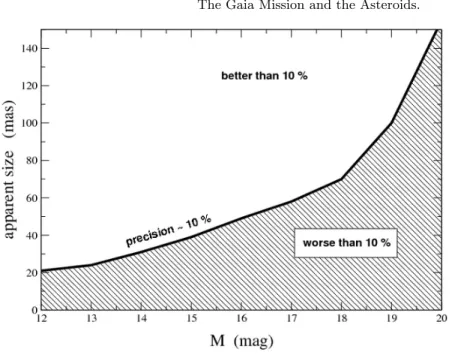
Fig. 6. The smallest size measurable with a precision of 10 % plotted as a function of the object apparent magnitude.
Since dσ is magnitude-dependent, it is possible to associate to any possible magnitude value a corresponding critical value of the size D for which the resulting relative error dD/D is equal to some given limit, like 10 %, as an example. The
result of this exercise is shown in Fig.6. In the figure, the size limit corresponding to
a relative size determination accuracy of 10 % is plotted versus the magnitude. The domain of this plot below the 10 % line corresponds to observational circumstances in which the image cannot be distinguished from that of a point-like source. At magnitude 12 it is possible to appreciate the apparent size for objects with a diam-eter of 20 mas, but at magnitude 20 this limit raises up to 150 mas. In conclusion, points below the 10 %-line in the figure correspond to observational circumstances for which the object is too far or is too faint for its angular size to be measured with an accuracy better or equal to 10 %.
5.5 Size measurement of Main Belt asteroids
In order to assess the capabilities of Gaia in measuring the sizes of Main Belt as-teroids, we take advantage of existing simulations of observations of these objects by GAia during its operational lifetime ([?]). These simulations provide the list of the transits of Main Belt objects on the field of view of the instrument, specifying the distance r from the satellite and its apparent magnitude M . Among the full set of simulated observations, we selected only those of objects for which a value of diameter d is available (taken from the most recent issue of the IRAS catalogue
range between 12 and 20. We assumed for sake of simplicity that the objects are spherical. The apparent size of the objects for each of the above observations will be obviously D = d/r. Having at disposal such a set of simulated observing circum-stances for a large sample of objects (about 2,000), it is possible to assess whether for each single detection the object’s size can be determined with a precision better (good observation) or worse (bad observation) than 10 % on the basis of the diagram
in Fig.6.
Fig. 7. Efficiency of Gaia in measuring the diameters of the Main Belt asteroids.
For any object, in general some observations will be good and others will be bad, according to the observing circumstances. Let S be the total number of observations of one single asteroid, and let s be the total number of good observations of the object, in the sense explained above. The resulting ratio ρ = s/S can be taken as an evaluation of the efficiency of Gaia in measuring the size of this asteroid.
We show in Fig. 7 the result of this exercise. Each asteroid is plotted as a
small cross in the efficiency - diameter plane. The solid line is the average value of the efficiency versus real diameter resulting from a running-box analysis. For asteroids having a size larger than 100 km the measurement efficiency is well above 50 %, and almost all observations are good. Below 20 km no good observation is
Fig. 8. Number of observations of Main Belt asteroids of different sizes, allowing a size measurement with an accuracy of 10 % or better.
possible, because the objects are either too small or too faint or both (note the group of crosses with ρ = 0 %). At the limiting size of 20 − 30 km, the measurement efficiency is only a few percent.
A slightly different plot is shown in Fig.8, where the number of good
observa-tions s is plotted against the real diameter for each asteroid. Again, the solid line is a running-box average. The crosses are rather scattered meaning that apart from the average scenario there are very different situations, depending on the individ-ual orbital and physical properties of the objects. We note that in the case of very large asteroids the observation efficiency can decrease due to the paradoxical fact that in many cases they are too bright, and they reach the CCD saturation limit
of magnitude 12 (examples are the group of crosses in Fig.8at D ' 150 km and
s ≤ 10 corresponding to the asteroids 11 Parthenope, 18 Melpomene, 20 Massalia, 39 Laetitia, 89 Julia, 349 Dembowska).
5.6 Limits and Margins of Improvement
The results discussed in the previous sections have been obtained under some simpli-fying assumptions. In particular, we assumed that the objects had spherical shapes, and that the optical properties of the emitting surfaces were homogeneous. Or, in other words, we made the assumption that the surface albedo of the objects was homogeneous throughout the surface. Moreover, even if we did not mention this
explicitly, the results shown in Figs. 5 to 8 were based on simulations in which
made. In fact, a well defined light-scattering law was assumed when running the ray-tracing part of the signal simulator. Without entering into details, the assump-tion was that of surfaces scattering the incident sunlight according to a composiassump-tion of a Lambertian and a Lommer Seeliger scattering law.
Now, we can ask ourselves whether the above simplifying assumptions are rea-sonable, and if there is some way to possibly improve the model. In this respect, the answer seems to be yes, and the way of improving the model is based on ancillary information that is expected to become available when the full set of recorded sig-nals from each object at all transits collected during the Gaia operational lifetime will be available. In particular, the idea is that of taking profit of the analysis of the disk-integrated magnitude measurements performed at each object transit. The measurement of the apparent magnitude at each transit on the Gaia focal plane is a less complicated task with respect to the determination of the astrometric position and apparent size of the object, as seen in the previous section. Given the full set of measured apparent magnitudes of an object, it will be possible to derive from that a big deal of information concerning the rotational properties (spin rate and direction of the spin axis) and overall shape, assumed for simplicity to be that of a triaxial ellipsoid. The derivation of the above parameters is described in another section of this lecture. Having at disposal the object’s pole direction and a more realistic triaxial shape, it will be possible to compute for each transit the corre-sponding observational circumstances in terms of apparent shape and orientation of the illuminated part of the body visible from Gaia at the epoch of the observa-tion. In this way, a much improved object’s model, with respect to that of a simple homogeneous sphere, will be adopted and used to derive refined estimates of the object’s size and also of the offset between the position of the barycenter and that of the photocentre during the transits for which the object becomes resolvable.
As for the choice of the scattering law, the situation is intrinsically more difficult, yet not completely hopeless. In particular, it will be possible to take profit of the fact that at least for a few objects (433 Eros, 243 Ida, 951 Gaspra, 253 Mathilde, and probably in the near future 1 Ceres and 4 Vesta) we have at disposal data taken in situ by space probes. For these objects, we have very detailed information about size, shape, spin and surface properties. The idea is then that of using this ancillary information to possibly improve the adopted scattering laws in the reduction of Gaia data. In particular, the most correct scattering law, at least for the objects of the above list, should be the one producing a better agreement between the Gaia results and the known properties of the objects.
6 The Determination of asteroid physical properties
6.1 IntroductionThe determination of asteroid physical properties will be one of the fundamental
contributions of Gaia to Planetary Science. As we have seen in $5, asteroid sizes
will be directly measured for a number of objects that should be of the order of 1, 000, according to current signal simulations. This spectacular result, however, will be only one of a longer list that includes: