Designing internal logistics processes for new manufacturing site

(1)

Designing Internal Logistics Processes for a New

Manufacturing Site

By

Dan David Cryan III

B.S. Chemical Engineering, University of Notre Dame, 2012

Submitted to the MIT Sloan School of Management and the Department of Civil and Environmental Engineering in partial fulfillment of the requirements for the degrees of

MASTER OF BUSINESS ADMINISTRATION AND

MASTER OF SCIENCE IN CIVIL AND ENVIRONMENTAL ENGINEERING IN CONJUNCTION WITH THE LEADERS FOR GLOBAL OPERATIONS

PROGRAM AT THE

MASSACHUSETTS INSTITUTE OF TECHNOLOGY JUNE 2019

The author hereby grants to MIT permission to reproduce and to distribute publicly paper and electronic copies of this thesis document in whole or in part in any medium now

known or hereafter created.

Signature of Author

Signature redacted

MIT Sloan Sch6oTof Management, Department of Civil and Environmental Engineering May 10, 2019

Certified by

Signature redacted

'f45t J. Spear, Thesis Supervisor Senior Lecturer, LT Sloan School of Management

Certified by

Signature redacted

David Simchi-Levi, Thesis Supervisor Professor of Civil and Environmental Engineering

Accepted by

Signature redacted

/Heidi

Nepf, Chair, OradiTat'e Proglam Committee Department of Civil and Environmetal Engineering

Accepted by

Signature redacted

JUN

2019

Maura Ikersin, Assistant Dean, MBA Program MIT Sloan School of Management

(2)

(3)

Designing Internal Logistics Processes for a New

Manufacturing Site

By

Dan David Cryan III

Submitted to the MIT Sloan School of Management and the Department of Civil and Environmental Engineering on May 10, 2019 in partial fulfillment of the requirements for

the degrees of

MASTER OF BUSINESS ADMINISTRATION AND

MASTER OF SCIENCE IN CIVIL AND ENVIRONMENTAL ENGINEERING

Abstract

The Boeing Company is the world's largest aerospace company and is constantly evaluating improvement opportunities to the production system. It is of ongoing interest to the company to have to tools to assess new manufacturing sites. Among the required tasks for such an effort, engineers must identify the processes and capabilities that will be needed. A critical element of this study is the system of internal logistics processes that could manage the flow of parts and material throughout a site. Planning the capacity of these processes is difficult when many of the parameters are uncertain and yet to be determined.

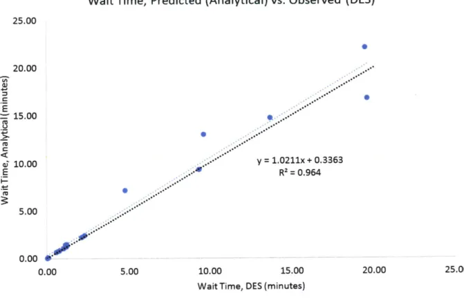
This thesis proposes a method for estimating capacity requirements of internal logistics processes by employing the concepts of queuing theory and Little's Law. Using this methodology, a process model was developed and validated by discrete event simulation to provide process planners with an understanding of the relationship and importance of numerous parameters. This understanding allows planners and management to assess the capacity requirements of the processes in terms of projected costs and performance. Values of wait times predicted by the proposed model were in strong agreement with values observed from simulation (R-squared of 96.4%; MAPE of 14.9%) suggesting that the proposed methodology represents an easy-to-use and accurate representation of process parameters. In order to improve the applicability of capacity recommendations for Boeing, further refinement is needed of underlying process parameters as well as cost modeling of threshold parameters (k and p"_max).

Thesis Supervisor: Steven J. Spear

Title: Senior Lecturer, MIT Sloan School of Management Thesis Supervisor: David Simchi-Levi

(4)

(5)

Acknowledgments

I would like to thank Boeing for hosting this internship and for their continued support of the LGO program. I owe thanks to many people, beginning with Liz Ugarph, who was

instrumental in helping me navigate the internship and grow as a student. I worked alongside an amazing team who taught me so much along the way. Thank you to everyone who was a part of this incredible experience (due to the nature of the subject matter, specific names had to be withheld).

I also owe a debt of gratitude to many other members of the LGO community at Boeing -including Nick Arch, Tom Sanderson, Andrew Byron, Jackee Mohl, Brandon Gorang, David Hahs, and Jeremy Hare - as well as my fellow LGO interns in Seattle - Mauricio Benitez, Ravi Kanapuram, Paola Molina Realpe, Jake Pellegrini, Youssef Aroub, and Skyler Stem. I'd also like to give a special thanks to our good friends at Taco Street who always provided a friendly smile and a delicious lunch at least once (or twice) a week. Thank you to my academic advisors, Steve Spear and David Simchi-Levi, for their guidance and support. Thank you to my family back in Texas who were always just a phone call away and still trekked out to Seattle to visit. Thank you to my long-time

friends spread out around the world. And finally, thank you to Sarah for her love and support throughout this whole journey.

(6)

(7)

List of Figures

Figure 1: Process Flow Diagram of Internal Logistics System ... 45

Figure 2: Number of Servers Required versus E[A]/c-t Ratio ... 51

Figure 3: Process Utilization versus E [A]/ct Ratio ... 52

Figure 4: Predicted Wait Times versus Simulated Values ... 53

Figure 5: Percent Error of Predicted Values versus E[A]/c-t Ratio ... 54

Figure 6: Predicted and Simulated Wait Times of Processes 1, 3, and 4...55

Figure 7: Fulfillment Capabilities when Managing Emergent Requests by FIFO...63

Figure 8: Fulfillment Capabilities when Prioritizing Emergent Requests ... 64

Figure 9: Recurring Cost Index of System at Baseline, 95%, and 90% Quality Levels ... 6 6 Figure 10: Predicted Queue Lengths from G/G/N Model versus Process Coefficient of V a ria tio n ... 6 8 Figure 11: Histogram of Log-normal Randomly Distributed Values of Mean = 120 a n d C O V = 1 2 5 % ... 6 9 Figure 12: MAPE of Predicted Wait Times versus E[A]/c-t Ratio of Each Process .... 70

List of Tables

Table 1: List of Assum ed Param eter Values ... 30

Table 2: Projected Utilization of Varying Number of Servers, N ... 32

Table 3: Expected Wait Times of Varying Number of Servers, N ... 33

Table 4: Expected Values of VA/NVA of Varying Number of Servers, N ... 35

Table 5: Lifecycle of an Electric Tug (per delivery)... 37

Table 6: Expected Values of VA/NVA of Varying Number of Equipment, N ... 38

Table 7: Expected Values of pn of Varying Number of Equipment, N... 39

Table 8: Expected Wait Times of Varying Number of Equipment, N ... 40

Table 9: Ratios of E[A]/c-t for Internal Logistics Processes ... 48

Table 10: Results of Capacity Planning Analysis: Servers Required... 50

Table 11: MAPE of Predicted Wait Time Values by Level of Process Variation ... 54

Table 12: Lifecycle of an Electric Tug (per delivery) with Unknown Wait Times...56

Table 13: Results of Capacity Planning Analysis of Processes 5 and 7...57

Table 14: Lifecycle of an Electric Tug for Different Levels of Process Variability...57

Table 15: Expected Wait Times of Varying Number of Electric Tugs with Low P ro ce ss V a riab ility ... 5 8 Table 16: Expected Wait Times of Varying Number of Electric Tugs with Medium P ro ce ss V a riab ility ... 5 8 Table 17: Expected Wait Times of Varying Number of Electric Tugs with High P ro ce ss V a ria b ility ... 5 8 Table 18: Lifecycle of a Daughter Cart (per delivery) with Unknown Wait Times .... 59

Table 19: Results of Capacity Planning Analysis of Processes 5, 7, and 8 ... 60

(10)

Table 21: Expected Wait Times of Varying Number of Daughter Carts with Low P ro cess V ariab ility ... 6 1 Table 22: Expected Wait Times of Varying Number of Daughter Carts with Medium

P ro cess V a riab ility ... 6 1 Table 23: Expected Wait Times of Varying Number of Daughter Carts with High

P ro cess V a riab ility ... 6 1 Table 24: Expected Fulfillment Capabilities when Managing Emergent Requests by

F IF O ... 6 2 Table 25: Expected Fulfillment Capabilities when Prioritizing Emergent Requests. 63 Table 26: Nominal Recurring Cost Factors per Number of Servers for Each Process

... ... ... ... ... ... ... . . .. ... . . 6 5 Table 27: Recurring Cost Index of Each Level of Process Variability ... 65

(11)

1 Introduction

1.1 Thesis Overview

The Boeing Company is the world's largest aerospace company and a leading manufacturer of commercial jetliners, defense, space and security systems and provider of aftermarket support services. The company is constantly undergoing continuous improvement efforts to produce the highest quality aircraft by the most effective and efficient means possible. Recently, leadership has embarked on a multi-year effort to explore improvements to its

production system design, including how to best manage the on-site logistics processes (i.e. "internal logistics") and determine the best approach to establishing new manufacturing

facilities. In order to control upfront investment costs and recurring costs of regular operations, Boeing leadership must understand how much capacity will be required to support these internal logistics processes and what impact various risk factors may have on system performance.

In order to provide a better understanding of capacity requirements and the importance of associated process parameters, this thesis will present the output of research conducted alongside Boeing leadership and operations planners. The goal of this research was to understand capacity planning in the context of the Boeing production system design, to recognize the challenges

faced by process designers, and to develop and validate a methodology to provide designers the tools needed to recommend sufficient capacity in future processes. This research effort

determined that process designers would benefit from more robust tools at their disposal to ensure that internal logistics processes are capable of meeting expected demand and variation of regular production. Previous capacity estimation efforts occasionally relied on parametric models which perversely ensured that any inefficiencies of the previous system appropriately scaled with

(12)

the new system. To counteract this problem, this thesis will recommend an analytical approach to capacity planning - based on academic research and verified by discrete event simulation - that was developed with special consideration of the demands of Boeing internal logistics processes.

In chapter one, this thesis will introduce Boeing, ongoing improvement efforts to the Boeing production system, and the specific processes known as "internal logistics." Chapter two will introduce the technical content relevant to capacity planning including queuing theory, Little's Law, and discrete event simulation. Chapter three will present how issues related to capacity planning manifest themselves in system perfonnance and the motivation for solving these issues. Chapter four will provide an overview of the analytical approach that was developed for internal logistics capacity planners using the principles of queuing theory and Little's Law. Chapter five will apply this capacity planning methodology to the anticipated system parameters to demonstrate the impact and relationship of several key variables on system performance. Chapter six will present a discussion of this analysis to provide additional

understanding around process variability, validation methods, and supporting assumptions. This thesis will conclude with chapter seven which will provide a summary of key findings and recommendations and opportunities for further study.

1.2 Problem Introduction

This thesis will attempt to solve the problems exemplified by the experience of Ashley', a Boeing engineering manager responsible for designing the logistics processes for new

manufacturing sites. Ashley leads a small team of former supply chain analysts and logistics

(13)

operators who have been assigned to the project. The following is an example of a typical work

interaction for Ashley:2

Ashley opens the email she just received from her senior manager. Estimates for the proposed warehouse are due by next Friday. He assures her that these estimates do not need to

be exact figures but does also remind her of the importance ofpresenting a design that fits within budgeted upfront and recurring costs. Ashley is not surprised by this request but still feels her blood pressure rising.

About six months ago, another engineer had worked on this problem. He took the

dimensions offive other warehouses in the manufacturing network, averaged the square footage, and rounded up a little bit to provide some "wiggle room." He had moved on to another project working on a software development effort but had left Ashley the results of his "analysis."

But now leadership wanted to understand expected design costs. Ashley had no idea if her

former colleague had scaled up his estimate for square

footage

correctly. She also had some

serious doubts about his cost numbers. She was just now starting to receive projections

from

other teams on the number ofparts that would be stored in the warehouse - but she was still

waiting on afew stragglers. Ashley thought to herself "There's no way he knew back in April how many parts would be in the warehouse... nobody can tell me that number today!"

Ashley looked back at the process flow diagram she had been working on. The first box on her slide said "Receiving."

She mused to herself "I know we need a big receiving area but how many dock doors will we need? And once those parts are off the truck, how can I possibly know how many put-away people I'll need?" She changed her attention to the next box labeled "Put-away:"

(14)

"We're going to change how we stow parts and material for this warehouse anyway.

There's nowhere in Boeing doing things this way today. How am I supposed to know how much

daily costs will be 10 years from now?"

Just then, her phone rings. ft's the supply chain analyst on her team. He wants to know if

Ashley likes the electric tug supplier he found. The electric tugs would be critical to the kit

delivery process. Ashley tells him she will take a look and call him right back.

"That's another thing," she thinks to herself "how many tugs will we need? And how

often will they go back-and-forth

from

the warehouse to the factory? "

Ashley wishes she had the answers. She's missing the data she needs and worried her

design will just keep getting squeezed by cost-conscious leadership.

Ashley's experience is not unique to Boeing - many firms could benefit from more well-defined processes for designing and evaluating systems. However, Ashley's problem is both a lack of tools and data. Not only is she unsure how to approach the problem at hand, she does not have much of the information she needs to provide a reliable recommendation.

If Ashley cannot tell her boss how much the internal logistics system will cost 10 years from now, then maybe she could tell him instead what that cost would depend on. For a system as complex as the one Ashley is designing, that recurring cost estimate depends on dozens, if not hundreds, of variables. Just picking a variable to scrutinize first may feel overwhelming.

In the absence of well-defined data (in this case, yet to be defined process parameters), this thesis will use principles of capacity planning, along with a comprehensive process model, to provide an understanding of how the system variables are interconnected. This problem statement will be expanded on in further detail in chapter three.

(15)

1.3 Internal Logistics Processes

Historically, the majority of Boeing manufacturing operations occurred in factories near Seattle, WA. Manufacturing operations included the fabrication of (mostly aluminum)

components, assembly of sub-assemblies, final assembly, paint, and systems tests. Over time, Boeing expanded its supply base across the United States and international geographies. To manage the complexity of an international supply chain, Boeing has made significant investments in its logistics capabilities.

Within Boeing, there is a supply chain division that manages a significant variety of logistics activities including material ordering, transportation, on-site receiving, storage of material, and conveyance of material from warehouses to production workers on the factory floor. External logistics encompasses all movement and management of material while that

material is not located on a Boeing site. This includes material ordering, transportation, the estimation and tracking of shipping rates, among other activities. Therefore, internal logistics includes all logistics activities that occur while material is located on a Boeing site. Internal

logistics includes a wide variety of processes that fall under the umbrella of processes traditionally known as "materials management." Internal logistics within the context of this thesis will be divided into nine sub-processes:

1. Receiving 2. Quality Check 3. Put-away

4. Pick, Kit, and Integrate 5. Kit Staging

(16)

7. Tug Unloading

8. Consumed Kit Processing 9. Shipping

Additional process details of the internal logistics system will be provided in chapter five.

1.4 Process Improvement Efforts and Capacity Planning

In order to ensure that Boeing is competitive in current and future t markets, leadership is regularly managing studies to identify and implement improvements to the production system. Following broader trends in the aerospace industry, Boeing has pushed for increased design-for-manufacturing and model-based systems engineering. Ongoing efforts include creating the tools and processes necessary to define the production system needs of a "greenfield" manufacturing environment. Ashley's team - focused on the internal logistics processes - is one of many teams working on this project.

At the core of Ashley's problem is the question of process capacity. To determine the number of truck unloading bays in the receiving area or the number of semi-automated put-away stations required, she will need to understand the capacity of these processes. She will also need some criteria at her disposal for selecting the right amount of capacity to recommend. How much capacity will be enough? Is it better to have too much capacity than not enough? Which variables should be optimized and which are inconsequential to her design?

(17)

2 Technical Content Review

This section will provide an overview of the technical content underlying the capacity planning methodology developed over the course of this thesis project. The concepts introduced

in this chapter - queuing theory, Little's Law, and discrete event simulation (DES) - will be combined into a detailed methodology for identifying capacity requirements within the context of Ashley's internal logistics planning effort.

2.1 Queuing Theory

Queuing theory relates to the study of systems by which requests (or customers, or products) arrive to a system and are serviced according to some pre-determined discipline. Congestion occurs when there are more service requests than available servers which causes a queue to develop. Queuing theory is a well-established subject with applications across a variety of fields, including call service centers, supermarket checkout lines, gas stations, and IT systems. A. K. Erlang is widely regarded as one of the original founders of queuing theory for his work studying telephone exchange systems in the early 1900s [1].

The M/M/c queue, or Erlang-C model, is a commonly used multi-server queuing model relevant for systems with more than one server. Arrivals of service requests are probabilistic with inter-arrival times following a Poisson distribution. The processing time of each server is assumed to be exponentially distributed and independent of other servers. This model assumes no maximum queue length, allowing for infinite queue size. It also assumes no queue

abandonment will occur (such as an impatient customer service caller hanging up while still on hold) [2].

The Erlang-C model is defined by:

(18)

Where: n

n = number of servers

A *

x=-o /I= arrival rate

o y = service rate

0 B(n, x) =(xn/n!)/(1 +X + /2! + /3! +..- + xn/n!)

o This is the Erlang-B function which accounts for the probability of service requests arriving to a system with no available servers.

The average queue length, Lq, is given by the following equation [3]:

L = x C(n, x) (2)

q n-x

An approximation of this model is useful for simplifying this equation for systems of known standard deviations of inter-arrival and service times [4]:

2 (n+1) C2+C2 L '= x ccS(3) q 1-p 2 Where: Sp= capacity utilization = -n/i

* CA = _{coefficient of variation, interarrival}_times

* Cs = _{coefficient of variation, service times}

This simplified model is known as the G/G/N model. Like the Erlang-C model, it may only be used for stable systems where p<l, otherwise the queue length would continue to grow to infinity as additional requests arrive [3], [4].

The models presented thus far all assume that service requests are processed according to the principle offirst-in/first-out (FIFO). That is, all requests are prioritized equally and are serviced

(19)

in the order in which they arrive. However, in certain situations it may be desirable for system managers to prioritize some requests over others.

Non-preemptive prioriry queues describe systems under the following conditions:

" Processing of the request(s) currently being served is completed even if requests of higher priority arrive;

" Each priority class has a separate queue;

* When a server becomes free, the request from the head of the highest priority queue is processed by the available server [5].

For non-preemptive priority queues, Kleinrock's conservation theorem is applicable [5]

>k=1 PkWk -X R (4)

1-p

Where:

" K = _{number of priority classes, k}= 1, ... , K " Wk = mean wait time of classk service requests

0 R = mean residual service time upon arrival

This theorem provides operations managers with two powerful conclusions that guide their understanding of the behavior of systems of non-preemptive priority queues:

" The weighted average of wait times is constant no matter the queuing discipline employed.

" Any attempt to modify the queuing discipline so as to reduce some value of Wk will force an increase in the value of some other Wk [5].

This concept will prove useful when analyzing whether or not to prioritize emergent (non-scheduled) kit requests.

(20)

2.2 Little's Law

Little's Law states that the long-term average number, L, of customers (or products, or service requests...) in a system is equal to the long-term average arrival rate, A, multiplied by the average time, W, a customer spends in the system. Simply put:

L=AxW (5)

This theorem holds true for stable systems, which excludes situations such as startup or shutdown. It was first published in 1954 [6]. In 1961, Little published a proof of Little's Law, showing no such situation existed in which it did not hold true [7].

This theorem is useful for studying queuing systems because it relates expected queue lengths to expected wait times in an intuitive manner: the average number of "customers" in the queue divided by the rate of arrival will be used to calculate expected queue wait times.

2.3 Discrete Event Simulation and Monte Carlo

Discrete event simulation (DES) is a widely used operations management technique for assessing the performance of a physical system in a virtual setting. System events are modeled according to discrete time intervals. Random number generation is used to model probabilistic behavior related to random variables (such as arrival and service rates). DES can be useful for diagnosing a variety of process issues and can be tied to any number of performance indicators such as worker utilization, on-time delivery rate, scrap rate, etc.

In the context of analyzing queue behavior, a simple DES model can simulate service requests entering a queue, waiting for an available server, undergoing processing, and exiting the system. Such an analysis will be useful for testing the validity of analytical models presented in previous sections. Additionally, DES can provide an estimate of maximum queue length which is not easily obtained from available analytical models [8].

(21)

Running consecutive DES models produces a data set of estimated performance indicators, 0, similar to established Monte Carlo analytical techniques. For N consecutively executed model runs, the standard error (SE) of 0 is the standard deviation of the sampling distribution from N samples [9].

(22)

3 Capacity Planning Problem

In chapter one of this thesis, an introduction was provided covering the ongoing

improvement efforts focused on assessing and redesigning internal logistics processes supporting the production system. Chapter three will expand on the ongoing process improvement efforts by providing a more thorough understanding of the issues affecting internal logistics process

performance and why capacity planning was selected as the central problem under consideration for this thesis.

3.1 Factors Affecting System Performance

Leadership has an extensive selection of metrics at their disposal for measuring the

performance of internal logistics processes. In general, managers will concern themselves with the effectiveness and efficiency of their operations. Considering the effectiveness and efficiency of Boeing internal logistics processes, this thesis proposes that leadership pay close attention to the following three factors: time-in-system, variability, and cost.

3.1.1 Time-in-System

The total time that parts and material spend in the production system has a significant impact on operating expenses. By the principles of Little's Law (introduced in the previous chapter), the longer that parts and material remain in the factory on average, the more parts and material there will be in the factory at any given time. Therefore, slow inventory turnover can lead to numerous other issues impacting system effectiveness and efficiency:

Floor Space

Excessive raw material and work in process (WIP) inventory leads to the need for additional floor space throughout the production system. Acquiring additional floor space in a

(23)

manufacturing context can add significant operating and capital expenses. When operating areas are no longer able to support necessary inventory levels, firms must invest in additional storage facilities, which can be either temporary (i.e. renting warehouse space from a third party) or permanent (i.e. capital expenditures on facility expansion).

Materials Management

Managing excessive inventory places additional strain on limited materials management resources, including warehouse staff and inventory control processes.

Capital Opportunity Costs

Excessive material inventories tie up a firm's working capital. This can lead to limited investment in necessary capital expense projects or other more attractive investment

opportunities. Poor Quality

In many cases, excessive inventory can lead to challenges with maintaining product quality. With more parts on the floor, it's more difficult for firms to ensure the quality of every part as it makes its way through production. With more time spent in system, parts are exposed to the risk of product damage for longer time intervals. Poor quality means higher raw materials costs, higher labor costs, and possibly missed sales or damage to reputation.

3.1.2 Variability

In an operations setting, variability can manifest itself in any number of ways. In the context of queuing theory, as detailed in chapter two, variability in arrival and service times translates into increased average queue sizes. Increased queue sizes directly relates to increased time-in-system. In highly variable systems, firms may be forced to invest in extra capacity to avoid excessive non-value-added time of parts and material waiting in queues.

(24)

Variability can also be understood in terms of process quality. A tightly controlled "six sigma" process will produce few defects and require little rework. By contrast, a poorly controlled process will produce excessive defects, leading to increased raw material costs, decreased labor and equipment efficiency, and increased demands on system capacity. It is

imperative that operations managers understand the relevant sources of variability, the impact on system performance, and how they can manage and limit variability within the system design.

3.1.3 Cost

In general, both time-in-system and variability contribute to the cost of operating the internal logistics system. While cost efficiency may be a shared goal across firms, the extent to which firms dedicate their time and resources to cost avoidance certainly varies. In designing

logistics processes, costs associated with the system should be categorized by what is either recurring or nonrecurring.

Nonrecurring Costs

All one-time costs associated with setting up the system are nonrecurring costs. These include capital expenses associated with purchasing (or refurbishing) equipment and facilities. Recurring Costs

All regular operating expenses associated with running the system can be thought of as recurring costs. This includes labor, overhead such as electricity, raw materials, and

facility/equipment maintenance.

3.2 Process Design

At this point it is useful to return to the questions plaguing Ashley, the process engineer introduced in chapter one:

(25)

How much capacity should be acquired to support internal logistics processes at a new

manufacturing site? Which processes should be transferred

from

existing operations and which

processes require improvements? How much space will be required to support these processes? How much will it cost to implement these processes in a new manufacturing space?

A common thread underlying these questions is the concept of capacity. When process capacity is significantly in excess of demand, the firm's cost efficiency is negatively impacted. Resources allocated to acquiring the excessive capacity are unproductive. When capacity is too low, the firm's effectiveness and efficiency are both negatively affected. Customer service could be impacted resulting in brand damage and missed sales. Striking the right balance between too much and not enough capacity allows firms to meet customer demand in an efficient manner.

For these reasons, this thesis will focus on capacity planning in the context of Boeing's on-going internal logistics improvement efforts. Specifically, how much capacity should be acquired to support internal logistics operations at a new manufacturing site? The answer to this question will depend on many of the factors already mentioned. What do these new processes look like?

How well will they perform? How will performance variability, such as the amount of rework required, affect capacity demands?

To answer these questions, a methodology for identifying the number of servers needed at each process step will be proposed based on principles of queuing theory and Little's Law. A similar methodology will be developed for identifying the amount of equipment needed to support operations. Additionally, a number of assumptions will be presented around system parameters and operating discipline, especially related to the handling of emergent requests otherwise known as "rework."

(26)

An understanding of the current state of internal logistics processes and areas of improvement will be developed. Then the proposed methodology will be applied to the envisioned processes to determine how much capacity is required and the behavior of various factors' effect on this determination.

(27)

4 Methodology Overview

This chapter will explain the methodology that will be used to determine capacity

requirements of proposed internal logistics operations for a manufacturing site currently under assessment. First, the supporting assumptions need to be established around key parameters of these proposed processes. Second, an approach for determining the number of servers needed for each process will be presented. Following that, another approach for determining the number of pieces of equipment needed will be presented. Chapter four will conclude with a third approach for calculating expected wait times of emergent part requests, which can be understood as non-standard operations, and the effect prioritization of certain requests may have on non-standard operations.

4.1 Process Assumptions

In planning the design of a future production system, the exact numerical values of certain process parameters are mostly unknown. This analysis will address this issue by making

reasonable assumptions of parameter values based on discussions with operations leadership and from observation of existing processes. A sensitivity analysis will be provided for certain

selections of these parameters. Additionally, modeling efforts will anticipate the needs of

planners who will gain access to more mature parameter estimates over time, so the manipulation of these values in the model will be relatively user-friendly.

Other exact values relevant to ongoing Boeing planning conversations were obfuscated for the sake of confidentiality. The remainder of this section will present the significance of each process parameter and will then provide the assumed value used for capacity planning analysis, where appropriate.

(28)

Production Rate

Production rate refers to the number of shipsets (ss) to be produced per month. One shipset is the equivalent of one commercial jetliner. For capacity planning purposes, it is helpful to design operations to support production at 100% of projected rate. Therefore, values used in this analysis for production rate range from 10 to 15 ss/month.

While an understanding of capacity requirements at rates less than 100% of full

production will be useful for planners concerned with initial start-up stages of operation, partial rate analysis and/or rate ramp-up analysis were excluded from the scope of this thesis.

Parts per Shipset

Parts per shipset is equal to the number of individual parts that will be processed by internal logistics for each shipset. A bill of materials (BoM) for an aircraft may include hundreds of thousands of parts [10]. For this context, "parts" also include materials that will not be

installed on a shipset (such as hand tools), because these materials will still be needed by

manufacturing personnel to complete their required work. The parts per shipset value will consist of all parts and materials that a production worker needs to do their work, including supplier-provided "hard parts," fasteners, consumables, tools, and hazardous material. This analysis assumes a value of 100,000 parts/ss.

Number of Point-of-Use Locations

Point-of-use (POU) locations are the areas within the factory where integrated kits (i-kits) are delivered by logistics personnel to be consumed by production workers. I-kits contain all the parts that a production worker needs to complete their scheduled "job" including all "hard parts,"

fasteners, consumables, tools, and hazardous material. Production workers may complete one to fourjobs (or more) per shift. Production workers at POU locations can be thought of as the

(29)

"customers" of the internal logistics system. As the number of POU locations increases within the system, the complexity of operations for internal logistics processes also increases. For the proposed production system under consideration the number of POU locations was assumed to be equal to 140.

Integrated Kit (i-kit) Delivery Demand

I-kit delivery demand is related to the number of total i-kits that must be delivered to all POU locations over a set period of time (usually per shift). In order to estimate this parameter, assumptions were made regarding the frequency of delivery to each POU location. The delivery frequency is dependent on the lengths of jobs to be completed at that POU location, where one i-kit corresponds to one job. Based on these factors, baseline demand for i-kits was determined to be ~422 i-kits/shift.

Baseline demand is different from total demand in that baseline demand ignores the

emergent kit deliveries that will be requested periodically throughout a shift to account for

missing parts, incomplete kits, product damage, or operator mistakes. Logistics planners anticipate that a certain number of emergent kits (e-kits) will need to be prepared and delivered on an ad hoc basis by internal logistics processes to support less-than-perfect system quality. Delivery On-time-in-full (OTIF) Percentage

The first parameter addressing system quality is the percent of deliveries made on-time and in-full (OTIF%). If a delivery arrives late (or not at all) or is missing some number of parts, planners assumed a process will be in place for production workers to request a replacement delivery. These e-kit requests are assumed to be solely caused by quality issues associated with processes upstream from production operations (i.e. internal logistics). Baseline OTIF% was assumed to be equal to 99.5% or approximately five quality defects per 1,000 deliveries.

(30)

Production Quality Percentage

The second parameter addressing system quality is the production quality percentage (PQ%). This parameter is related to the number of e-kits that must be delivered due to issues stemming from manufacturing operations, such as product damage. Baseline PQ% was assumed to be equal to 99.0% or approximately 10 quality defects per 1,000 production jobs.

Truck Arrivals per Shift

A number of other more granular assumptions were also made in relation to each individual process within the internal logistics system. One example of these more granular assumptions is the average number of truck arrivals to receiving per shift. This value was assumed to be approximately 30 trucks/shift. For calculating the number of servers needed for unloading trucks, this assumption guides planners' understanding of how many trucks must be unloaded during each shift.

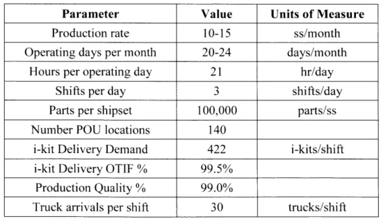
A complete list of assumed parameter values is compiled in Table 1.

Table 1: List of Assumed Parameter Values

Parameter Value Units of Measure

Production rate 10-15 ss/month

Operating days per month 20-24 days/month

Hours per operating day 21 hr/day

Shifts per day 3 shifts/day

Parts per shipset 100,000 parts/ss

Number POU locations 140

i-kit Delivery Demand 422 i-kits/shift

i-kit Delivery OTIF %

99.5%

Production Quality % 99.0%

(31)

4.2 Capacity Planning: Servers

To make a determination of the number of servers required to support a process, this analysis will use the principles detailed in chapter two related to queuing theory and Little's Law. First, assumptions related to process parameters will be clearly defined. Second, a

sensitivity of expected utilization and queue length will be analyzed with respect to the number of process servers. Finally, the expected wait time will be calculated and normalized with respect to the process cycle time. These ratios will be useful because they are directly related to the non-value-added time experienced by inventory during manufacturing. As detailed in chapter three, efforts to control and reduce time-in-system provides numerous benefits related to the

effectiveness and the efficiency of the manufacturing process.

To illustrate this methodology, an example will be provided for the truck receiving process which represents the first process of the internal logistics system.

As already mentioned, the average truck arrival rate is estimated to be 30 trucks/shift. A = 30 trucks/shift

A = 0.07 trucks/min

The coefficient of variation of truck arrivals needs to be assumed (the exact value is unknown, but could be estimated more precisely by conducting time studies of current receiving operations). For this example, this value was assumed to be 100%.

CA = 100%

Next, the average and coefficient of variation for truck unloading cycle times must also be assumed. The following values were determined to be reasonable starting points:

Cycle time, unloading = 120 min/truck 1

(32)

Cs = 50%

A reasonable range of n values is now necessary to conduct a sensitivity analysis. After some brief trial and error, a range from 7 to 13 is found as reasonable.

n = {7,8,9, ... ,13}

For each value of n, the time available is determined by the shift length of that process. All shifts are assumed to be 7 hours in length (21 operating hours per day / 3 shifts per day).

Available time (min/shift) = {2940,3360,3780,..., 5460}

The maximum service rate is then also calculated for each value of n. Available time

Maxmum service rate (trucks/shif t) = = 24.5, 28.0, 31.5, ... , 45.5}

The expected utilization is then calculated for each value of n. E [ A]

pE[A = {1.224, 1.071, 0.952, ..., 0.659}

Maximum service rate

Note that this calculation matches the equation for capacity utilization presented in chapter two: 'k ny (0.07 trucks/min) (7 = = 1.224 (7 x 0.0083 trucks/mmn)

Table 2 displays the results of the sensitivity analysis thus far:

Table 2: Projected Utilization of Varying Number of Servers, N

n Available time Maximum service rate p

(min/shift) (trucks/shift) 7 2940 24.5 122.4% 8 3360 28.0 107.1% 9 3780 31.5 95.2% 10 4200 35.0 85.7% 11 4620 38.5 77.9% 12 5040 42.0 71.4% 13 5460 45.5 65.9%

(33)

The G/G/N queuing model can now be applied to calculate the average number of trucks waiting in queue for each value of n, so long as the value of pn < 100%.

pn= (n-+- )2 + Cs2

Ln=9 =-x C == 10.6 trucks

1 - pn=9 2

Little's Law can then be applied to determine the expected time each truck spends in queue, on average, for each value of n.

L= AxW

Ln=9 10.6 trucks 7 hours 60 min

W ' x x = 147.7 min

A 30 trucks/shift 1 shift 1 hour

Table 3 displays the updated sensitivity analysis complete with expected wait times.

Table 3: Expected Wait Times of Varying Number of Servers, N

n p Lq W (minutes) 7 122.4% -8 107.1% -9 95.2% 10.6 147.7 10 85.7% 2.1 29.7 11 77.9% 0.8 11.7 12 71.4% 0.4 5.5 13 65.9% 0.2 2.8

From the perspective of a designer wishing to select a value of n, there are two competing forces related to the system efficiency that must be balanced:

* Utilization, p. The utilization of the system is tied to the process efficiency. Utilization at

100% means that the system is meeting demand with the minimum required resources.

Utilization less than 100% means that there is additional unused capacity within the system. In general, utilization should be maximized, with some additional capacity reserved to handle typical process variability.

(34)

* Queue wait time, W. The time-in-system, another measure of process efficiency, is directly related to the time material waits to be processed. As wait times increase, additional costs are incurred related to working capital costs, facilities cost, materials management expenses, and potential quality issues. In general, wait times should be minimized.

This thesis proposes that system designers relate these competing variables by using the following ratio:

VA _ Cycle time

NVA Wait time

Where:

" VA = Value-added time or the productive processing time

" NVA = Non-value-added time or the non-productive time material spends in the system

Value-added time in this context can be defined as the productive time or the processing time

that directly adds value to the customer. Value-added time is estimated by the cycle time of the process, which is a significant simplifying assumption. Non-value-added time is all non-productive time and can be estimated by the wait times experienced within the process. As needed, non-value-added time will also be estimated by subtracting value-added time from all available time. Using these simplified definitions and the ratio in Equation 7 allows the process designer to select the value of n that satisfies the following objective function:

VA

maxpV _NVA > k (8)

This objective function provides the designer with a heuristic approach to select a reasonable value for n. Table 4 shows the updated sensitivity analysis with calculated values of VA/NVA.

(35)

Table 4: Expected Values of VA/NVA of Varying Number of Servers, N n p Lq W (minutes) VA/NVA 7 122.4% - - -8 107.1% - - -9 95.2% 10.6 147.7 0.8 10 85.7% 2.1 29.7 4.0 11 77.9% 0.8 11.7 10.3 12 71.4% 0.4 5.5 21.8 13 65.9% 0.2 2.8 42.3

According to the proposed design rule, for k = 3,3 the designer would select n =10.

This value of n corresponds to the maximum rate of utilization for which VA/NVA > k. For the

example provided, this means that 10 truck bays should be built to unload trucks in a receiving area matching these process parameters.

4.3 Capacity Planning: Equipment

It will also be incumbent on system designers to use these principles for similarly selecting the amount of equipment needed to support internal logistics processes. A good example of how this methodology can be applied is the case of selecting the number of electric tugs to be

deployed in the system. These electric tugs will be manually operated and used for moving material to and from the production floor.

First the demand for tugs must be determined. This demand will be equal to the rate of tug deliveries that must be completed to support full production. Deliveries of material can be categorized by one of two types of deliveries: standard or emergent.

* Standard deliveries will be made according to a daily schedule that pulls from a ready-to-be-used buffer of i-kits (in the kit staging area) to deliver material "just-in-time" to the

3 A VA/NVA ratio of 3:1 is considered "world-class" by industry experts. However, the metric of VA/NVA used in this thesis assumes that all process cycle time is value-added, which is almost certainly

not the case. Therefore, considerable tuning would be worthwhile to identify the right value of k. Tuning this heuristic did not fall within the scope of this project, but would make for an interesting opportunity for additional study. This topic will be discussed in further detail in chapters six and seven.

(36)

production floor. Because tugs can deliver more than one i-kit per departure, the average number of i-kits that will be delivered for each trip should be equal to the maximum tugging capacity of each tug. A reasonable starting assumption is that each tug will be able to deliver four i-kits per delivery. If assumed i-kit delivery demand = 422 i-kits/shift, then the expected number of standard deliveries will be 106 deliveries/shift.

0 Emergent deliveries will be made as demand for emergent kits arises throughout

standard operations. Emergent demand could be due to improperly prepared i-kits, miss-delivered i-kits, or production quality issues. Using assumed values of delivery OTIF%=

99.5% and PQ% = 99.0%, the expected number of emergent deliveries will be six

deliveries/shift.

Therefore, the total rate of tug deliveries will be expected to be 112 deliveries/shift. Next, the estimated time-in-system (per delivery) must be calculated. This time will be heavily dependent on assumed values for cycle times of each process step as well as expected tug downtime due to equipment failures or regular battery recharging. Additionally, at certain high-traffic steps throughout the delivery process, the tug may be waiting in queue to be loaded or unloaded. These wait times were also calculated using G/G/N and Little's Law as described in the previous section. Table 5 details the assumptions of the underlying values needed to calculate tug time-in-system (per delivery):

(37)

Table 5: Lifecycle of an Electric Tug (per delivery)

Description Time VA or NVA Explanation (min/delivery)

Cycle time, tug loading 5.0 VA Time to load tug at warehouse staging area

Cycle time, tug convey 12.0 VA Time for tug to drive from (from warehouse to factory) warehouse to each POU delivery

location

Cycle time, receipt at POU 5.0 VA Total time for tug to deliver i-kits

to each POU location

Cycle time, tug convey 12.0 VA Time for tug to drive back to

(from factory to warehouse) warehouse from factory

Cycle time, tug unloading 10.0 VA Time to unload tug at kit return

area

Total VA time-in-system 44.0 min/delivery

Waiting, tug loading 5.6 NVA Wait time for tug to be loaded at

warehouse staging area

Waiting, tug unloading 1.9 NVA Wait time for tug to be unloaded

at kit return area

Downtime, average per 0.4 NVA Average tug downtime, assuming

delivery 2 hours downtime per day

Total NVA time-in-system 7.9 min/delivery_ Total time-in-system 51.9 min/delivery

Next, Little's Law can be used to determine the

delivery demand at 100% capacity utilization.

number of tugs, L, required to meet this

A = 112 deliveries/shift = 16.0 deliveries/hr W = 51.9 mi/delivery = 0.87 hr/delivery L=2LxW / deliveries h r\ L =16.0 deieis X 0.87- =r 13.8 hr delivery)

This approach suggests that 13.8 tugs, on average, will be needed to satisfy expected

delivery demand at 100% utilization.

Similar to the previous analysis for server capacity, a sensitivity analysis can now be used to

calculate expected utilization for increasing values of n, the number of tugs to be acquired for

(38)

n = {14, 15, 16, ... , 19} The capacity utilization calculation is straightforward:

=1=oo% 13.8

Pn=14 - 13.8 = 98.8%

n 14

The VA/NVA ratio can also be calculated. First, value-added time is related to the rate of

tug-deliveries and the total VA time per delivery. A modified version of Little's Law can be used:

S deliveries min

VAn=14 = A x WVA = 16.0 x 44.0 = 704 min/hr

hr _delivery

This equation suggests that value-added time is constant with respect to n. Upon further reflection, this appears to be reasonable. The total value-added time experienced by the deployed tugs in the system should not change depending on the number of tugs. Value-added time, in this case, is a function of the work that must be completed and the percentage of time workers spend performing that work out of all available worker time.

Therefore, non-value-added time with respect to n should be determined by first calculating

the total amount of available time as a function of n and then subtracting value-added time.

NVAn=14 = (Available time),=₁₄ -VAn=14

min min

NVAn=14 =14 * 60 - 704 =136 min/hr

hr ) hr

From this equation, it is clear that non-value-added time will increase with the value of n. Table 6 shows the sensitivity analysis for the range of n values with VA/NVA ratios calculated:

Table 6: Expected Values of VA/NVA of Varying Number of Equipment, N

n p VA (m NVA( m VA/NVA hr hr 14 98.8% 704 136 5.1 15 92.2% 704 196 3.6 16 86.4% 704 256 2.7 17 81.3% 704 317 2.2 18 76.8% 704 377 1.9 19 72.8% 704 437 1.6

(39)

Observation of these results yields an interesting discovery. Unlike the previous method for analyzing servers, the value of VA/NVA decreases with respect to the amount of equipment in use (tugs deployed, in this example). This leaves a system designer with two options:

" Select the value of n which maximizes both utilization and VA/NVA (in this case, n = 14); * Or, determine another efficiency metric that can be used to provide sufficient capacity

buffer.

This methodology proposes that the probability of no available equipment is a worthwhile

efficiency metric to examine further. If a binomial distribution is applied to the condition of equipment availability (equipment is either available or it is not available), then the probability of no available equipment can be calculated by the following simple relationship:

P(no equip. available) = pf (9)

This metric is added to the sensitivity analysis shown in Table 7.

Table 7: Expected Values of p of Varying Number of Equipment, N

min min

n p VA( ) NVA( ) VA/NVA pn

hr hr 14 98.8% 704 136 5.1 84.2% 15 92.2% 704 196 3.6 29.6% 16 86.4% 704 256 2.7 9.7% 17 81.3% 704 317 2.2 3.0% 18 76.8% 704 377 1.9 0.9% 19 72.8% 704 437 1.6 0.2%

What this methodology is now in need of is an understanding of what is a good value of pn. The probability of no available equipment is only a useful metric in that it tells the designer the likelihood of a worker in the system waiting for a piece of equipment to become available at any given time. Framed this way, a probability of 80-100% seems unacceptably high, due to the

(40)

This analysis can be progressed by making an assumption regarding expected wait time. If a worker in the system finds that no equipment is available, then the next piece of equipment to come available must be in the process of finishing its delivery cycle, up to that point in the cycle. A uniform distribution can be applied to the random chance a worker finds herself waiting for a piece of equipment to come available. It is as equally likely that the delivery cycle just started, as it is to being a split-second from completion, as it is to being somewhere in the middle.

Therefore, given that no equipment is available, the expected wait time for the next available piece of equipment can be calculated by dividing the average process cycle time by two:

1 total cycle time

E [wait time for next available equip., given no avail. equip.] = - x ( 10)

2 (10

From this value, the expected average wait time for any worker in the system is equal to the

probability of no available equipment multiplied by the expected wait time when no equipment is available.

E [wait time for next available equip.] = ₂ x total cycle time

ni

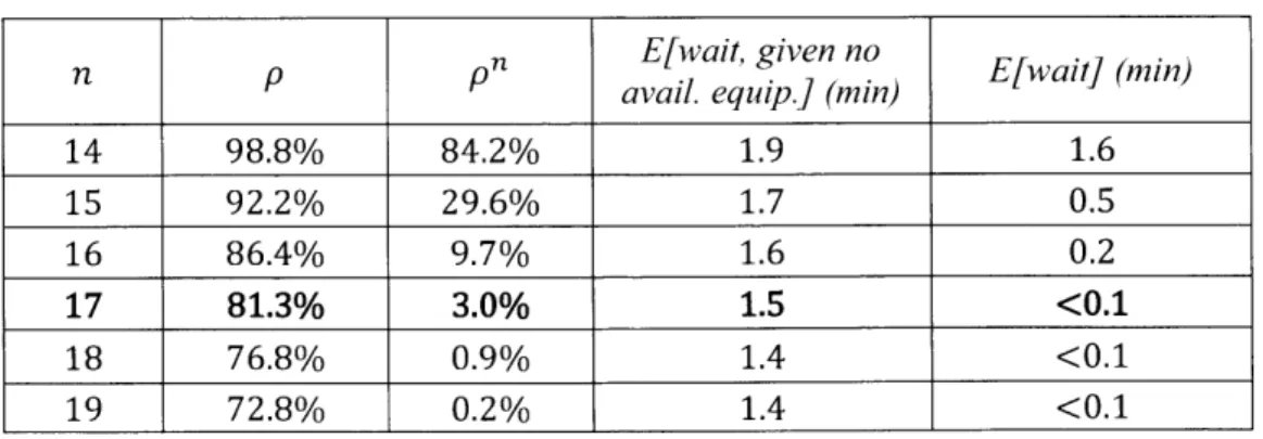
These metrics are also added to the sensitivity analysis (with VA, NVA, and VA/NVA removed) as shown in Table 8.

Table 8: Expected Wait Times of Varying Number of Equipment, N

n p pu n E[wait, given no E[wait] (min)

avail. equip.] (min)

14 98.8% 84.2% 1.9 1.6 15 92.2% 29.6% 1.7 0.5 16 86.4% 9.7% 1.6 0.2 17 81.3% 3.0% 1.5 <0.1 18 76.8% 0.9% 1.4 <0.1 19 72.8% 0.2% 1.4 <0.1

(41)

It is reasonable to assume that factory workers (as well as management) would want the expected wait time for equipment to be roughly zero. Setting the constraint that pf < 5% provides expected equipment wait times roughly equal to zero (E[wait] < 6 seconds). This suggests the system designer should select n = 17 because this is the value of n for which utilization is maximized and pf 5%.4

4.4 Calculating Expected Wait Times of Emergent Requests

As previously discussed, the impact of managing emergent kit requests must also be considered. The scope of this analysis will include two different management methods for processing emergent kit requests alongside standard operations: (1) First-in/first-out (FIFO) and (2) Emergent Request Prioritization.

4.4.1 Method 1: First-in/first-out (FIFO)

Kit requests will be processed on a first-come, first-serve basis. This approach minimizes the impact that emergent kit requests have on standard i-kit preparation, staging, and delivery. For example, say there is one i-kit in the queue and one i-kit being processed in the kit staging area, at any given time, on average. If an emergent kit request arrives to the queue, the worker(s) in that area would process the i-kit already in the queue before beginning to process the emergent kit request.

Because e-kits are processed with the same priority as standard i-kits, calculating the expected wait time for e-kits under this approach is identical to calculating the expected wait

4 Note that p" max is similar to the design variable of k introduced in the previous section. The relationship between these design variables - and how the selection of threshold values impact design outcomes - will be discussed in further detail in chapters six and seven.

(42)

time of any standard i-kit. Therefore, the expected e-kit wait time is equal to the average wait time of all i-kits through that process:

E(e-kit wait time] = E[i-kit wait time] = WV7 (12)

4.4.2 Method 2: Emergent Request Prioritization

The reasonable alternative approach is to prioritize emergent kit requests as soon as they arrive. Workers will finish whatever is already in process, then begin working on the emergent request before working on any other i-kits already in the queue. This approach provides the benefit of minimizing the amount of wait time experienced by e-kits, but should also introduce a corresponding increase in the average wait time experienced by standard (regularly scheduled) i-kits.

This management approach can be modeled as a non-preferentialpriority queue (as introduced in chapter two). Calculating the expected wait times of e-kits requires the system designer to understand the expected wait time of only the first item in the queue. There is some probability that an e-kit arrives to find an empty queue and at least one available server. In this case it will immediately begin to be processed by an available server. The probability that all servers are occupied (busy) when arriving to the process area is equal to pl.5

P(no servers available) = pf

If no e-kits are already waiting in the queue, the e-kit arriving to find no servers available will immediately go the front of the queue. Given that no servers are available, the expected wait time of the first request in the queue can be modeled as the average cycle time of the process

5 _{This concept is equivalent to equation 9 introduced in the previous section regarding equipment capacity}