On concentration inequalities for equilibrium states in lattice and symbolic dynamical systems

(1)

HAL Id: tel-03152537

https://tel.archives-ouvertes.fr/tel-03152537

Submitted on 25 Feb 2021

HAL is a multi-disciplinary open access archive for the deposit and dissemination of sci-entific research documents, whether they are pub-lished or not. The documents may come from teaching and research institutions in France or abroad, or from public or private research centers.

L’archive ouverte pluridisciplinaire HAL, est destinée au dépôt et à la diffusion de documents scientifiques de niveau recherche, publiés ou non, émanant des établissements d’enseignement et de recherche français ou étrangers, des laboratoires publics ou privés.

On concentration inequalities for equilibrium states in

lattice and symbolic dynamical systems

Jordan Moles

To cite this version:

Jordan Moles. On concentration inequalities for equilibrium states in lattice and symbolic dynamical systems. Mathematical Physics [math-ph]. Institut Polytechnique de Paris; Universidad Autónoma de San Luis Potosí, 2020. English. �NNT : 2020IPPAX102�. �tel-03152537�

(2)

626

NNT

:

2020IPP

AX102

On concentration inequalities for

equilibrium states in lattice and symbolic

dynamical systems

Th èse de doctorat de l’Institut Polytechnique de Paris pr épar ée à Ecole polytechnique and Universidad autonoma de San Luis Potosi ´

Ecole doctorale n 626 Ecole Doctorale de l’Institut Polytechnique de Paris (IPParis)

Sp ´ecialit ´e de doctorat : Physique

Th èse pr ésent ée et soutenue à Palaiseau, le 18 d écembre 2020, par

J

ORDAN

M

OLES

Composition du Jury :

Frank Redig

Professeur, Universit ´e de Delft, Pays-Bas Pr ´esident Sandro Vaienti

Professeur des universit ´es, Aix-Marseille Universit ´e Rapporteur Aernout van Enter

Professeur ém érite, Universit é de Groningen, Pays-Bas Rapporteur Sandro Gallo,

Professeur assistant, Universit é de Sao Carlos, Br ésil Examinateur Jean-Ren é Chazottes

Directeur de recherche, Ecole Polytechnique Co-directeur de th `ese Edgardo Ugalde

(3)

(4)

Acknowledgements

First of all, I would like to express my deepest gratitude to my research super-visors Jean-Ren ´e Chazottes from Ecole Polytechnique and Edgardo Ugalde from the Universidad Autonoma de San Luis Potosi who co-directed this the-sis with patience and willingness. It was a great privilege to do research under their expertise and guidance.

I would like to pay my special regards to the president of the jury and professor Frank Redig for the enlightening collaboration and his great advice about the two dimensional Ising model.

I am indebted to professor Aernout van Enter for invaluable discussions which helped to refine this work and for accepting to be rapporteur.

I thank professors Sandro Vaienti and Sandro Gallo for accepting respec-tively to be rapporteur and member of the jury and for their helpful comments and suggestions to improve my thesis.

Another mention goes to my thesis committee Gelasio Salazar and Jesus Dorantes which encouraged my thesis project.

My acknowledgements also goes to the people at the secretary of the Instituto de F´ısica and CPHT for helping me to solve administrative and mi-gration issues.

During this four years, I enjoyed to learn in different and convivial working environments both in France and Mexico. I wish to thank specially all the peo-ple from “el grupo de din ´amica potosina” and the Tartaglia seminar at Instituto de F´ısica for enriching conversations (mathematical or not).

My thanks would not be complete if I did not mention my family and my relatives who encouraged me and supported me throughout these years.

(5)

Titre : In égalit és de concentration pour des états d’ équilibre sur r éseau et des syst èmes dynamiques

symbo-liques

Mots cl és : In égalit és de concentration, formalisme thermodynamique, mesures de Gibbs, syst èmes sur

r ´eseau, transition de phase, mod `ele d’Ising

R ésum é : Cette th èse traite des propri ét és de concentration d’ états d’ équilibre pour des syst èmes sur r éseau.

Dans le premier chapitre, on établit une relation entre transitions de phase sur un espace g én éral de configurations et la perte de la concentration Gaussienne. Plus pr écis ément, nous montrons que si un état d’ équilibre associ é à un potentiel inva-riant par d écalage et absolument sommable satis-fait la concentration Gaussienne alors il est à fortiori m élangeant et unique. On prouve ce th éor ème de deux mani ères diff érentes. L’une utilise les grandes d éviations et l’autre est une cons équence d’un th éor ème plus abstrait qui dit que si une mesure de probabilit é ergodique satisfait GCB alors elle a la pro-pri ét é d’entropie relative inf érieure positive.

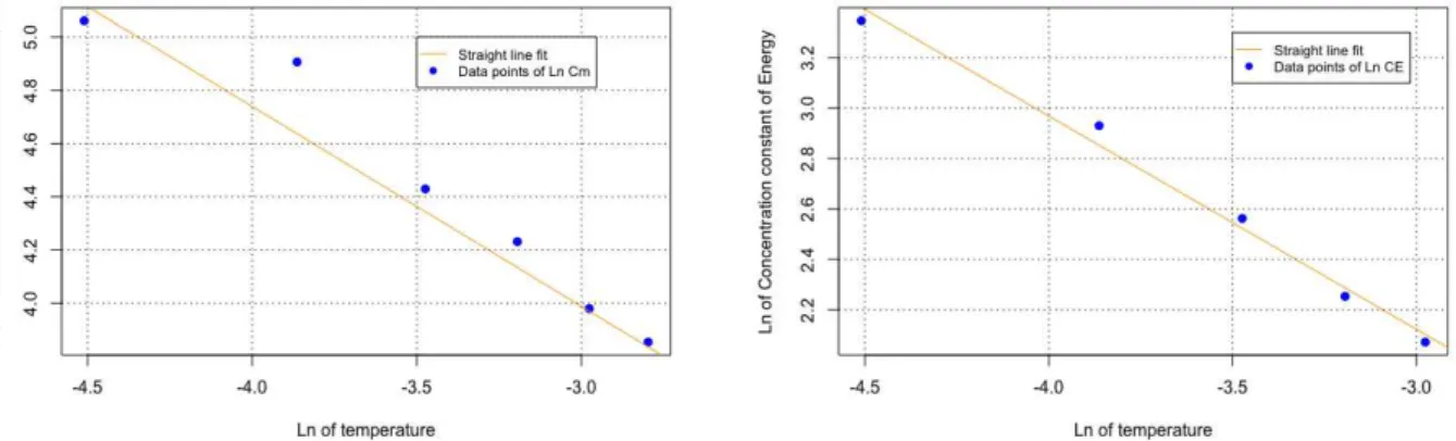
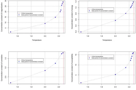
Ensuite, dans le but de clarifier le lien entre ces concepts, nous étudions num ériquement un mod èle physique particulier autorisant une transition de phase. Comme candidat naturel, nous choisissons de simuler le mod èle d’Ising ferromagn étique avec premiers voisins sans champ magn étique ext érieur en dimension deux. Nous évaluons les constantes de la concentration gr âce à la simulation d’ob-servables classiques à toute temp érature. Gr âce au comportement de ces param ètres, nous met-tons sp écialement en lumi ère le comportement de concentration Gaussienne à toute temp érature au dessus de la temp érature critique. Nous obser-vons notamment la perte de la concentration Gaus-sienne et nous analysons la divergence en loi de puissance de la constante de concentration Gaus-sienne à la temp érature critique. Dans le but de compl éter l’ étude, nous quantifions les fluctuations d’observables d’int ér êts dans le r égime des basses temp ératures dans lequel les états d’ équilibre (ou phases) ne peuvent concentrer de la m ême mani ère. Nous renforçons aussi les r ésultats th éoriques d émontr és par J-R. Chazottes, P. Collet, F. Redig ou une borne de concentration stretched-exponential a ét é prouv é pour les phases en dessous de la temp érature critique. Enfin, nous d éterminons le com-portement des constantes de concentration en fonc-tion de la temp érature.

Par la suite, motiv és par les simulations du chapitre pr éc édent, nous avons pour but de prouver que le

mod èle d’Ising ferromagn étique avec ou sans champ magn étique ext érieur en dimension deux satisfait une borne de concentration Gaussienne dans tout le r égime d’unicit é sauf à la temp érature critique lorsque h = 0. La preuve se base sur plusieurs r ésultats connus que nous devons assembler. Pour ce mod èle, nous utilisons le fait dans tout le r égime d’unicit é les mesures de Gibbs de volumes finis as-soci és au potentiel satisfont la condition de weak mixing. Ensuite, on utilise un r ésultat g én éral prouv é par F. Martinelli, E. Olivieri, and R. H. Schonmann qui dit que weak mixing est équivalent à strong mixing pour tous les carr és pour des syst èmes de spins sur r éseau en dimension deux. Cette condition implique que l’unique mesure de Gibbs en volume infini sa-tisfait une in égalit é logarithmique de Sobolev. Afin de terminer la preuve, nous prouvons que la propri ét é pr éc édente implique que l’ état d’ équilibre satisfait une borne de concentration Gaussienne.

Nous d édions un chapitre à l’ étude d’un syst ème dynamique symbolique unidimensionnel sur un al-phabet fini: les chaˆınes à liaisons compl ètes. Nous étudions en particulier les propri ét és de concentration de l’unique état d’ équilibre associ é à un potentiel (ou probabilit é de transition) non-H ölderien satisfaisant la condition de Walters. Pour des potentiels H ölderien par rapport à la distance classique ou pour des po-tentiels à variation exponentielle, nous savons qu’il existe un unique état d’ équilibre exponentiellement mixing. De plus, Jean-Ren é Chazottes et Sebastien Gouezel ont prouv é qu’il satisfait GCB. Nos r ésultats disent que GCB restent vrai pour une grande classe de potentiels φ satisfaisant la condition de Walters qui inclut la condition de variation sous-exponentielle. Enfin, nous traitons un autre syst ème dynamique important que sont les automates cellulaires pro-babilistes de voisinage fini. Cette étude aborde les automates cellulaires probabilistes comme une per-turbation d’automates cellulaires d éterministes dans un r égime de haut bruit dans lequel la mesure de Gibbs spatio-temporelle associ ée à la dynamique est l’unique mesure invariante par la dynamique et inva-riante par translation et a des propri ét és de m élange exponentiel. Dans ce contexte, nous prouvons que cette mesure satisfait aussi une borne de concentra-tion Gaussienne.

(6)

Title : On concentration inequalities for equilibrium states on lattice and symbolic dynamical systems

Keywords : Concentration inequalities, thermodynamic formalism, Gibbs measures, lattice systems, phase

transition, Ising models

Abstract : This thesis deals with concentration

pro-perties of equilibrium states for lattice systems. In the first chapter, we establish a relation between phase transitions on a general configuration space and the loss of the Gaussian concentration bound. More precisely, we show that if an equilibrium state associated to a shift-invariant and absolutely sum-mable potential satisfies a Gaussian concentration bound then it is `a fortiori mixing and unique. We prove this theorem in two different way. One uses large de-viations and the other one is a consequence of a more abstract theorem which says that if an ergodic probability measure satisfies GCB then it has the lo-wer positive relative entropy property.

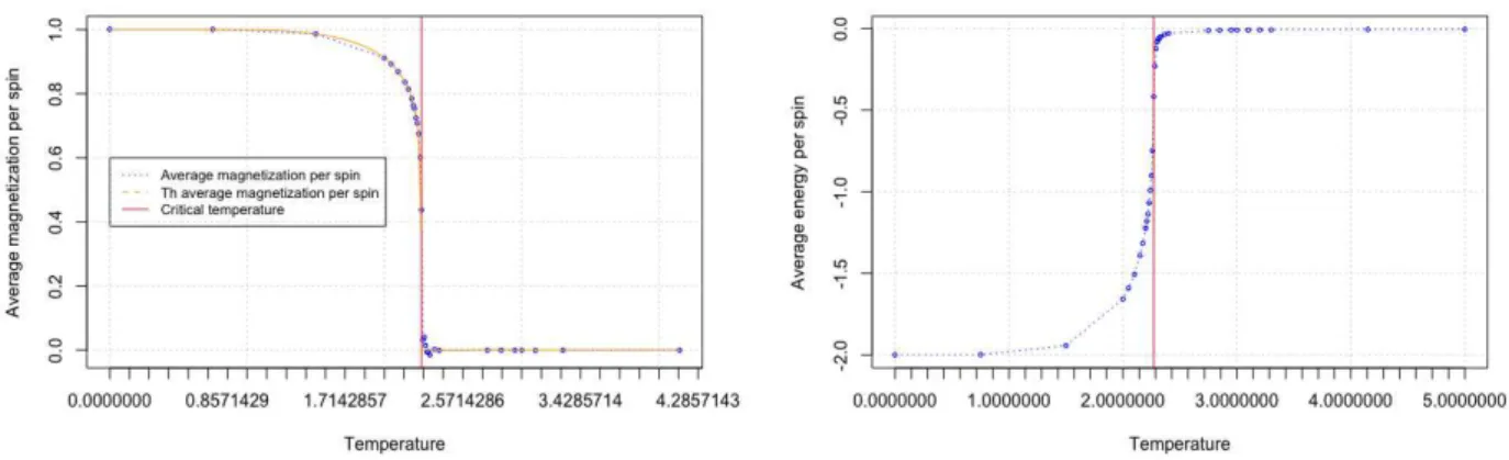
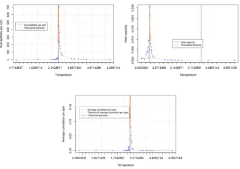
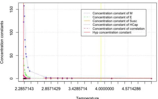
Thereafter, in view of clarifying the link between these concepts, we study numerically a particular physical model which allows phase transition to occur. As a natural candidate, we chose to compute the nearest-neighbor ferromagnetic Ising model without exter-nal magnetic field in two dimensions. We evaluate concentration constants through classical estimates at all temperatures. Thank to the behavior of these pa-rameters, at all temperatures above the critical one, we emphasize that the Gaussian concentration holds. We analyze the power-law divergence of the Gaus-sian concentration constant at the critical temperature and observe the loss of the Gaussian concentration. To complete the study, we quantify the fluctuations of observables of interest in the low-temperature regime in which the equilibrium states (or phases) cannot concentrate in the same way. We also reinforce the theoretical results proved by J-R. Chazottes, P. Collet, F. Redig where a stretched-exponential concentration bound was proven for the Gibbs measure below the critical temperature. To achieve this, we determined the behavior of the concentration parameters accor-ding to the temperature.

Later on and motivated by the simulations in the pre-vious chapter, we aim to prove that for the 2D ferroma-gnetic Ising model with or without external maferroma-gnetic

field the Gaussian concentration bound holds in the whole uniqueness regime except at the critical tem-perature when h = 0. The proof is based on several known results that we have to put together. For this model, we first use the fact that in the whole unique-ness regime the finite-volume Gibbs measures asso-ciated to the potential satisfies the weak mixing condi-tion. Then, we use a general result proved by F. Mar-tinelli, E. Olivieri, and R. H. Schonmann which says that weak mixing is equivalent to strong mixing for all squares for 2D lattice spin systems. This condition implies that the unique infinite-volume Gibbs measure satisfies a logarithmic Sobolev inequality. To com-plete the proof, we proved that the previous property implies that the equilibrium state satisfies a Gaussian concentration bound.

We dedicate a chapter to the study of an unidimen-sional symbolic dynamics on a finite alphabet: chains with complete connections. In particular, we study the concentration properties of a unique equilibrium state associated to a non-H ölderian potential (or transition probability) satisfying a Walter’s condition. For H ölde-rian potentials with respect to the classical distance or for potentials with an exponential variation, we know that there exists an exponentially mixing unique equi-librium state. Moreover Jean-Ren é Chazottes and Sebastien Gouezel proved that it satisfies GCB. Our results says that GCB remains true for a large sub-class of potentials φ satisfying Walters condition which includes the sub-exponential variation condition. Finally, we deal with another important dynamical sys-tem which is probabilistic cellular automata with finite neighborhood. This study tackles the probabilistic cel-lular automata as a perturbation of the determinis-tic cellular automata in a high noise regime in which the Gibbs measure associated to the dynamics is the unique space-time invariant shift invariant measure and has exponential mixing properties. In this context, we prove that this measure satisfies also a Gaussian concentration bound.

Institut Polytechnique de Paris

(7)

(8)

Introduction

The phenomenon we are interested in, which goes under the name of “con-centration inequalities”, is that if a function of many “weakly dependent” ran-dom variables does not depend too much on any of them, then it is concen-trated around its expected value. Among the various areas of applications (see [10, 31, 53]), it plays an important role in probability theory, statistics and for our concern in statistical mechanics. Consider independent and iden-tically distributed random variables {Êx, x œ Λn} taking values in {≠1, +1},

where Λn = [≠n, n]dﬂ Zd is the discrete cube of volume (2n + 1)d. By the

law of large numbers, the sum _(2n+1)1 d

q

xœΛnÊx converges to its expected

value (in this case 0) and its fluctuations are obviously included in an inter-val of sizeO(nd_{). In fact, by application of the well-know Hoeffding theorem,}

such an observable concentrates sharply around its mean in an interval of sizeO(nd/2_{) with high probability:}

P Q a -1 (2n + 1)d/2 ÿ xœΛn Êx --> u R b_{Æ 2 exp} A ≠u 2 2 B

for alln_{Ø 1 and for all u > 0 (see [}10]). When this bound holds, we say that the measure P satisfies a Gaussian concentration inequality.

Besides, this phenomenon doesn’t hold only for linear functions of Êx’s

(like the sum above) but for a large class of non-linear functionsF of the Êx’s.

Another interesting feature of concentration inequalities is that, unlike central limit theorems or large deviation inequalities, they are non-asymptotic. By non-asymptotic we mean that we allow the number of parameters to be large but finite.

In the general case of dependent random variables, the situation is nat-urally more complex but one may expect to have a Gaussian concentration bound as above for weakly dependent random variables Êx’s (see [64, 63,

62, 74] for the Markovian case). In this thesis, we are interested in Gibbs measures on a configuration space of the form Ω = SL

whereS is a finite

set and L = N or Zd _with _d _{Ø 1. For L = N, R. Fern´andez and G.}

Mail-lard studied the link between one-dimensional Gibbs measures associated to a potential and the generalization of Markov chains known as “chains with complete connections” (see [36]). These chains are defined by conditional probabilities of observing the next symbol which may depend on the whole “past”. In symbolic dynamics, such discrete-time stochastic processes are known as “g-measures”. Although there exist equivalence statements under some regularity conditions, in general g-measures and Gibbs measures are

(13)

not equivalent. Actually, in [34], the authors constructed a non-Gibbsian g-measure and in [7], R. Bissacot E. Endo A. van Enter and A. Le Ny identified a Gibbs measure which is not a g-measure. In this case, we adopt a dynamical system approach and we exhibit conditions for which the associated unique Gibbs measures satisfies a Gaussian concentration inequality.

We will first consider Gibbs measures on d-dimensional lattices. In the

previous example, the product measure can be identified as a Gibbs mea-sure at infinite temperature on _{{≠1, +1}}Zd

whereK is the magnetization

in-side the cube ΛnnamelyqxœΛnÊx/|Λn|. This Gaussian concentration bound

was first proved in [50] for various types of local functionK and for potentials

satisfying Dobrushin’s uniqueness condition, with a constant explicitly related to Dobrushin’s interdependence matrix. This covers, for instance, finite-range potentials at sufficiently high temperature. Not surprisingly, one cannot ex-pect that a Gaussian concentration holds for the (ferromagnetic) Ising model at temperatures below the critical one, because of the surface-order large de-viations of the magnetization (see [14] for more details). In [14], the authors proved that a “stretched-exponential” concentration bound holds for the “+” phase and the “≠” phase of this model at sufficiently low temperature. In fact, we will prove that if there exist several equilibrium states for a potential, none of them can satisfy a Gaussian concentration bound [19].

In the ferromagnetic Ising model in two dimensions, we could quantify numerically the speed with which the Gaussian concentration constant di-verges, when one approaches the critical point from above; this turns out to be a power law in the temperature. A similar behavior is found for the stretched-exponential concentration constant when one approaches the criti-cal point from below. We simulated various type of observablesK of the Êx’s

at different temperatures and estimated the concentration constant associ-ated.

This numerical study paved our way for proving that the Gaussian con-centration bound holds for all temperatures above the critical one. Let us also mention that the proof relies on different mixing properties for the Gibbs state and is only valid for finite-range discrete spin systems on the two dimensional lattice.

We will also study the concentration properties of the one-sided shift on

SN

associated to a potential satisfying Walters condition with sub-exponential continuity rates. It is well-known that when the potential is H ¨older with respect to the usual metric on the configuration space there exists a unique equi-librium state ([83,11,70]) and it satisfies a Gaussian concentration bound (see [17]). In this context, the Ruelle-Perron-Frobenius operator (or transfer operator) associated to the dynamics is quasi-compact and implies an expo-nential decay of correlations. But when the quasi-compactness doesn’t hold anymore, we obtain a sub-exponential decay of correlation which implies the existence of a unique equilibrium state (see [66]). We will prove under a summability condition on the coefficient which controls the decay of corre-lation that a Gaussian concentration bound holds for the unique equilibrium state (see [20]).

Finally, we deal with another important dynamical system which is proba-bilistic cellular automata with finite neighborhood (see [58]). This study tack-les the probabilistic cellular automata as a perturbation of the deterministic cellular automata in a high-noise regime ([52]) in which the Gibbs measure associated to the dynamics is the unique space-time invariant measure and

(14)

has exponential mixing properties. In this context, we prove that the spatio-temporal measure satisfies a Gaussian concentration bound.

(15)

(16)

Chapter 2

Setting

2.1 Configuration space

In this thesis, we are interested in models made of a configuration space of the form Ω = SL

where L= Zdwith d_{Ø 1 or L = N, and S is a non-empty}

finite set. We endow Ω with the product topology that is generated by cylinder sets. We denote by B the Borel ‡-algebra which coincides with the ‡-algebra generated by cylinder sets.

An element x of Zd _{(hereby called a site) can be written as a vector}

(x1, . . . , xd) in the canonical base of the lattice Zd. LetÎxÎŒ= max1ÆiÆd|xi|

and _ÎxÎ1 = |x1| + · · · + |xd|. If Λ is a finite subset of Zd, denote by |Λ| its

cardinality and_{diam(Λ) = max{ÎxÎ}_Œ; x_{œ Λ} its diameter.} We consider the following distance on Ω: For Ê, ÊÕ œ Ω, let

d◊(Ê, ÊÕ) = ◊k wherek = min {ÎxÎŒ: Êx ”= ÊxÕ}. (2.1.1)

where ◊ _{œ (0, 1) is some fixed number. This distance induces the product} topology and it is well-known that Ω is a compact metric space.

If Λ is a finite subset of Zd, we will write Λ b Zd. For Λ µ Zd_{, we denote}

by ΩΛthe projection of Ω onto SΛ. Accordingly, an element of ΩΛis denoted

by Ê_Λ and is viewed as a configuration Ê _{œ Ω restricted to Λ. For}σ,η œ Ω, we denote by σ_Λη_Λc the configuration which agrees withσ on Λ and with η

on Λc. We denote by B_Λ the ‡-algebra generated by the coordinate maps

Ê _{‘æ Ê}x when we restrict x to Λ. We need to define centered “cubes”: for

everynœ Z+, let

Λn= {xœ Zd:≠n Æ xi Æ n, i = 1, 2, · · · , d}.

Given Λµ Zd, an elementp_ΛofSΛ_{is called a pattern with shape Λ, or simply}

a pattern. We will write pn instead of pΛn. We will also consider elements

ofSΛ _{as configurations restricted to Λ. We will simply write Ê instead of Ê} Λ

since we will always precise to which set Ê belongs. A pattern pn œ SΛn

determines a cylinder set [pn] = {Ê œ Ω : ÊΛn = pn}. More generally, given

Λ b ZdandCµ SΛ_{, let}_{[C] = {Ê}_{œ Ω : ﬁ}

Λ(Ê)œ C} where ﬁΛis the projection

from Ω onto SΛ_.

2.2 Basics of ergodic theory

We recall basic results from [44]. We denote by M(Ω) the set of probability measures. Let us notice that since Ω is compact, then M (Ω) is also compact

(17)

in the weak topology. Recall that in this setting,(µn)nœNweakly converges to

µ if for any Λ b Zd _{and any} _C _{µ S}Λ _{one has} _µ

n([C]) æ µ([C]). We recall

that we define the shift action (Tx, x œ L) as: for each x œ L, Tx : Ω æ Ω

and(TxÊ)y = Êy≠x, for allyœ L. This is a continuous map. In fact, if L = N,

(Tx, x œ L) corresponds to the non-invertible shift map whereas, if L = Zd,

it corresponds to the invertible one. For the sake of definiteness, we take L _{= Z}d _{in the rest of this chapter. Since we will only deal with probability} measures, by “measure” we will always mean “probability measure”.

Definition 2.2.1.

A measureµœ M (Ω) is shift-invariant or translation-invariant if µ¶T≠1

x =

µ for all x_{œ Z}d, i.e., ifµ(T_x≠1A) = µ(A) for all A_{œ B. Equivalently}

’x œ Zd, ’f œ C (Ω) ⁄

f ¶ Txdµ =

⁄

f dµ

where C(Ω) is the set of real-valued continuous functions on Ω. We

denote by MT(Ω) the set of shift-invariant Borel probability measures on

Ω.

The existence of such measures is ensured by the Krylov-Bogolubov the-orem [44] which states that ifT : Ωæ Ω is continuous, then MT(Ω)”= ÿ.

We introduce some definitions for the study of measure-preserving trans-formations and their basic properties.

A measureµ _{œ M (Ω) is ergodic if µ(A) = 0 or µ(A) = 1 for all A œ B} such thatT_x≠1A = A for all xœ Zd_.

Ergodic measures are extreme points of MT(Ω) (see [27] Proposition 5.6

p. 24); we denote them by ex MT(Ω). The fundamental result in ergodic

theory is the following theorem.

Theorem 2.2.1 (Ergodic theorem,[44]).

Letµ_{œ M (Ω). For each f œ L}1_µthe limit

¯ f (Ê) := lim næŒ 1 |Λn| ÿ xœΛn f (TxÊ) (2.2.1)

exists µ-a.e. and in L1_µ. The function ¯f is T invariant and for each T -invariant setA_{µ Ω} _⁄ A ¯ f dµ = ⁄ A f dµ. (2.2.2)

Moreover, ifµ is ergodic, then

lim næŒ 1 |Λn| ÿ xœΛn f (TxÊ) = ⁄ f dµ, µ-a.e. (2.2.3)

The set of fullµ-measure such that (2.2.3) holds depends onf . However,

since Ω is compact, the space C (Ω) is separable. Hence, when µ is ergodic, there exists a measurable subset Gµ µ Ω with µ(Gµ) = 1 and such that

(18)

5.9 p. 25] for a proof.) This fact can be reformulated more compactly by using empirical measures which are defined as follows: Given Êœ Ω and any

nœ N, let E_n_{(Ê) :=} 1 |Λn| ÿ xœΛn ”_T_xÊ. (2.2.4)

Then, forµ-almost every Ê, one has

E_n_(Ê)_{≠≠≠æ µ}næŒ _(2.2.5)

where the convergence is in the weak topology on the space of probability measures M(Ω).

One important characterization of the ergodic theorem is the following.

Proposition 2.2.1 ([44]).

Forµ_{œ M (Ω) the following assertions are equivalent:} 1. µ is ergodic. 2. For allf, hœ L2 µ lim næŒ 1 |Λn| ÿ xœΛn ⁄ (f _{¶ T}x) · h dµ = ⁄ f dµ · ⁄ h dµ. (2.2.6) Definition 2.2.3 (Mixing).

A measureµœ M (Ω) is mixing if ’A, B œ B the following holds

’Á > 0, ÷n > 0, ’x œ Zd\ Λn, |µ(Tx≠1Aﬂ B) ≠ µ(A)µ(B)| < Á. (2.2.7)

Equivalently, one has

lim

ÎxÎŒæŒ

µ(T_x≠1A_{ﬂ B) = µ(A)µ(B).} (2.2.8)

Remark 2.1. An immediate consequence is that mixing implies ergodicity.

Proposition 2.2.2 ([44]).

Forµœ M (Ω) the following assumptions are equivalent:

1. µ is mixing. 2. For allf, h_{œ L}2 µ lim ÎxÎŒæŒ ⁄ (f _{¶ T}x) · h dµ = ⁄ f dµ · ⁄ h dµ. (2.2.9) 3. For allf œ L2 µ lim ÎxÎŒæŒ ⁄ (f¶ Tx) · f dµ = 3⁄ f dµ 42 . (2.2.10)

(19)

2.3 Gibbs measures and equilibrium states

We refer to [39] or [37] for details. We consider shift-invariant absolutely summable potentials. More precisely, a potential is a family of functions (Φ(Λ, ·)_ΛbZd) such that, for each (nonempty) Λ b Zd, the function Φ_Λ : Ωæ R

is B_Λ-measurable which simply means that the value of ΦΛ(Ê) is

deter-mined by Ê_Λ, the restriction of Ê to Λ. By shift-invariance we mean that Φ(Λ + x, TxÊ) = Φ(Λ, Ê) for all Λ b Zd, Ê œ Ω and x œ Zd (where Λ + x =

{y + x : y œ Λ}). Uniform summability is the property that ÿ

ΛbZd

0œΛ

ÎΦ(Λ, ·)ÎŒ<Œ. (2.3.1)

We shall denote by BT the space of shift-invariant uniformly summable

po-tentials. An important subspace of BT is the space of finite-range

poten-tials. Finite-range means that there exists R > 0 such that Φ(Λ, Ê) = 0 if

diam(Λ) > R. The smallest such R is called the range of the potential. The space of potentials of rangeR is denoted by BR, and the set of all finite-range

potentials is dense in BT.

Let Φ œ BT and Λ b Zd, the associated Hamiltonian in the finite volume

Λ with boundary condition ÷œ Ω is given by H_Λ(Ê|÷) = ÿ

ΛÕbZd

ΛÕﬂΛ”=ÿ

Φ(ΛÕ, Ê_Λ÷Zd_\Λ). (2.3.2)

The corresponding specification is defined as the family of probability kernels

“Φ = {“Φ

Λ}ΛbZd such that

“_ΛΦ(Ê|÷) = exp (≠HΛ(Ê|÷))

Z_Λ(÷) (2.3.3)

whereZ_Λ(÷) is the normalizing factor commonly called partition function in Λ. We say thatµ is a Gibbs measure for the potential Φ if “Φ

Λ(Ê|·) is a version

of the conditional probability µ(Ê_Λ|B_Λc). Equivalently, this means that for

all A _{œ B, Λ b Z}d, one has the so-called “DLR equations” (in honor of Dobrushin, Lanford and Ruelle)

µ(A) =

⁄

dµ(÷) ÿ

ÊÕ_œSΛ

“_ΛΦ(ÊÕ|÷)1A(ÊÕ_Λ÷Λc). (2.3.4)

We denote by G(Φ) the set of Gibbs measures for a given absolutely summable potential Φ. This set is never empty, but it may be not reduced to a singleton. LetGT(Φ) = G(Φ)ﬂ MT(Ω), that is, the set of shift-invariant

probability measures for Φ. This set is a Choquet simplex and may con-tain several (extremal) elements. We denote byex GT(Φ) the set of extreme

points which coincides with the set of ergodic Gibbs measures for Φ, that is, ex GT(Φ) = GT(Φ)ﬂ ex MT(Ω). Of course, when G(Φ) is a singleton, then the

unique Gibbs measure is shift-invariant and ergodic.

We now define relative entropy. Letµ, ‹ œ MT(Ω). For each nœ N, let

Hn(‹|µ) := ÿ pnœSΛn ‹([pn]) log ‹([pn]) µ([pn]) .

(20)

Let µ, ‹ œ MT(Ω). The lower and upper relative entropies of ‹ with

respect toµ are defined by

h_ú(‹|µ) = lim inf næŒ Hn(‹|µ) (2n + 1)d, hú(‹|µ) = lim sup_n æŒ Hn(‹|µ) (2n + 1)d. (2.3.5)

When the limit exists, we puth(‹|µ) = h_ú(‹|µ) = hú(‹|µ).

It is well known that h_ú(‹|µ) and hú_{(‹|µ) are non-negative numbers. Note}

that Hn(‹|µ) can be +Œ if µ([pn]) = 0 for some pn but this will not happen

whenµ is fully supported. Let Φœ BT andµœ G(Φ). It is proved in [39] that

for any ‹ œ MT(Ω) we have

h_ú(‹|µ) = hú(‹|µ) = h(‹|µ) = P (Φ) +ÿ

0œΛ

|Λ|≠1 ⁄

Φ(Λ, ·)d‹≠ h(‹) (2.3.6)

whereh(‹) is the entropy of ‹ and P (Φ) is the pressure of Φ defined as follows h(‹) := lim næŒ≠ 1 (2n + 1)d ÿ pnœSΛn ‹([pn]) log ‹([pn]) P (Φ) := sup ‹œMT(Ω) Q ah(‹) +ÿ 0œΛ |Λ|≠1 ⁄ Φ(Λ, ·)d‹ R b.

Notice that, ‹ œ MT(Ω), h(‹|µ) is the same number for all µœ GT(Φ), so

it is natural to define, for each ‹ _{œ M}T(Ω),

h(‹|Φ) := h(‹|µ) whereµ is any element in GT(Φ).

We recall the definition of equilibrium states.

Definition 2.3.2 (Equilibrium states).

Let Φœ BT. A shift-invariant probability measure ‹ such thath(‹|Φ) = 0

is called an equilibrium state for Φ.

We have the following fundamental result which is usually referred to as the variational principle for equilibrium states (see [39], Chapter 15, [72],Theorem 4.2).

Theorem 2.3.1 (Variational principle).

Let Φœ BT. We haveh(‹|Φ) = 0 if and only if ‹ œ GT(Φ). In particular,

GT(Φ) coincides with the set of equilibrium states for Φ.

Nearest-neighbor Ising model. First consider the nearest-neighbor ferro-magnetic Ising model (S = {_{≠1, +1}) with d Ø 2:}

Φ(Λ, Ê) = Y _ _ ] _ _ [ ≠hÊx if Λ = {x} ≠JÊxÊy if Λ = {x, y} andÎx ≠ yÎ1 = 1 0 otherwise (2.3.7)

(21)

whereJ, h _{œ R represents respectively the interaction strength and the}

ex-ternal magnetic field. We will always assume thatJ > 0 (the ferromagnetic

case of the Ising model). Consider the potential —Φ where — œ R+ is the

inverse temperature and the Gibbs measures µ+_—Φ and µ≠_—Φ obtained as the infinite-volume limits of the corresponding specification with “+” and the “_≠” boundary conditions, respectively. There exists —c = —c(d) > 0 such that, if

— < —c then it is well-known that µ—Φ = µ+—Φ = µ≠—Φ is the unique ergodic

Gibbs measure and if — > —c then µ+_—Φ and µ≠_—Φ are distinct ergodic Gibbs

measures. Ford = 2, for all — > —c,GT(—Φ) = {⁄µ+_—Φ+ (1≠ ⁄)µ≠_—Φ: ⁄œ [0, 1]}

(henceex GT(—Φ) = {µ+_—Φ, µ≠_—Φ}).

Long-range Ising model. Consider the long-range Ising model whereS =

{≠1, +1}, d = 1, and Φ(Λ, Ê) = Y ] [ ≠ ÊxÊy

|x≠y|– if Λ = {x, y} such that x”= y

0 otherwise

with – > 1. If 1 < – Æ 2 then, there exists —c > 0 such that, for all — < —c,

µ+_—Φ _{”= µ}≠_—Φ and ex G(—Φ) = {µ+_—Φ, µ≠_—Φ}. We refer to [68] for the relevant references.

Potts model. Consider the nearest-neighbor Potts ferromagnet model for whichS = {1, · · · , N } for sufficiently large N _{œ N:}

Φ(Λ, Ê) = I

J1Êx=Êy if Λ = {x, y} andÎx ≠ yÎ1= 1

0 otherwise

whereJ > 0 is the interaction strength. There exists 0 < —N < +Œ such that

|ex G(—NΦ)| = N + 1, one of these measures being symmetric under spin flip,

|ex G(—Φ)| = N when — > —N and when —< —N,|ex G(—Φ)| = 1.

Dobrushin’s uniqueness regime. Let Φœ BT and “Φ be the

correspond-ing specification. One says that “Φ _{satisfies Dobrushin uniqueness condition}

if c(“Φ) := ÿ xœZd C0,x(“Φ) < 1 (2.3.8) where Cx,y(“Φ) := sup Ó Î“Φ

{x}(·|Ê)≠ “{x}Φ (·|ÊÕ)ÎŒ: Ê, ÊÕ differ only at sitey

Ô

.

Under this abstract condition valid in more general cases, there exists a unique equilibrium state for Φ which we denote by µΦ (see [39], chapter 8

and [14]). An interesting sufficient condition for2.3.8to hold is that ÿ 0œΛ (|Λ|≠ 1)”(Φ(Λ, ·)) < 2 (2.3.9) where ”(Φ(Λ, ·)) = sup Ê,ÊÕ_œΩ|Φ(Λ, Ê) ≠ Φ(Λ, Ê Õ_)|.

Condition (2.3.9) is satisfied by any finite-range potential —Φ provided that

(22)

sufficiently small (high-temperature regime of the potential), we observe that

“—Φ satisfies Dobrushin uniqueness condition.

We now consider any potential such that Φ({x}, Ê) =≠hÊx for allxœ Zd

and h _{œ R (external magnetic field). If h is sufficiently large, then}2.3.9 also holds. In fact the condition implying2.3.9reads

exp Q a1 2 ÿ 0œΛ:|Λ|>1 ”(Φ(Λ, ·)) R bÿ 0œΛ (|Λ|≠ 1)”(Φ(Λ, ·)) < e|h|.

Finally, one can also check that this condition holds at low temperatures for potentials with unique ground state , e.g., the nearest-neighbor Ising model with non zero external magnetic field and sufficiently large —, or for large enough|h| and for all —.

(23)

(24)

Chapter 3

Concentration inequalities

3.1 Basics of concentration inequalities

We start by reviewing elementary facts about concentration inequalities. Let (X , A, P) be a probability space. We give several well-known inequalities to estimate how a real-valued random variable X deviates from its expected

value E(X) , i.e., on how we can bound P(X_{≠ E(X) Ø u) and P(X ≠ E(X) Æ} ≠u) depending on the deviation u > 0.

An elementary but powerful device to quantify tail probabilities is Markov’s inequality.

Theorem 3.1.1 (Markov’s inequality).

LetZ be a non-negative real-valued random variable and suppose that

E(Z) < +_{Œ. Then,}

’u > 0, P(Z Ø u) Æ E(Z)

u . (3.1.1)

A classical and easy improvement of this inequality can be achieved under stronger integrability conditions onZ as follows.

Corollary 3.1.1.

Let „ be a non-negative and non-decreasing function defined on an in-terval I _{µ R and Z a real-valued random variable taking values in I.} Then,

’u > 0, P(Z Ø u) Æ E(„(Z))

„(u) . (3.1.2)

Chebyshev’s inequality follows directly from this corollary by taking „(u) =

u2 _and_{Z = |X}_{≠ E(X)|:}

’u > 0, P(|X ≠ E(X)| Ø u) Æ Var(X)_u₂ .

This result applies in various cases requiring weak properties of random vari-ables and it is a sufficient condition to prove for instance the weak law of large numbers. For example, let’s consider independent and identically dis-tributed random variables(Xi)1ÆiÆn andZ = X1+ · · · + Xn≠ nE(X1) such

(25)

thatVar(X1) < +Œ. In this case, Chebyshev’s inequality becomes PA--- -1 n n ÿ i=1 Xi≠ E(X1) --Ø u B Æ ‡ 2 nu2. where ‡2 _{= Var(X}

1). If one can prove the existence of moments of higher

order p > 2, then by setting „(u) = up, we would have a better estimate, namely

P_(|Z_{≠ E(Z)| Ø u) Æ} E(|Z≠ E(Z)|

p₎

up , u > 0.

If the random variable Z is such that E(|Z|p) < +_{Œ for all p > 0, then one} may choose the value ofp which optimizes the upper bound. One can get an

improvement by using „(u) = e⁄u where ⁄ > 0. This is known as Chernoff’s

bounding method.

Proposition 3.1.1 (Chernoff’s inequality).

LetZ be a real-valued random variable such that E(e⁄Z_{) < +}_{Œ for all}

⁄> 0. Then, for all u > 0

P_(Z_{Ø u) Æ e}≠⁄uE_(e⁄Z_). _(3.1.3) Hoeffding inequality is an application of Chernoff’s inequality for sums of independent bounded random variables.

Theorem 3.1.2 (Hoeffding’s inequality).

Let n Ø 1 and (Xk)1ÆkÆn be a sequence of independent real-valued

random variables such that, for all sequences (ak)1ÆkÆn, (bk)1ÆkÆn of

real numbers withak< bkfor allkÆ n, we have

’k, P(akÆ XkÆ bk) = 1. (3.1.4) Letting Sn= n ÿ k=1 Xk (3.1.5)

we have, for allu > 0,

P_(S_n_{≠ E(S}_n_{) > u)}_{Æ exp} A ≠ 2u 2 qn k=1(bk≠ ak)2 B , (3.1.6)

P_(S_n_{≠ E(S}_n_{) <}_{≠u) Æ exp} A ≠ 2u 2 qn k=1(bk≠ ak)2 B , (3.1.7) P_(|S_n_{≠ E(S}_n_{)| > u)}_{Æ 2 exp} A ≠ 2u 2 qn k=1(bk≠ ak)2 B . (3.1.8)

Subsequently, Hoeffding and Azuma proved that the following general-ization holds for martingales with bounded differences. Given a filtration F = (F0 = {Ω,ÿ} µ F1 µ · · · µ Fn), let Z be a Fn-measurable real-valued

(26)

reverse martingale differences, i.e., Z≠ E[Z] = n ÿ i=1 Di (3.1.9) where Di= E[Z|Fi]≠ E[Z|Fi≠1]. (3.1.10)

Let’s definedi := supiDi≠ infiDi. We have the following result.

Theorem 3.1.3 (Azuma-Hoeffding inequality).

LetZ be a martingale with respect to a filtration F = (F0 = {X ,ÿ} µ

F1 µ · · · µ Fn). Then, for all ⁄œ R,

E_{[exp (⁄(Z}_{≠ E(Z)))] Æ exp} A ⁄2 8 n ÿ i=1 d2_i B . (3.1.11)

In particular, for allu > 0,

P_(|Z_{≠ E(Z)| > u) Æ 2 exp} A ≠ 2u 2 qn k=1d2i B . (3.1.12)

Remark 3.1. One can always bound|di| by 2ÎDiÎŒ.

This Gaussian inequality has paved the way for the study of more general functions than the sum of bounded random variables. The first step was real-ized by McDiarmid who generalreal-ized Hoeffding’s inequality3.1.2 considering sufficiently “smooth” functions of independent random variables.

Theorem 3.1.4 (McDiarmid’s inequality).

Letn _{Ø 1, (X}k)1ÆkÆn be a sequence of independent random variables

taking values in some spaceX and K : Xn _{æ R be a function. Assume}

that there exists nonnegative constants ¸iwith1Æ i Æ n such that for all

x1, · · · , xn, xÕiœ X , one has

|K(x1, · · · , xi, · · · , xn)≠ K(x1, · · · , xÕi, · · · , xn)|Æ ¸i.

Then, for all ⁄_{œ R,}

E_{[exp (⁄(K(X}₁_{, · · · , X}_n₎_{≠ E[K(X}₁_{, · · · , X}_n_)]))]_{Æ exp} A ⁄2 8 n ÿ i=1 ¸2_i B .

In particular, for allu > 0,

P_(|K(X₁_{, · · · , X}_n₎_{≠ E[K(X}₁_{, · · · , X}_n_{)]| > u)}_{Æ 2 exp} A ≠ 2u 2 qn k=1¸2i B .

Remark 3.2. The regularity condition onK known as the bounded difference property makes possible the application of McDiarmid’s inequality to non-bounded random variables.

Inequality 3.1.4 is the prototype of what we are going to call Gaussian concentration bound.

(27)

Beyond the independent case, Markov chains were considered by K. Mar-ton [62, 63, 64] and by P-M. Samson [74] where Gaussian concentration bounds hold. We also refer to the book of R. Douc, E. Moulines, P. Priouret and P. Soulier [30] for further details. Another setting where people proved Gaussian concentration bounds for partially Lipschitz functions are hyperbolic dynamical systems [17]. They showed that for sufficiently mixing invariant measures, GCB holds. In particular, for Young towers, they deduced Gaus-sian/polynomial concentration from the tails of the return time on the basis of the tower.

In this thesis, we will pay attention to the dependent aspect of bounded random variables distributed according to Gibbs measures. Indeed, we will discard the unbounded aspect of random variables where GCB may not hold even for sums. One of our motivations is to understand the loss of the Gaus-sian concentration bound when the random variables become highly depen-dent (for example in low temperature Ising model where we can’t control uni-formly_ÎDiÎŒbecause of the correlations).

3.2 Known results for Gibbs measures

Recall that Ω = SZd

whereS is a finite set. In this context, let K : Ωæ R be a continuous function andx_{œ Z}d_{. The oscillation of}_{K at x is defined by}

”x(K) = sup {|K(Ê)≠ K(ÊÕ)| : Ê, ÊÕ œ Ω differ only at site x}.

This is a quite natural object since, given Λ b Zd and two configurations

Ê, ÷_{œ Ω such that Ê}_Λc = ÷_Λc, one has

|K(Ê) ≠ K(÷)| Æ ÿ

xœΛ

”_x(K) 1{Êx”=÷x}.

We shall say that K : Ω æ R is a local function if there exists Λ b Zd (the dependence set ofK) such that for all Ê,Ê,Â Ê‚,K(Ê_ΛÊÂ_Λc) = K(Ê_ΛÊ‚_Λc). (This

means that K is B_Λ-measurable.) Equivalently, this means that ”x(K) = 0

for allx /_{œ Λ. It is understood that Λ is the smallest such set. Local functions}

are continuous, hence bounded. (In fact, continuous functions are obtained as uniform limits of local functions.)

We writeδ(K) for the infinite array (δx(K), xœ Zd), and let

Îδ(K)Î22 :=Îδ(K)Î2¸2_(Zd₎=

ÿ

xœZd

δx(K)2.

It is convenient to define the following set of all local functions. Let

L ₌ €

ΛbZd

L_Λ _(3.2.1)

where L_Λ is the set of local functions whose dependence set is Λ.

3.2.1 Gaussian concentration bound

(28)

Definition 3.2.1 (Gaussian concentration bound).

Let µ be a probability measure on (Ω, B). We say that µ satisfies a Gaussian concentration bound if there existsD = D(µ) > 0 such that, for all functionsK_{œ L , we have}

E_µ#_{exp (K}_{≠ E}_µ_[K])$_{Æ exp}1_D_Î”(K)Î2₂2_. _(3.2.2)

For the sake of brevity, we say thatµ satisfies GCB(D).

We denote by Eµ the expectation with respect to µ. A key point in this

defi-nition is thatD is independent of K, in particular it is independent of the size

of the dependence set ofK. Inequality (3.2.2) easily implies the following tail inequality that we will use several times.

Proposition 3.2.1.

If a probability measureµ on (Ω, B) satisfies GCB(D) then, for all K œ L

and for allu > 0,

µ)Ê _{œ Ω : K(Ê) Ø E}µ[K] + u*Æ exp A ≠ u 2 4DÎ”(K)Î2 2 B . (3.2.3)

Proof. IfK œ L then, for any ⁄ > 0, ⁄K obviously belongs to L . Applying Markov’s inequality and (3.2.2) we get

µ {Ê_{œ Ω : K(Ê) ≠ E}µ[K]Ø u} Æ exp (≠⁄u) Eµ#exp (⁄(K≠ Eµ[K]))$

Æ exp1≠⁄u + DÎ”(K)Î22⁄2

2

.

Minimizing over ⁄ yields (3.2.3).

Thus, looking for a Gaussian concentration bound consists in finding the existence of a strictly positive constantD satisfying (3.2.2). In practice, get-ting the optimal constant is out of reach.

Proposition 3.2.2.

If a probability measureµ on (Ω, B) satisfies GCB(D), then it satisfies the variance inequality

Varµ(K) := Eµ[K2]≠ (Eµ[K])2Æ 2DÎ”(K)Î22 (3.2.4)

for all functionsKœ L.

The proof goes roughly as follows, the details are left to the reader. Take

⁄> 0 and apply (3.2.2) to ⁄K, subtract 1 on both sides and divide out by ⁄2

the resulting inequality. Then (3.2.4) follows easily by Taylor expansion and letting ⁄ tend to0.

Now, let’s give some examples.

Dobrushin’s uniqueness regime. The following theorem ensures that a Gaussian concentration bound holds under Dobrushin uniqueness condition

(29)

Theorem 3.2.1 (GCB under Dobrushin’s uniqueness condition).

Let Φ œ BT and assume that the associated specification “Φ satisfies

Dobrushin’s uniqueness condition2.3.8. Thenµ_ΦsatisfiesGCB(D) with

D = (2(1_{≠ c(“}Φ₎₎2₎≠1_.

This holds for instance for any finite-range potential —Φ provided that

— > 0 is small enough. As a basic example, we mention the nearest-neighbor

ferromagnetic Ising model without magnetic field at sufficiently high tempera-ture which is such that there exists ¯— < —c such that for all — < ¯—, one has,

for allK _{œ L and for all u > 0}

µ_—Φ)Ê _{œ Ω : K(Ê) Ø E}µ—Φ[K] + u * Æ exp A ≠(1≠ tanh —J) 2_u2 2Î”(K)Î2 2 B .

Note that a Gaussian concentration bound does not only hold at high-temperature regime but it can also hold at sufficiently low-high-temperature regime with sufficiently large external magnetic field (see2.3and [14] for more details and examples). We will prove in chapter6that, in dimension two, we have a Gaussian concentration bound for all —< —c.

Remark 3.3 (The 2D Ising model at — = —c.).

It is known (see [[33] p. 172]) that for — = —c = log (1 +Ô2)/2, there is a

unique Gibbs measureµ—c such that

lim næŒ 1 Λn Varµ_—c Q aÿ xœΛn Êx R b= +_Œ. (3.2.5)

Therefore, µ—c cannot satisfy a Gaussian concentration bound because, by (3.2.4), one would have

lim sup næŒ 1 Λn Varµ_—c Q aÿ xœΛn Êx R b_{Æ 8D} (3.2.6)

which contradicts (3.2.5). To obtain (3.2.6), apply (3.2.4) to K(Ê) = ÿ

xœΛn

ﬁ_{0}(TxÊ),

where ﬁ_{0}(Ê) = Ê0. Then use Lemma4.1.1to get

Varµ_—c Q aÿ xœΛn Êx R b_{Æ 8D|Λ}_n|

for alln. Therefore, the Gibbs measure for the Ising model in dimension 2 at critical temperature does not satisfy a Gaussian concentration bound. It does not even satisfy the variance inequality (3.2.4).

Now, we give some applications and refer the reader to [14] for more details and more applications.

(30)

Empirical magnetization The magnetization is of particular interest in the context of Gibbs measures. Let Λ b Zd, we define the empirical magnetiza-tion in Λ by

M_Λ(Ê) =ÿ

xœΛ

Êx.

We have the following theorem.

Theorem 3.2.2 ([14]).

Dobrushin’s uniqueness condition2.3.8. Then, for all Λ b Zd, we have

µ_Φ 3 Ê_{œ Ω :} -M_Λ(Ê) |Λ| ≠ EµΦ[Ê0] --Ø u 4 Æ 2 exp A ≠(1≠ c(“Φ)) 2 8 |Λ|u 2 B .

Speed of convergence of the empirical measure. The aim is to quantify the speed of convergence of empirical measures in2.2.5. We endow M(Ω) with the Kantorovich distancedKdefined by

dK(µ1, µ2) = sup {Eµ1[G]≠ Eµ2[G] : G : Ωæ R such that G 1-Lipshitz} .

A function G : Ω æ R is 1-Lipschitz if |G(Ê) ≠ G(ÊÕ_)| _{Æ d(Ê, Ê}Õ_{) where the}

distanced(·, ·) is defined in 2.1.1. Theorem 3.2.3 ([14]).

Dobrushin’s uniqueness condition2.3.8. Denote byµ_Φ the correspond-ing Gibbs measure. Then

µ_Φ1Ê_{œ Ω :}--dK(En(Ê), µΦ)≠ EµΦ[dK(En(·), µΦ) ] --_{Ø u}2 Æ 2 exp A ≠(1≠ c(“Φ)) 2 2cd |Λn|u 2 B

for alln _{Ø 1 and for all u > 0, where c}dis a constant only depending on

d.

Remark 3.4. For convenience, we decided to deal with empirical measures

on “cubes” but this theorem remains valid for all Λ b Zd.

Bounding ¯d-distance by relative entropy. Given nœ N, we define the non normalized Hamming distance between Ê and ÊÕ in Ωnby

¯ dn(Ê, ÊÕ) = ÿ xœΛn 1_Ê x”=ÊxÕ.

Letµ, ‹ _{œ M}T(Ω) and define the ¯d-distance as follows.

¯ d(µn, ‹n) = inf P_n_œJ_T_(µ_n_,‹_n₎ ⁄ Ωn ⁄ Ωn ¯ dn(Ê, ÊÕ)dPn(Ê, ÊÕ)

whereJT(µn, ‹n) denotes the set of all shift-invariant couplings of µnand ‹n.

By [73], it follows that ¯d(µn, ‹n) normalized by (2n + 1)d converges to a limit

(31)

Theorem 3.2.4 ([14]).

Dobrushin’s uniqueness condition 2.3.8. Then for every shift-invariant probability measure ‹ ¯ d(µ_Φ, ‹)_Æ Ô 2 1≠ c(“Φ₎ Ò h(‹|µ_Φ).

3.2.2 Moment concentration bounds

For the Ising model (dØ 2) without external magnetic field, at sufficiently low temperature, one cannot expect Gaussian concentration inequalities because it would contradict the “surface-order” large deviation for the magnetization. However, the authors of [13] showed that one can control all moments and deduce that moment concentration bounds hold. We give the general form of such bound.

Definition 3.2.2 (Moment concentration bound).

Letµ be a probability measure on (Ω, B). Given p œ N, we say that µ

satisfies a moment concentration bound of order2p with constant C2p=

C2p(µ) > 0 (abbreviated MCB(2p,C2p)) if, for all functionKœ L , we have

E_µ#_(K_{≠ E}_µ_[K])2p$_{Æ C}_2p_Î”(K)Î2₂_. _(3.2.7) In the same vein as the proposition3.2.1, we have for allu > 0

µ)Ê_{œ Ω : |K(Ê) ≠ E}µ[K]|Ø u*Æ

C2pÎ”(K)Î2p2

u2p . (3.2.8)

Theorem 3.2.5 ([13,14]).

Let µ+_—Φ be the plus-phase of the low-temperature Ising model. There exists ¯— > —c, such that for each — > ¯—, there exists a positive sequence

(C2p(—))pœNsuch thatµ+—Φsatisfies MCB(2p,C2p(—)) for all pœ N.

For this model, one may wonder whether the previous theorem implies a stronger statement like a Gaussian concentration bound. In fact, one cannot infer a Gaussian concentration bound because C2p is of the formp2pGp for

some constantG > 0 depending on K but not of p (see Theorem 3 in [13,

14]). For someC2pwhich does not “grow too fast”, Gaussian concentration is

equivalent to moment concentration for allp_{œ N (see [}10]).

3.2.3 Stretched-exponential concentration bound

For the Ising model at sufficiently low temperature, it turns out that the control of all moments leads to a stretched-exponential concentration bound which we define as follows. Let0 < ﬂ < 1 and define the Young function by Mﬂ :

R_{æ R}+_{such that for all}_x_{œ R}

Mﬂ(x) := e(|x|+hﬂ)

ﬂ

(32)

wherehfl= 1 1≠fl fl 21 fl

. We also define the Luxemburg norm with respect toMﬂ

of a real-valued random variableK as

ÎKÎMﬂ = inf ; ⁄> 0 : E 5 Mﬂ 3_K ⁄ 46 Æ 1 < .

Let us mention that the set of all functionsK : Ωæ R such that ÎKÎMﬂ< +Œ

is called a Orlicz space. These spaces generalizeLp_µspaces.

Definition 3.2.3 (Stretched-exponential concentration bound).

Letµ be a probability measure on (Ω, B). Given p œ N, we say that µ

satisfies a stretched-exponential concentration if there exists fl= fl(µ)_œ (0, 1) and a constant Dfl> 0 (abbreviated SECB(fl,Dfl)) such that, for all

functionK _{œ L , we have}

ÎK ≠ Eµ[K]ÎMﬂ Æ DﬂÎ”(K)Î2. (3.2.9)

This general definition leads to the following proposition.

Proposition 3.2.3 ([13]).

If a probability measure µ on (Ω, B) satisfies SECB(ﬂ,Dﬂ) then there

existsCﬂsuch that for all functionKœ L and for all u > 0,

µ)Ê_{œ Ω : |K(Ê) ≠ E}µ[K]|Ø u*Æ 4 exp 3 ≠ Dflu fl Î”(K)Îfl2 4 . (3.2.10) For the plus-phase of the low temperature Ising model, we mention the theorem in [13,14].

Theorem 3.2.6 ([13,14]).

Let µ+_—Φ be the plus-phase of the low-temperature Ising model. There exists ¯— > —c, such that for each — > ¯—,µ+_—Φsatisfies SECB(ﬂ,Dﬂ).

It is unlikely that the dependence ofu is optimal. The constants ﬂ and Dﬂ

appearing in this theorem are not explicit and depend on the dimensiond and

the temperature. As a matter of fact, let considerK : Ωæ R as the empirical magnetization in Λ, then one has the following.

Theorem 3.2.7 ([13,14]).

Let µ+_—Φ be the plus-phase of the low-temperature Ising model. There exists ¯—> —c, such that for each — > ¯—, there exist ﬂ= ﬂ(—)œ (0, 1) and

a constantDﬂsuch that for all Λ b Zd, we have

µ+_— 3 Ê_{œ Ω :} -M_Λ(Ê) |Λ| ≠ Eµ+_—[Ê0] --Ø u 4 Æ 4 exp 3 ≠Dfl 2fl|Λ| fl 2ufl 4 .

At low temperature, one has “surface-order” large deviations (see [76]). In particular, leta, b such that

≠E_µ+

—[Ê0] < a < b < Eµ

+

(33)

then the probability (under µ+_—) that M_Λn/|Λn| falls into an interval [a, b] is

exponentially small in(2n + 1)d≠1_{, as}_{n goes to infinity. This result is actually}

sharper than the stretched-exponential bound (since ﬂd/2 < d≠1 for all d Ø 2) which is valid in any finite volume and for a large class of functions. Later, we will investigate numerically this behavior.

3.3 Known results for stochastic chains of unbounded

memory (SCUMs)

In view of Chapter 7, we give recent results on concentration inequalities for SCUMs which are a natural generalization of Markov chains by consider-ing the whole “past”. In the literature on stochastic processes, SCUMs are also known as “chains with complete connections”. Such one-dimensional systems are simultaneously studied as discrete-time processes in symbolic dynamics under the name of “g-measures” and as Gibbs measures on the lattice N or Z associated to a family of specifications. For further details, we refer the reader to R. Fern ´andez and G. Maillard [36] and S. Berghout, R. Fern ´andez and E. Verbitskiy [6] where they study the similarities and the dif-ferences between these different objects. Let Ω = SN

whereS is a finite set.

We consider the following class of functions. Letn_{œ N and K : S}n_{æ R, and}

let

”_j(K) = sup

aj=bj,’j”=i

{|K(a0, . . . , ai, . . . , an≠1)≠ K(b0, . . . , bi, . . . , bn≠1)|} .

(3.3.1) Now letK : Snæ R and

Îδ(K)_Î2₂ :=

+Œ

ÿ

j=≠Œ

δj(K)2 (3.3.2)

whereδ(K) is the column vector of size n whose j-th coordinate is ”j(K). We

stress that this class of functions is analoguous to thed-dimensional case.

We will say that a measureµ on (Ω, B) satisfies a Gaussian concentration

bound if it satisfies 3.2.1 for all n _{œ N and K : S}n _{æ R. This statistical}

property is derived from the control of the dependence of the past of the probability transitions quantified by either the variation or the oscillation (see [38,16]). Here, we will only mention the variation of a kernel/potential defined as follows:

varn(„) := sup{|„(x)≠ „(y)| : xi = yi, 0Æ i Æ n ≠ 1}.

In [38], the authors proved a Gaussian concentration bound for poten-tials with summable variations. Recently, J.R Chazottes, S. Gallo and D. Takahashi have generalized the previous result obtaining optimal Gaussian concentration bounds for chains with complete connections on a countably infinite alphabet. Their proofs rely on maximal coupling techniques and on the tight control of the summability of its variations (see [16]).

In Chapter7, we will obtain Gaussian concentration bounds for separately Lipschitz functions on Ωn_{. To do so, we use the spectral properties of}

Ruelle-Perron-Frobenius’ operator associated to the potential and, in particular its speed of convergence to the unique equilibrium state for Lipschitz observ-ables. Of course, this result also holds for allK : Sn _{æ R. We will deduce}

(34)

3.4 On the relation between concentration and large

deviations for equilibrium states

We refer to [82] for more details and references on large deviations. An in-teresting consequence is that it provides a statistical interpretation of relative entropy2.3.5(see [82]). We will briefly explain the differences between Gaus-sian concentration bounds and large deviations.

First, let’s consider equilibrium states for Φ, µ œ GT(Φ) and local

observ-ablesK : Ωæ R. We define the Birkhoff sum of K as

S_nK := ÿ

xœΛn

K¶ Tx.

Then, by Theorem 2.2.1, S_nK/|Λn| converges in probability to the expected

valuesKdµ. This can be reformulated as follows: If I is a closed interval of

R_{which does not contain}s _{Kdµ then} lim næŒµ I Ê_{œ Ω :} S K n(Ê) |Λn| œ I J = 0.

The aim of large deviations theory is to strengthen the ergodic theorem in the sense that it gives asymptotically the precise rate of convergence of this probability on the logarithmic scale. Let Ê _{œ Ω and K œ L , then the large} deviation principle states that for all closed intervalI of R

lim sup næŒ 1 |Λn| log µÓÊ_{œ Ω :}S K n (Ê) |Λn| œ I Ô Æ ≠ inf ; h(‹|µ) : ‹ _{œ M}T(Ω) with ⁄ Kd‹ _{œ I} <

and for all open intervalsI of R

≠ infÓh(‹|µ) : ‹ _{œ M}T(Ω) with ⁄ Kd‹ _{œ I}Ô Æ lim inf_n_æŒ 1 |Λn| log µ I Ê _{œ Ω :} S K n(Ê) |Λn| œ I J .

We can formulate a more abstract large deviation principle on the level of empirical measures(En)nœN (2.2.4). For all subsetsA µ M (Ω) which do not

containµ, if A is a closed set then

lim sup

næŒ

1 |Λn|

log µ{Enœ A} Æ ≠ inf {h(‹|µ) : ‹ œ A ﬂ MT(Ω)} (3.4.1)

and ifA is an open set then

≠ inf {h(‹|µ) : ‹ œ A ﬂ MT(Ω)}Æ lim inf_n

æŒ

1 |Λn|

log µ{Enœ A}. (3.4.2)

If we consider µ as a product measure, the events{En œ A} are sufficient

to describe completely the measure. In the case of Gibbs measures, one needs observables which depends on a large number of sites to describe the dependence in between. Then, the large deviation principle describes the relative entropy in terms of rate functions, i.e., the probability that a configu-ration Ê distributed according toµ looks like a typical configuration from ‹ in

On concentration inequalities for equilibrium states in lattice and symbolic dynamical systems

HAL Id: tel-03152537

https://tel.archives-ouvertes.fr/tel-03152537

On concentration inequalities for equilibrium states in

lattice and symbolic dynamical systems

Jordan Moles

To cite this version:

NNT

:

2020IPP

AX102

On concentration inequalities for

equilibrium states in lattice and symbolic

dynamical systems

J

M

Acknowledgements

Contents

Chapter 1

Introduction

Chapter 2

Setting

2.1

Configuration space

2.2

Basics of ergodic theory

2.3

Gibbs measures and equilibrium states

Chapter 3

Concentration inequalities

3.1

Basics of concentration inequalities

3.2

Known results for Gibbs measures

3.3

Known results for stochastic chains of unbounded

memory (SCUMs)

3.4

On the relation between concentration and large

deviations for equilibrium states