Codon and aminoacid usage in bacteria (Haeckel, 1874)

(1)

(Haeckel, 1874)

P

r

_{Jean R. Lobry}

Work in progress. This is release : June 10, 2019

Pre-α release tag

(2)

(3)

W

arning: this is not a peer-reviewed nor a genuine published piece of work. This is just a draft, a work in progress. I’m planning to have an α-version for spring 2020, a β-version for spring 2021, and hopefully a decent version in spring 2022. In the meantime, feedback is more than welcome. Just look for the string “jean lobry” in your favorite internet search engine to get my e-mail.

(4)

(5)

2.3 Class 1 aminoacids . . . 17 2.3.1 Isoleucine . . . 17 2.3.2 Phenylalanine . . . 18 2.3.3 Lysine . . . 22 2.3.4 Tyrosine . . . 25 2.3.5 Asparagine . . . 25 2.3.6 Leucine . . . 27 2.4 Class 2 aminoacids . . . 30 2.4.1 Methionine . . . 30 2.4.2 Aspartic acid . . . 32 2.4.3 Glutamic acid . . . 34 2.4.4 Serine . . . 36 2.4.5 Valine . . . 39 2.4.6 Threonine . . . 43 2.4.7 Histidine . . . 47 2.4.8 Glutamine . . . 49 2.4.9 Cysteine . . . 51 2.4.10 Tryptophane . . . 51 2.5 Class 3 aminoacids . . . 52 2.5.1 Arginine . . . 52 2.5.2 Alanine . . . 54 2.5.3 Proline . . . 56 2.5.4 Glycine . . . 58

2.6 Evolution of hydrolysis sensitive aminoacids with GC content . . 60

2.6.1 Aspartic acid and asparagine . . . 60

2.6.2 Glutamic acid and glutamine . . . 62 iii

(6)

2.7 Evolution of charged aminoacids with GC content . . . 64

2.7.1 Negatively charged aminoacid . . . 64

2.7.2 Positively charged aminoacid . . . 64

2.7.3 Evolution of pI with GC . . . 65

2.8 Summary of outstanding bacterial groups . . . 67

3 Multivariate analysis of aminoacid usage 69 3.1 Loading the dataset . . . 69

3.2 Utilities . . . 69

3.2.1 First factorial map orientation . . . 69

3.3 Sanity check . . . 69

3.3.1 Direct CA on aminoacid frequencies . . . 69

3.3.2 BCA on codon frequencies . . . 70

3.3.3 Comparisons . . . 71

3.3.4 Conclusion . . . 71

4 Univariate analysis of synonymous codon usage 73 4.1 Utilities definition . . . 73

4.1.1 Loading the dataset . . . 73

4.1.2 Computing codon relative frequencies . . . 73

4.1.3 Ploting data . . . 73

4.1.4 Generation of all figures . . . 74

4.2 Introduction . . . 74 4.3 Terminators . . . 75 4.4 Odd number . . . 76 4.5 Duet . . . 78 4.5.1 Asparagine . . . 78 4.5.2 Aspartic acid . . . 78 4.5.3 Cysteine . . . 79 4.5.4 Glutamine . . . 79 4.5.5 Glutamic acid . . . 80 4.5.6 Histidine . . . 80 4.5.7 Lysine . . . 81 4.5.8 Phenylalanine . . . 81 4.5.9 Tyrosine . . . 82 4.6 Quartet . . . 83 4.6.1 Alanine . . . 83 4.6.2 Glycine . . . 84 4.6.3 Proline . . . 85 4.6.4 Threonine . . . 86 4.6.5 Valine . . . 87 4.7 Sextet . . . 88 4.7.1 Arginine . . . 88 4.7.2 Leucine . . . 89 4.7.3 Serine . . . 90

5 Multivariate analysis of synonymous codon usage 91 5.1 Loading the dataset . . . 91

(7)

6 Dataset compilation 93

6.1 Introduction . . . 93

6.1.1 Purpose . . . 93

6.1.2 Bacterial growth as function of temperature . . . 93

6.2 Origin of data . . . 101

6.2.1 Topt data from Engqvist 2018 . . . 101

6.2.2 _{Codon usage data from Lobry 2018 . . . 102}

6.2.3 Topt data from Lobry & Nec¸sulea 2006 . . . 104

6.2.4 Topt data from Galtier & Lobry 1997 . . . 104

6.3 Topt curation . . . 105

6.3.1 Merging tables . . . 105

6.3.2 Taxonomic filtering . . . 105

6.3.3 Available Topt before curation . . . 106

6.3.4 Topt comparison between [31] and [38, 73] . . . 106

6.3.5 Solving important Topt discrepancies (> 5°C) . . . 108

6.3.6 Collation finale des temp´eratures optimales de croissance 122 6.3.7 Manual bibliographical search for Topt . . . 123

6.4 Polishing data . . . 129

6.4.1 S´election des lignes et colonnes, tri et sauvegarde . . . 129

6.4.2 GC content computation . . . 135

6.4.3 Computing aminoacid frequencies . . . 138

6.4.4 Computing isoelectric points . . . 138

6.4.5 Backup . . . 144

7 Conclusion 145 8 Annexes 147 8.1 Code for figures . . . 147

8.2 Session information . . . 151

(8)

(9)

Chapter 1

Introduction

1.1 Nature of the document

1.2 Structure of the document

(10)

(11)

Chapter 2

Univariate analysis of

aminoacid usage

2.1 Loading the dataset

load("local/tdd.Rda")

2.2 Introduction

2.2.1 GC content definition and properties

C

onsider a doubled-stranded DNA genome. Pick one strand, let call it the

plus-strand, and assume that its primary chemical formula is given by:

Aa+Cc+Gg+Tt+ (2.1)

where (a+, c+, g+, t+) ∈ N4 are the total number of the four bases in the

plus-strand. For bacteria there are typically in 106 units. The GC content of the

plus-strand, θ+, usually expressed in percent, is the relative frequency of bases

G or C:

θ+(a+, c+, g+, t+) = 100 ×

g++ c+

a++ c++ g++ t+

(2.2)

C

onsider the complementary strand of the plus-strand, call it the

minus-strand, and assume using analogous notations that its primary formula is given by:

Aa−Cc−Gg−Tt− (2.3)

where (a−, c−, g−, t−) ∈ N4are the total number of the four bases in the

minus-strand. The GC content of the minus-strand is given by:

θ−(a−, c−, g−, t−) = 100 ×

g−+ c−

a−+ c−+ g−+ t−

(2.4)

(12)

N

ow, from the structure of the doubled-stranded DNA molecule [151] it fol-lows that the number of A in the plus-strand equals the number of T in the

minus-strand, a+= t− (vice versa a−= t+) and that the number of G in the

plus-strand equals the number of C in the minus-strand, g+ = c− (vice versa

g−= c+):        a+= t− a−= t+ g+= c− g−= c+ (2.5)

T

he direct consequence is that the GC content is exactly the same in the two

strands of a double-stranded DNA molecule, as can be seen by using the equalities in 2.6 to transform equations 2.2 and 2.4:

                             θ+(a+, c+, g+, t+) = θ−(a−, c−, g−, t−) ⇐⇒ g++c+ a++c++g++t+ = g−+c− a−+c−+g−+t− ⇐⇒ g++c+ a++c++g++t+ = c++g+ t++g++c++a+ ⇐⇒ g++c+ a++c++g++t+ = g++c+ a++c++g++t+ ⇐⇒ 1 = 1 (2.6)

I

n bacterial genomes there is a wide variation of the GC content, ranging from

∼25% to ∼75% [64, 11, 137]. The amount of intragenomic variability is at contrast very small [135, 116, 138]. The within-species variability of GC content is low [16] but this is somewhat circular because the GC content is one of the genomic characteritics recommended for the description of bacterial species and genera. To give a rough idea, 5% and 10% are the common range of GC content variation found within a species and a genera, respectively. The wide inter-species variation and narrow intra-inter-species heterogeneity of the GC content was interpreted as the result of bidirectional mutation rates between AT and GC pairs in Sueoka’s directional mutation pressure theory [137]. He was the first to state in 1962, before the emergence of neutralism, that some patterns of the genome could appear without natural selection, a paradigm switch at that time.

B

ecause in double-stranded DNA G-C base-pairing is stronger (3 hydrogen

bounds) than A-T base-pairing (2 hydrogen bounds), the GC content can be estimated easily by measuring the temperature at which the DNA melts [79]. Due to the thermostability given to high GC DNA, it was commonly believed that the GC content played a role in adaptation at high temperatures, a hy-pothesis that was refuted in 1997 [38] and figure 2.1 page 5 shows that it is still the case.

2.2.2 Sueoka’s plots

T

he influence of genomic GC content on the average aminoacid

composi-tion of proteins was pioneered by Sueoka (1961) [136]. The conclusion of the paper stated that “[t]here exist several significant correlations between DNA base composition and amino acid composition of proteins. Among 18

(13)

20 40 60 80 100 30 40 50 60 70

Optimal growth temperature [°C]

Genomic GC content [%]

n = 781 genera

Figure 2.1: This is an update of figure 2 from [38] showing that a high GC content is not selected for in thermophilic bacteria. The surface of points is

proportionnal to the number of species in each genus. The code for this

(14)

amino acid tested, alanine, arginine, glycine, and proline are positively corre-lated with guanine-cytosine content of DNA. Isoleucine, lysine, aspartic acid plus asparagine, glutamic acid plus glutamine, tyrosine and phenylalanine are negatively correlated. Histidine, valine, leucine, threonine, serine and possibly methionine are extremely uniform with no detectable evidence correlation. The

results obtained were discussed in the relation to the coding problem1.”

Make a LA_{TEXtable with}

table 1 from [136]

Make a LA_{TEXtable with}

table 1 from [136]

W

hat I call a Sueoka’s plot here is what was used to draw figure 1 in [136],

that is aminoacid relative frequency as function of the GC content. It’s do not confuse with

neutrality plot do not confuse with neutrality plot

easy to re-create the figures because data are given in table 1 from [136]2_{. Note}

that we cannot compare directly with present data for several reasons:

1. A bulk protein extract is enriched in highly expressed genes products, that is mainly ribosomal proteins in bacteria. This is not the same as giving the same weight to all protein coding genes when using complete genome data. In Escherichia coli, for instance, the average composition of the products of genes with a high expressivity is known to be different, even if the associated variability is less than the one due to the opposition between integral membrane proteins and cytoplasmic proteins [72]. 2. The hydrolysis of the peptidic bounds will also target the amide bounds

in the side chain of Asn and Gln yielding Asp and Glu, respectively. For this reason they are merged in AspX and GluX in [136].

3. Not all aminoacids are well recovered by the analysis, some are classified as “stable” and some as “unstable” (plus glycine because some glycine is produced in the decomposition of contaminating nucleic acids). In or-der to have a stable denominator, the aminoacid relative frequencies are expressed with respect to the sum of the stable aminoacids.

4. The two rare aminoacids Cys and Trp were not always detectable.

T

o summarize, from [136] we have data for 14 individuals aminoacid and the

AspX and GluX groups. There are 11 bacterial species plus Tetrahymena pyriformis which is not used in the regression analysis but added as an illus-trative point. There are 22 rows in the dataset because there are 4 replicates for Escherichia coli, 3 for Bacillus subtilis, 2 for B. cereus, Serratia marcesens, Sarcina lutea, Pseudomonas aeruginosa and Micrococcus lysodeikticus. The

fol-lowing _{code was used to re-create Sueoka’s plots from [136].}

NS61 <- read.table("local/NS61.csv", sep = "\t", header = TRUE, dec = ",") sueoplot <- function(aa){

n <- nrow(NS61) x <- NS61$GC[-n]

iaa <- which(colnames(NS61) == aa)

1_{Remember that at that time the genetic code wasn’t yet deciphered. As stated p. 1147} in the paper “[t]he present data seem to support universality of the code among bacteria. The presence of different codes among the bacteria would clearly preclude finding any correlation”. And since the results were consistent for Tetrahymena pyriformis that “[t]his may suggest that the underlying coding is also common to protozoa”. As far as I know, this is the first evidence of the fascinating universality of the genetic code. Moreover, Sueoka’s results gave some clues for the structure of the genetic code since we expect aminoacid with a positive correlation to be encoded by GC-rich codons and those with a negative one by GC-poor codons.

2_{I was able to re-calculate the same slopes values except for methionine in figure 2.17} page 31 and for GluX in figure 2.35 page 63 for an unknown reason.

(15)

y <- NS61[, iaa]

ymax <- max(y, na.rm = TRUE)

y <- y[-n] # Remove Tetrahymena pyriformis

stbl <- ifelse(aa %in% colnames(NS61)[3:13], "(stable)", "(unstable)") sunflowerplot(x, y, xlab = "Genomic GC content [%]", las = 1,

ylab = "Aminoacid frequency [%]", main = paste(aa, stbl), xlim = c(20, 80), ylim = c(0, ymax), pch = 1)

abline(lm(y~x))

points(NS61[n, "GC"], NS61[n, iaa], pch = 16)

mtext(bquote(r^2 == .(signif(cor(x,y)^2, 2))), adj = 0) mtext(bquote(alpha == .(signif(lm(y~x)$coef[2], 2))), adj = 1) }

2.2.3 GC content as a nuisance parameter

A

nuisance parameter is any parameter which is not of immediate interest but

which must be accounted for in the analysis of those parameters which are of interest. To illustrate this, I will use a great example that was pointed to me by Thomas Lumley from the University of Washington on the R-help diffusion

list3. The data [141, 117] interest is well described in [53]. It contains (among

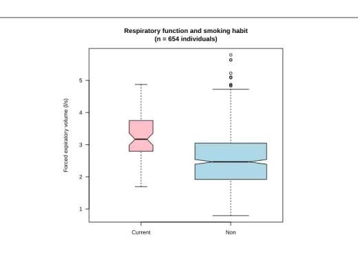
other variables) for 654 human individuals:

• FEV: a quantitavive variable (in l.s−1_{) which name is an acronym for}

“Forced Expiratory Volume”. This is the volume of air expelled after

one second of constant effort, the higher the value is, the better for your health it is.

• Smoker: a binary qualitative variable stating whether the individual is a current smoker of cigarettes (Current) or not (Non).

T

he following code was used to download the data from the internet and

to save it in a local file in XDR [139] format:

path <- "http://www.statsci.org/data/general/fev.txt" fev <- read.table(path, sep = "\t", header = TRUE) save(fev, file = "local/fev.Rda")

W

e want to study the impact of smoking on respiratory performance. Let’s

use the famous Student’s t-test [40]:

load("local/fev.Rda")

t.test(FEV~Smoker, data = fev)

Welch Two Sample t-test data: FEV by Smoker

t = 7.1496, df = 83.273, p-value = 3.074e-10

alternative hypothesis: true difference in means is not equal to 0 95 percent confidence interval:

0.5130126 0.9084253 sample estimates:

mean in group Current mean in group Non

3.276862 2.566143

A

t any decent α critical level, we reject the null hypothesis, there is as

ex-pected an effect of smoking on respiratory performances. Figure 2.2 page 8 illustrate this in a different way: since the notches of the two boxplots do not overlap then, at a critical level of 5%, we can reject the null hypothesis stat-ing that the medians of the respiratory function are the same between the two groups. But, wait a minute, the results are better in the smoking group! Smok-ing is of course not good for your health, so why the smokSmok-ing group has better respiratory results? Exteremly wrong conclusions are at hand when a nuisance parameter is neglected, as it is the case here.

(16)

Current Non 1 2 3 4 5

Respiratory function and smoking habit (n = 654 individuals) F orced e xpir ator y v olume (l/s)

Figure 2.2: Influence of smoking on respiratory function with smokers in

pink and non-smokers in blue. The code for this figure is given p. ??.

S

poiler alert! I don’t want to ruin you the pleasure of discovering by yourself

what is the nuisance parameter here. All the necesary information is present in the variables available in the dataset to figure out what’s going on here. Just

play with the data, so easy with , before reading the following in a mirror.

Asi mple su mm ar y( fe v) will give you anh in tb ys how ing that th ere is av ariab le Ag er angin gfr om3 to 19y ears, our in div idu als are inf actc hil dren s. Theage is an uisan cep aramet erb ecau seit hasa stron ge ffect ont he for ced expi rat ory vol ume ase vide nced by wi th (f ev , pl ot (A ge , FE V) ). All ch ild ren that are less th an9 year sol dar enon smok ers, so th att hen on-smok in ggr oupi sen riche db y ind iv idu alswi th lo wf ev val ues, yiel din gt oth es puriou sr esul twhe nage is not tak eni nto accoun t.

L

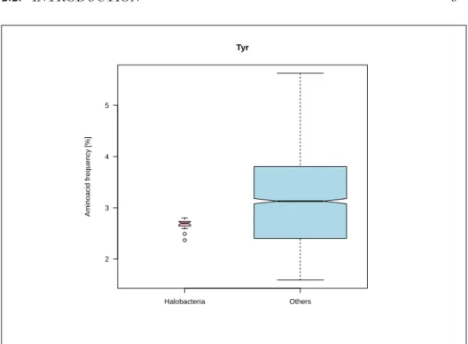
et’s give now a simple example of GC content as a nuisance parameter.

Sup-pose that you are interested in the tyrosine content in Halobacteria because this class is known to have a special proteome content. Figure 2.3 page 9 shows that there is an extremly significant depletion of tyrosine in Halobacteria. This is completely wrong since they are in the opposite enriched in this aminoacid as we will see in section 2.3.4 page 25 where the GC content is taken into account. That’s why Sueoka’s plot is so important.

2.2.4 Aminoacid frequencies under neutral conditions

T

he function giving aminoacid frequencies as function of GC content, θ, in

(17)

Halobacteria Others 2 3 4 5 Tyr Aminoacid frequency [%]

Figure 2.3: Halobacteria are apparently depleted in tyrosine when the GC

content is not taken into account. The code for this figure is given p. ??.

P (θ, aa) = f (θ)

8 − (1 − θ)2_{(1 + θ)} (2.7)

where f (θ) is different from aminoacid to aminoacid:

f (θ) =                                (1 − θ)2(2 − θ) if aa ∈ {Ile}

(1 − θ)2 if aa ∈ {Phe, Lys, Tyr, Asn}

1 − θ2 _{if aa ∈ {Leu}}

(1 − θ)2_θ _{if aa ∈ {Met}}

(1 − θ)θ if aa ∈ {Asp, Glu, His, Gln, Cys}

2(1 − θ)θ if aa ∈ {Val, Thr}

3(1 − θ)θ if aa ∈ {Ser}

(1 − θ)θ2 _{if aa ∈ {Trp}}

θ(θ + 1) if aa ∈ {Arg}

2θ2 _{if aa ∈ {Gly, Pro, Ala}}

(2.8)

The corresponding code is:

aatheo <- function(the, aa){ den <- 8 - (1 - the)^2*(1 + the)

if(aa %in% c("Ile")) return(((2 - the)*(1 - the)^2)/den)

if(aa %in% c("Phe", "Lys", "Tyr", "Asn")) return((1 - the)^2/den) if(aa %in% c("Leu")) return((1 - the^2)/den)

if(aa %in% c("Met")) return((the*(1 - the)^2)/den)

if(aa %in% c("Asp", "Glu", "His", "Gln", "Cys")) return((the*(1 - the))/den) if(aa %in% c("Val", "Thr")) return((2*the*(1 - the))/den)

(18)

if(aa %in% c("Trp")) return(((1 - the)*the^2)/den) if(aa %in% c("Arg")) return(((1 + the)*the)/den) if(aa %in% c("Gly", "Pro", "Ala")) return((2*the^2)/den) stop("unknown aa")

}

This model defines three classes of aminoacids:

classaa <- function(aa){

if(nchar(aa) == 1) aa <- aaa(aa) # 6 aa decreasing with GC content:

if(aa %in% c("Ile", "Phe", "Lys", "Tyr", "Asn", "Leu")) return(1) # 4 aa increasing with GC content:

if(aa %in% c("Gly", "Pro", "Ala", "Arg")) return(3) # 10 aa poorly affected by GC content:

return(2) }

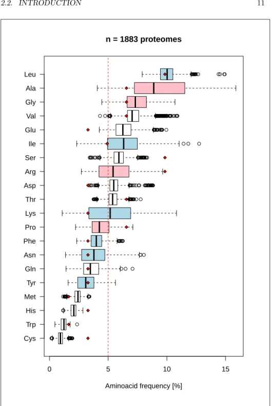
F

igure 2.4 page 11 shows the distribution of aminoacid is far from uniform

and poorly explained by the number of codons per aminoacid. There are clearly selective constraints here. Here is an utility function to explore aminoacid frequencies:

showaa <- function(aalist){ x <- tdd$tdgc

y <- rowSums(cbind(tdd[ , which(colnames(tdd) %in% aalist)], 0)) plot(x, y, xlim = c(0, 100), ylim = c(0, max(y)), las = 1,

xlab = "GC content [%]", ylab = "Aminoacid content [%]",

pch = 19, cex = tdd$cex, main = paste(aalist, collapse = " "), col = col2alpha("black", 0.25)) isa <- which(tdd$superkingdom == 2157)

points(x[isa], y[isa], pch = 21, bg = col2alpha("red", 0.8), cex = tdd$cex[isa]) ish <- which(tdd$class == 183963) # Halobacteria

points(x[ish], y[ish], pch = 21, bg = col2alpha("orange", 0.8), cex = tdd$cex[ish]) ishq <- which(tdd$genus == 293431)

points(x[ishq], y[ishq], pch = 21, bg = col2alpha("yellow", 0.8), cex = tdd$cex[ishq]) abline(lm(y~x), lty = 2)

xx <- seq(0, 100, le = 256) aath <- rep(0, 256)

for(aa in aalist) aath <- aath + sapply(xx/100, function(x) 100*aatheo(x, aa))

lines(xx, aath, type = "l")

legend("bottomleft", inset = 0.02, legend = c("Archaea - not Halobacteria", "Halobacteria - not Haloquadratum spp.",

"Haloquadratum spp.", "Eubacteria"), pch = 21,

pt.bg = c(col2alpha("red", 0.8), col2alpha("orange", 0.8), col2alpha("yellow", 0.8), col2alpha("black", 0.25)), bg = grey(0.9))

mtext(bquote(r^2 == .(signif(cor(x,y)^2, 3))), adj = 0) mtext(bquote(alpha == .(signif(lm(y~x)$coef[2], 3))), adj = 1) legend <- c("Linear fit", "Neutral model")

legend("bottomright", inset = 0.02, bg = grey(0.9), lty = c(2, 1), legend = legend) }

This code is used to generate all figures:

todo <- aaa()[-1] for(i in todo){

fname <- paste("figs/auto-", i, ".pdf", sep = "") pdf(fname)

showaa(i) dev.off() }

2.2.5 Aminoacid classes with respect to GC content

T

he model 2.8 defines three classes of aminoacids with respect to their

(19)

Cys Trp His Met Tyr Gln Asn Phe Pro Lys Thr Asp Arg Ser Ile Glu Val Gly Ala Leu 0 5 10 15 n = 1883 proteomes Aminoacid frequency [%]

Figure 2.4: Distribution of aminoacid frequencies in the dataset. The

verti-cal red line is what would be expected for a uniform distribution, that is 1

20

for all aminoacids. The red diamond points are the expected distribution

for a uniform codon usage, that is 1

61 for each coding codon. Aminoacids of

class 1 are in blue, and class 3 in red. The variance is higher for those two

last classes both affected by the GC content. The code for this figure is

(20)

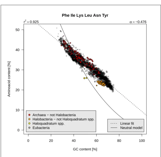
0 20 40 60 80 100 0 10 20 30 40 50

Phe Ile Lys Leu Asn Tyr

GC content [%]

Aminoacid content [%]

Archaea − not Halobacteria

Halobacteria − not Haloquadratum spp. Haloquadratum spp.

Eubacteria

r2=0.925 α =−0.476

Linear fit Neutral model

Figure 2.5: Class 1 aminoacids frequencies as function of GC content. The code for this figure is given p. ??.

(21)

1. Six aminoacids whose frequencies are expected to decrease with GC con-tent. Figure 2.5 page 12 shows that they represent about 45% of aminoacids in low-GC bacteria and about 20% in high-GC bacteria. On average, an increase of 10% for the GC content will decrease their frequency by 5%. 2. Ten aminoacids whose frequencies are poorly affected by GC content.

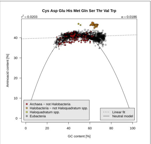
Fig-ure 2.6 page 14 shows that they represent about 40% of aminoacids, that is slighly less than the 50% we would expect from a uniform distribution. 3. Four aminoacids whose frequencies are expected to increase with GC

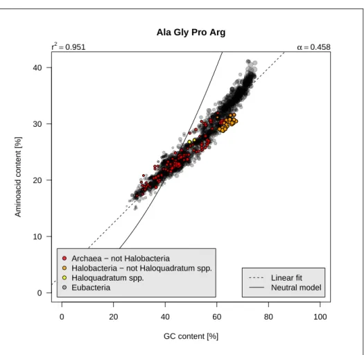
content. Figure 2.7 page 15 shows that they represent about 15% of

aminoacids in low-GC bacteria and about 40% in high-GC bacteria. On average, an increase of 10% for the GC content will increase their frequency by 5%.

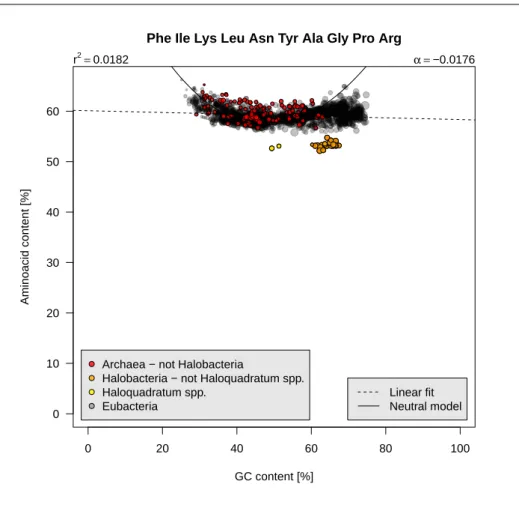
F

igure 2.8 page 16 shows that the decrease in class 1 is compensated by the

increase in class 3 (this is logical since class 2 is almost constant and the grand total 100% by construction) so that these 10 aminoacids represent about 60% of aminoacids, that is slighly more than the 50% we would expect from a uniform distribution.

(22)

0 20 40 60 80 100 0 10 20 30 40

Cys Asp Glu His Met Gln Ser Thr Val Trp

GC content [%]

Eubacteria

r2=0.0203 α =0.0186

(23)

0 20 40 60 80 100 0 10 20 30 40

Ala Gly Pro Arg

GC content [%]

Eubacteria

r2=0.951 α =0.458

(24)

0 20 40 60 80 100 0 10 20 30 40 50 60

Phe Ile Lys Leu Asn Tyr Ala Gly Pro Arg

GC content [%]

Eubacteria

r2=0.0182 α =−0.0176

Figure 2.8: Class 1 and class 3 aminoacids frequencies as function of GC

(25)

2.3 Class 1 aminoacids

2.3.1 Isoleucine

I

soleucine is a non-polar uncharged aliphatic aminoacid encoded by three

codons. It is highly sensitive to the GC content since its frequency decreases from 12% in low-GC bacteria to 2% in high-GC bacteria, that is a factor 6. Figure 2.9 page 18 shows that the results are consistent with [136]. The linear

model summarises well the general trend (r2 _{≈ 0.9) but the distribution of}

residual is non-random, with a sigmoidal shape. There is a small trend for low-GC archaea to use more Ile than eubacteria. There is also a small trend for halobacteria to use less Ile than eubacteria. Its frequency is close to what would be expected from uniform codon usage at GC below 50% but higher at GC above 50% as if there were a selective pressure to maintain a minimal frequency. The two top outliers are:

tdd[tdd$Ile > 11.5, "organism"]

[1] "buchnera_aphidicola" "wigglesworthia_glossinidia"

T

he two outliers, Buchnera aphidicola [87] and Wigglesworthia glossinidia [1],

are both low-GC small genomes endosymbiont bacteria. Their Ile frequency

is above 11.5%.The two following outliers are: Could this be a

con-sequence of the dereg-ulation of aminoacid biosynthetic pathways? Could this be a con-sequence of the dereg-ulation of aminoacid biosynthetic pathways?

tdd[tdd$Ile < 11.5 & tdd$Ile > 11, "organism"]

[1] "ignisphaera_aggregans" "picrophilus_torridus"

T

he two following outliers, Picrophilus torridus [124] and Ignisphaera

aggre-gans [91], are both acidophilic (pH 0.7 and 6.4 respectively) archaeae with

high Topt (60°C and 92°C, respectively).

0 20 40 60 80 100 0 2 4 6 8 10 12 Ile GC content [%] Aminoacid content [%]

Archaea − not Halobacteria Halobacteria − not Haloquadratum spp. Haloquadratum spp.

Eubacteria

r2₌_0.897 _{α =}_−0.135

(26)

20 30 40 50 60 70 80 0 2 4 6 8 10 Ile (unstable) Genomic GC content [%] Aminoacid frequency [%] r2=0.68 α =−0.098

Figure 2.9: Re-creation of Sueoka’s plot with data from table 1 in [136]. The number of point supperpositions, if any, is indicated by the number of vertices in the stars. The line is the best quadratic fit without including Tetrahymena pyriformis denoted by the black point. Slope in [136] was

α = −0.098. The code for this figure is given p. ??.

2.3.2 Phenylalanine

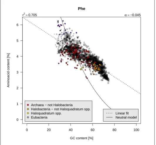
P

henylalanine is an aromatic neutral nonpolar aminoacid encoded by two

codons. It is sensitive to the GC content since its frequency decreases from 6% in low-GC bacteria to 2% in high-GC bacteria, that is a factor 3. Figure 2.10 page 20 shows that the results are consistent with [136]. The linear model

summarises well the general trend (r2_{≈ 0.7) but the distribution of residual is}

non-random, with a sigmoidal shape. Its frequency is close to what would be expected from uniform codon usage at GC below 40% but higher at GC above 40% as if there were a selective pressure to maintain a minimal frequency. Most low-Phe are archaeae but not all archaeae are low-Phe. The top-outlier are from two genera (Borrelia = Borreliella and Campylobacter ):

tdd[tdd$Phe > 5.8, "organism"] [1] "borrelia_afzelii" "borrelia_burgdorferi" [3] "borrelia_garinii" "borreliella_bavariensis" [5] "borreliella_spielmanii" "campylobacter_coli" [7] "campylobacter_hominis" "campylobacter_insulaenigrae" [9] "campylobacter_jejuni" "campylobacter_lari" [11] "campylobacter_upsaliensis" "campylobacter_ureolyticus" [13] "campylobacter_volucris"

(27)

0 20 40 60 80 100 0 1 2 3 4 5 6 Phe GC content [%] Aminoacid content [%]

Eubacteria

r2=0.705 α =−0.045

F

igure 2.11 page 21 shows that the species from these two genera are generally

rich in Phe, however the observed frequencies are not anomalously high as compared to what is expected from a uniform codon usage. This is somewhat redundant to say that they have a GC-poor genome.

(28)

20 30 40 50 60 70 80 0 1 2 3 4 5 6 Phe (stable) Genomic GC content [%] Aminoacid frequency [%] r2=0.44 α =−0.04

(29)

0 20 40 60 80 100 0 1 2 3 4 5 6 Phe GC content [%] Aminoacid content [%]

Eubacteria

r2=0.705 α =−0.045

Figure 2.11: Phenylalanine as function of GC content with species from

Borreliella or Campylobacter genera in purple. The code for this figure

(30)

2.3.3 Lysine

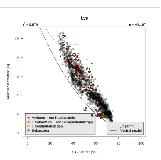
L

ysine is a basic charged aliphatic amino acid encoded by two codons. It is

highly sensitive to the GC content since its frequency decreases from 10% in low-GC bacteria to 1% in high-GC bacteria, that is a factor 10. Figure 2.13 page 24 shows that the results are consistent with [136]. The linear model

summarises well the general trend (r2 _{≈ 0.9). Its frequency is close to what}

would be expected from uniform codon usage, but always higher as if there were a selective pressure to increase its frequency. Halobacteria tend to avoid this aminoacid, a known phenomenon [56]. The species with less Lys than predicted by the neutral model are:

tdd[100*sapply(tdd$tdgc/100, aatheo, aa = "Lys") > tdd$Lys, "organism"]

[1] "chloroflexus_aggregans" "chloroflexus_aurantiacus" [3] "haloquadratum_sp" "haloquadratum_walsbyi" [5] "halorubrum_sp" "herpetosiphon_aurantiacus" [7] "natrialba_magadii" "roseiflexus_castenholzii" [9] "thermomicrobium_roseum"

F

rom those species, halobacteria are Haloquadratum walsbyi, Halorubrum sp.

and Natrialba magadii. Remaining species are all Chloroflexi (Chlorobac-teria) and figure 2.12 page 23 shows that there is a trend for species from this group to be depleted in Lys.

0 20 40 60 80 100 0 2 4 6 8 10 Lys GC content [%] Aminoacid content [%]

Eubacteria

r2₌_0.874 _{α =}_−0.167

(31)

0 20 40 60 80 100 0 2 4 6 8 10 Lys GC content [%] Aminoacid content [%]

Eubacteria

r2=0.874 α =−0.167

Figure 2.12: Lysine as function of GC content with species from Chloroflexi

(32)

20 30 40 50 60 70 80 0 2 4 6 8 10 12 Lys (stable) Genomic GC content [%] Aminoacid frequency [%] r2=0.44 α =−0.084

(33)

2.3.4 Tyrosine

T

yrosine is an aromatic polar hydrophobic aminoacid encoded by two codons.

It is sensitive to the GC content since its frequency decreases from 5.5% in low-GC bacteria to 1.5% in high-GC bacteria, that is a factor 3.5. Figure 2.14 page 26 shows that the results are consistent with [136]. The linear model

sum-marises well the general trend (r2_{≈ 0.7). Its frequency is close to what would be}

expected from uniform codon usage, but lower at GC below 50% and higher at GC above 50% as if there were a selective pressure to avoid too extreme values. Halobacteria tend to favor Tyr but there are two exceptions: Haloquadratum walsbyi [21] and Halorubrum sp.

0 20 40 60 80 100 0 1 2 3 4 5 Tyr GC content [%] Aminoacid content [%]

Archaea − not Halobacteria Halobacteria − not Haloquadratum spp. Haloquadratum spp. Eubacteria r2=0.719 α =−0.0536 Linear fit Neutral model

2.3.5 Asparagine

A

sparagine is a polar aliphatic aminoacid encoded by two codons. It is very

sensitive to the GC content since its frequency decreases from 8% in low-GC bacteria to 1% in high-low-GC bacteria, that is a factor 8. The linear model

summarises well the general trend (r2 _{≈ 0.9). Its frequency is close to what}

would be expected from uniform codon usage, but higher at GC above 50% as if there were a selective pressure to avoid a too low value. Halobacteria tend to avoid lightly Asn.

(34)

20 30 40 50 60 70 80 0 1 2 3 4 5 Tyr (stable) Genomic GC content [%] Aminoacid frequency [%] r2=0.41 α =−0.046

α = −0.047. The code for this figure is given p. ??.

0 20 40 60 80 100 0 2 4 6 8 Asn GC content [%] Aminoacid content [%]

Eubacteria

r2=0.876 α =−0.0986

(35)

2.3.6 Leucine

L

eucine is a non-polar aliphatic aminoacid encoded by 6 codons. It is

sup-posed to decrease with GC but increase a little from 9.5% in low-GC bacte-ria to 10.5% in high-GC bactebacte-ria, that is a factor 1.1. Figure 2.16 page 29 shows that the results are consistent with [136]. The linear model summarises poorly

the general trend (r2_{≈ 0.14). Halobacteria tend to avoid this aminoacid. The}

top-outliers are:

tdd[which(tdd[ ,"Leu"] > 14), c("organism", "domain", "topt", "Leu")]

organism domain topt Leu 2175 thermus_oshimai Bacteria 65 14.92963 2176 thermus_scotoductus Bacteria 66 14.40196 2177 thermus_sp Bacteria 67 14.88733 2178 thermus_thermophilus Bacteria 75 14.52119

T

he four outliers are all thermophilic eubacteria from the Thermus genus (viz.

T. oshimai [154] T. scotoductus [63], T. thermophilus [97, 155], T. sp. [17]) and figure 2.15 page 28 shows that all species from this genus have a high Leu content. This is interesting because if this high-Leu frequency is an adaptation for high temperature, then there is no universal response for thermophily on aminoacid content. 0 20 40 60 80 100 0 5 10 15 Leu GC content [%] Aminoacid content [%]

Eubacteria

r2=0.13 α =0.0232

(36)

0 20 40 60 80 100 0 5 10 15 Leu GC content [%] Aminoacid content [%]

Eubacteria

r2=0.13 α =0.0232

Figure 2.15: Leucine as function of GC content with species from Thermus

(37)

20 30 40 50 60 70 80 0 2 4 6 8 10 12 Leu (stable) Genomic GC content [%] Aminoacid frequency [%] r2=0.02 α =−0.0062

(38)

Bibliography of the Thermus genus Bibliography of the Thermus genus

2.4 Class 2 aminoacids

2.4.1 Methionine

M

ethionine is nonpolar aliphatic aminoacid encoded by a single codon. It

is poorly sensitive to the GC content with frequency ranging from 1.5% to 3.5%, always above about 1% of what would be expected from uniform codon usage. It’s only for GC greater than 50% that a decrease is observed. The linear

model summarises poorly the general trend (r2 _{≈ 0.2). Figure 2.17 page 31}

shows that the results are consistent with [136]. Halobacteria tend to avoid Met. 0 20 40 60 80 100 0.0 0.5 1.0 1.5 2.0 2.5 3.0 3.5 Met GC content [%] Aminoacid content [%]

Eubacteria

r2₌_0.169 _{α =}_−0.0123

(39)

20 30 40 50 60 70 80 0 1 2 3 4 5 6 Met (unstable) Genomic GC content [%] Aminoacid frequency [%] r2=0.062 α =−0.031

α = −0.024, different from here. I was unable to find the reason for this

(40)

2.4.2 Aspartic acid

A

spartic acid is an acidic aminoacid encoded by two codons. It is almost

unaffected by the GC content with an average concentration of 5.1% in low-GC bacteria to 5.9% in high-low-GC bacteria, that is a factor 1.15. The linear model

summarises poorly the general trend (r2 _{≈ 0.1). Its frequency is above about}

2% of what would be expected from uniform codon usage. Halobacteria are highly enriched in Asp with a frequency close to 8%, a known phenomena [56]. The bottom outliers are:

tdd[tdd$Asp < 3.7, "organism"]

[1] "thermus_oshimai" "thermus_scotoductus" "thermus_sp" [4] "thermus_thermophilus"

T

he four outliers are all thermophilic eubacteria from the Thermus genus (viz.

T. oshimai [154] T. scotoductus [63], T. thermophilus [97, 155], T. sp. [17]) and figure 2.18 page 33 shows that all species from this genus have a low Asp content. This is interesting because if this low-Asp frequency is an adaptation for high temperature, then there is no universal response for thermophily on aminoacid content. 0 20 40 60 80 100 0 2 4 6 8 Asp GC content [%] Aminoacid content [%]

Eubacteria

r2₌_0.0864 _{α =}_0.0144

(41)

0 20 40 60 80 100 0 2 4 6 8 Asp GC content [%] Aminoacid content [%]

Eubacteria

r2=0.0864 α =0.0144

Figure 2.18: Aspartic acid as function of GC content with species from

(42)

2.4.3 Glutamic acid

G

lutamic acid is an acidic aminoacid encoded by two codons. It is almost

unaffected by the GC content with an average concentration of 7.2% in low-GC bacteria to 5.5% in high-low-GC bacteria, that is a factor 1.3. The linear model

summarises poorly the general trend (r2 _{≈ 0.2). Its frequency is above about}

3-5% of what would be expected from uniform codon usage. Halobacteria are highly enriched in Glu with a frequency close to 9%, a known phenomena [56]. The bottom outliers are:

tdd[tdd$Glu < 4.3, "organism"]

[1] "lactobacillus_shenzhenensis" "mycobacterium_leprae"

T

he two outliers are Lactobacillus shenzhenensis and Mycobacterium leprae

but figure 2.19 page 35 shows that this is not a general trend for species from these genera.

0 20 40 60 80 100 0 2 4 6 8 10 Glu GC content [%] Aminoacid content [%]

Eubacteria

r2=0.209 α =−0.0352

(43)

0 20 40 60 80 100 0 2 4 6 8 10 Glu GC content [%] Aminoacid content [%]

Eubacteria

r2=0.209 α =−0.0352

Figure 2.19: Glutamic acid as function of GC content with species from

Lactobacillus and Mycobacterium genera in purple. The code for this

(44)

2.4.4 Serine

S

erine is a polar aminoacid encoded by 6 codons. Its frequency ranges on

average from 6.7% in low-GC bacteria to 5.2% in high-GC bacteria, that is a factor 1.3. Figure 2.21 page 38 shows that the results are consistent with [136].

The linear model summarises poorly the general trend (r2_{≈ 0.3). The bottom}

outliers are: tdd[tdd$Ser < 4.2, "organism"] [1] "marinithermus_hydrothermalis" "oceanithermus_profundus" [3] "rhodothermus_marinus" "thermaerobacter_marianensis" [5] "thermaerobacter_subterraneus" "thermus_oshimai" [7] "thermus_scotoductus" "thermus_sp" [9] "thermus_thermophilus"

T

hese are all thermophilic species but figure 2.20 page 37 show that a low-Ser

is not a property shared by all thermophilic species.

0 20 40 60 80 100 0 2 4 6 8 Ser GC content [%] Aminoacid content [%]

Eubacteria

r2₌_0.34 _{α =}_−0.03

(45)

0 20 40 60 80 100 0 2 4 6 8 Ser GC content [%] Aminoacid content [%]

Eubacteria

r2=0.34 α =−0.03

Figure 2.20: Serine acid as function of GC with colors for thermophilic

(46)

20 30 40 50 60 70 80 0 2 4 6 8 Ser (unstable) Genomic GC content [%] Aminoacid frequency [%] r2=0.054 α =−0.017

(47)

2.4.5 Valine

V

aline is a non-polar aliphatic aminoacid encoded by 4 codons. Its frequency

ranges on average from 6% in low-GC bacteria to 8.5% in high-GC bacteria, that is a factor 1.4. The linear model summarises poorly the general trend

(r2_{≈ 0.5). Figure 2.24 page 42 shows that this trend was not visible in [136].}

Halobacteria tend to favour this aminoacid. There seems to be a cluster of points at high-GC as exemplified by figure 2.22 page 40 and figure 2.23 page 41 shows that it corresponds more or less to the actinobacteria class (high-GC gram+ bacteria TID = 1760). 0 20 40 60 80 100 0 2 4 6 8 10 Val GC content [%] Aminoacid content [%]

Eubacteria

r2=0.495 α =0.0505

(48)

Val GC content [%] Aminoacid frequency [%] 30 40 50 60 70 5 6 7 8 9 10 11

Figure 2.22: Density plot of valine as function of GC. Note the cluster at

(49)

0 20 40 60 80 100 0 2 4 6 8 10 Val GC content [%] Aminoacid content [%]

Eubacteria

r2=0.495 α =0.0505

Figure 2.23: Valine as function of GC with actinobacteria in purple. The code for this figure is given p. ??.

(50)

20 30 40 50 60 70 80 0 2 4 6 8 10 12 Val (stable) Genomic GC content [%] Aminoacid frequency [%] r2=0.026 α =0.0076

(51)

Check bottom outliers Check bottom outliers

2.4.6 Threonine

T

hreonine is a polar, uncharged aminoacid enocoded by 4 codons. Its

fre-quency is close to 5% and poorly affected by the GC-content. Figure 2.25 page 44 shows that the results are consistent with [136]. Haloquadratum walsbyi is an outlier with a Thr content of 7.8%. As for Val there seems to be a cluster of points at high-GC as exemplified by figure 2.26 page 45 and figure 2.27 page 46 shows that it corresponds more or less to the actinobacteria class (high-GC gram+ bacteria TID = 1760).

0 20 40 60 80 100 0 2 4 6 8 Thr GC content [%] Aminoacid content [%]

Eubacteria

r2=0.057 α =0.0107

(52)

20 30 40 50 60 70 80 0 2 4 6 8 Thr (unstable) Genomic GC content [%] Aminoacid frequency [%] r2=7.4e−06 α =0.00015

(53)

Val GC content [%] Aminoacid frequency [%] 30 40 50 60 70 4 5 6 7

Figure 2.26: Density plot of threonine as function of GC. Note the cluster

(54)

0 20 40 60 80 100 0 2 4 6 8 Thr GC content [%] Aminoacid content [%]

Eubacteria

r2=0.057 α =0.0107

Figure 2.27: Threonine as function of GC with actinobacteria in purple.

(55)

2.4.7 Histidine

H

istidine is a positively charged aminoacid encoded by 2 codons. Its

fre-quency ranges on average from 1.7% in low-GC bacteria to 2.3% in high-GC bacteria, that is a factor 1.4. Figure 2.28 page 48 shows that the results are consistent with [136]. The linear model summarises poorly the general trend

(r2_{≈ 0.2).} 0 20 40 60 80 100 0.0 0.5 1.0 1.5 2.0 2.5 His GC content [%] Aminoacid content [%]

Eubacteria

r2₌_0.234 _{α =}_0.0121

(56)

20 30 40 50 60 70 80 0 1 2 3 4 His (stable) Genomic GC content [%] Aminoacid frequency [%] r2=0.092 α =−0.01

(57)

2.4.8 Glutamine

G

utamine is a charge-neutral, polar aminoacid encoded by 2 codons. It is

almost unaffected by the GC content with an average frequency of 3.5% close to what would be expected from an uniform codon usage. This aminoacid is clearly avoided in archaea as compared to eubacteria. The top-outliers are:

tdd[tdd$Gln > 6.2, "organism"]

[1] "lactobacillus_mellifer" "lactobacillus_mellis"

T

hey are all from the genus Lactobacillus but figure 2.29 page 50 show that

this is not a general property of the species from this genus.

0 20 40 60 80 100 0 1 2 3 4 5 6 7 Gln GC content [%] Aminoacid content [%]

Eubacteria

r2₌_0.00751 _{α =}_−0.00615

(58)

0 20 40 60 80 100 0 1 2 3 4 5 6 7 Gln GC content [%] Aminoacid content [%]

Eubacteria

r2=0.00751 α =−0.00615

Figure 2.29: Glutamine as function of GC with species from Lactobacillus

(59)

2.4.9 Cysteine

C

ysteine has a thiol side chain and is encoded by 2 codons. It frequency is

poorly affected by the GC content with an average concentration at about 1%, less than what would be expected from a uniform codon usage.

0 20 40 60 80 100 0.0 0.5 1.0 1.5 2.0 Cys GC content [%] Aminoacid content [%]

Archaea − not Halobacteria Halobacteria − not Haloquadratum spp. Haloquadratum spp. Eubacteria r2=0.0116 α =−0.00232 Linear fit Neutral model

2.4.10 Tryptophane

T

ryptophane is non-polar aromatic amino acid encoded by a single codon.

It a rare aminoacid with frequency ranging on average from 0.75% in low-GC bacteria to 1.6% in high-low-GC bacteria, that is a factor 2. There is a trend for halobacteria to avoid this aminoacid. The top outlier is:

tdd[tdd$Trp > 2, c("organism", "Trp", "topt")]

organism Trp topt 2064 sulfobacillus_acidophilus 2.352197 45

S

ince Sulfobacillus acidophilus is the only species available for the Sulfobacillus

(60)

0 20 40 60 80 100 0.0 0.5 1.0 1.5 2.0 Trp GC content [%] Aminoacid content [%]

Archaea − not Halobacteria Halobacteria − not Haloquadratum spp. Haloquadratum spp. Eubacteria r2=0.617 α =0.0168 Linear fit Neutral model

2.5 Class 3 aminoacids

2.5.1 Arginine

A

rginine is a charged, aliphatic aminoacid encoded by 6 codons. It is very

sensitive to the GC content with a frequency ranging on average from 2.6% in low-GC bacteria to 8.3% in high-GC bacteria, that is a factor 3.2. The linear

model is a good summary (r2≈ 0.9). Figure 2.30 page 53 shows that the results

are consistent with [136]. All halobacteria but Haloquadratum walsbyi tend to avoid this amino-acid.

(61)

20 30 40 50 60 70 80 0 2 4 6 8 10 Arg (stable) Genomic GC content [%] Aminoacid frequency [%] r2=0.5 α =0.089

α = 0.089. The code for this figure is given p. ??.

0 20 40 60 80 100 0 2 4 6 8 10 Arg GC content [%] Aminoacid content [%]

Eubacteria

r2₌_0.899 _{α =}_0.117

(62)

2.5.2 Alanine

A

lanine is a nonpolar, aliphatic aminoacid encoded by 4 codons. It is very

sensitive to the GC content with a frequency ranging on average from 4.5% in low-GC bacteria to 14% in high-GC bacteria, that is a factor 3.1. The linear

model is a good summary (r2_{≈ 0.9). Figure 2.31 page 55 shows that the results}

are consistent with [136]. All halobacteria but Haloquadratum walsbyi tend to avoid this amino-acid.

0 20 40 60 80 100 0 5 10 15 Ala GC content [%] Aminoacid content [%]

Eubacteria

r2₌_0.889 _{α =}_0.194

(63)

20 30 40 50 60 70 80 0 5 10 15 20 Ala (stable) Genomic GC content [%] Aminoacid frequency [%] r2=0.67 α =0.16

(64)

2.5.3 Proline

P

roline is a nonpolar, aliphatic aminoacid encoded by 4 codons. It is very

sensitive to the GC content with a frequency ranging on average from 2.5% in low-GC bacteria to 6% in high-GC bacteria, that is a factor 2.4. The linear

model is a good summary (r2_{≈ 0.9). Figure 2.32 page 57 shows that the results}

are consistent with [136]. All halobacteria but Haloquadratum walsbyi tend to avoid this amino-acid. The top outliers are:

tdd[tdd$Pro > 6.6, "organism"] [1] "frankia_alni" "frankia_sp" [3] "isosphaera_pallida" "kitasatospora_setae" [5] "roseomonas_cervicalis" "streptomyces_cattleya" [7] "thermaerobacter_marianensis" "thermaerobacter_subterraneus" 0 20 40 60 80 100 0 1 2 3 4 5 6 7 Pro GC content [%] Aminoacid content [%]

Eubacteria

r2=0.855 α =0.0701

(65)

20 30 40 50 60 70 80 0 1 2 3 4 5 6 7 Pro (stable) Genomic GC content [%] Aminoacid frequency [%] r2=0.26 α =0.024

(66)

2.5.4 Glycine

G

lycine has a single hydrogen atom as its side chain and is encoded by 4

codons. It is very sensitive to the GC content with a frequency ranging on average from 5.5% in low-GC bacteria to 9.5% in high-GC bacteria, that is a

factor 1.7. The linear model is a good summary (r2_{≈ 0.9). Figure 2.33 page 59}

shows that the results are consistent with [136]. Top outliers are:

tdd[tdd$Gly > 10, "organism"] [1] "mycobacterium_marinum" "rubrobacter_xylanophilus" [3] "thermaerobacter_marianensis" "thermaerobacter_subterraneus" 0 20 40 60 80 100 0 2 4 6 8 10 Gly GC content [%] Aminoacid content [%]

Eubacteria

r2=0.884 α =0.0779

(67)

20 30 40 50 60 70 80 0 5 10 15 Gly (unstable) Genomic GC content [%] Aminoacid frequency [%] r2=0.28 α =0.051

(68)

2.6 Evolution of hydrolysis sensitive aminoacids

with GC content

2.6.1 Aspartic acid and asparagine

showaa(c("Asp", "Asn")) 0 20 40 60 80 100 0 2 4 6 8 10 12 14 Asp Asn GC content [%] Aminoacid content [%]

Eubacteria

r2=0.623 α =−0.0841

F

igure 2.34 page 61 shows that the results here are consistent with those

(69)

20 30 40 50 60 70 80 0 5 10 15 AspX (stable) Genomic GC content [%] Aminoacid frequency [%] r2=0.2 α =−0.054

(70)

2.6.2 Glutamic acid and glutamine

showaa(c("Glu", "Gln")) 0 20 40 60 80 100 0 2 4 6 8 10 12 Glu Gln GC content [%] Aminoacid content [%]

Eubacteria

r2=0.274 α =−0.0413

F

igure 2.35 page 63 shows that the results here are consistent with those

(71)

20 30 40 50 60 70 80 0 5 10 15 GluX (stable) Genomic GC content [%] Aminoacid frequency [%] r2=0.15 α =−0.043

α = −0.052 is different from here. I was unable to find the reason for this

(72)

2.7 Evolution of charged aminoacids with GC

content

2.7.1 Negatively charged aminoacid

T

he frequency of negatively charged aminoacids decreases with GC content

from 18% in low-GC bacteria to 14% in high-GC bacteria, that is a factor 1.3.

showaa(c("Asp", "Glu", "Tyr", "Cys"))

0 20 40 60 80 100 0 5 10 15 20

Asp Glu Tyr Cys

GC content [%]

Eubacteria

r2=0.362 α =−0.0767

2.7.2 Positively charged aminoacid

T

he frequency of positively charged aminoacids also decreases with GC

con-tent from 13.8% in low-GC bacteria to 11.8% in high-GC bacteria, that is a factor 1.2. Note that the frequency of positively charged aminoacids is on the opposite expected to increase with GC content, we have perhaps here a selective pressure on the global charge of the proteins.

(73)

0 20 40 60 80 100 0

5 10 15

Arg Lys His

GC content [%]

Halobacteria − not Haloquadratum spp. Haloquadratum spp. Eubacteria r2=0.28 α =−0.0382 Linear fit Neutral model

2.7.3 Evolution of pI with GC

A

s we may have expected from the simultaneous decrease of positively and

negatively charged aminoacids decribed in the two previous sections, fig-ure 2.36 page 66 shows that pI is unaffected by the GC content.

(74)

0 20 40 60 80 5 6 7 8 9 n = 1883 proteomes GC content [%] pI

Archaea − not Halobacteria Halobacteria − not Haloquadratum Haloquadratum walsbyi Eubacteria

Figure 2.36: Stability of the isoelectric point of proteomes with respect to

(75)

2.8 Summary of outstanding bacterial groups

I

t long has been recognized that proteins from “extreme halophiles” are acidic,

see for instance the 1974 review [66].

Summarize here what was gained from uni-variate anlysis of aminoacid usage in bac-teria

(76)

(77)

Chapter 3

Multivariate analysis of

aminoacid usage

3.1 Loading the dataset

3.2 Utilities

3.2.1 First factorial map orientation

Automate axis orien-tation so as to have al-ways low-GC on the left and thermophilic on the top

3.3 Sanity check

I

n this section I want to check that the results are the same when computing

correspondance analysis of aminoacid usage in two different ways.

3.3.1 Direct CA on aminoacid frequencies

codons <- colnames(tdd[ , 2:65])

facaa <- factor(sapply(codons, function(x) aaa(translate(s2c(x))))) tdaa <- t(apply(tdd[ , 2:65], 1, function(x) tapply(x, facaa, sum))) library(ade4)

checkcoa1 <- dudi.coa(tdaa, scannf = FALSE, nf = 2) swap <- function(dudi, nf){

dudi$li[ , nf] <- -1*dudi$li[ , nf] dudi$co[ , nf] <- -1*dudi$co[ , nf] return(dudi)

}

checkcoa1 <- swap(checkcoa1, 1) # High GC on right checkcoa1 <- swap(checkcoa1, 2) # Thermophiles on top checkplot <- function(dudi){

main <- paste("Aminoacid usage in", nrow(dudi$tab), "bacteria")

plot(dudi$li[ ,1], dudi$li[ ,2], pch = 21, bg = tdd$athermocol, asp = 1, cex = tdd$cex, xlab = "", ylab = "", main = main)

title(xlab = paste("F1 :", signif(100*dudi$eig[1]/sum(dudi$eig), 3), "%")) title(ylab = paste("F2 :", signif(100*dudi$eig[2]/sum(dudi$eig), 3), "%"))

(78)

legend("bottomleft", inset = 0.02,

legend = c("Topt <= 20", "Topt < 59", "Topt >= 59", "Topt > 80"), pch = 21, pt.bg = unique(tdd$athermocols)) } checkplot(checkcoa1) −0.4 −0.2 0.0 0.2 0.4 −0.4 −0.2 0.0 0.2 0.4

Aminoacid usage in 1883 bacteria

F1 : 79.6 % F2 : 6.95 % Topt <= 20 Topt < 59 Topt >= 59 Topt > 80

3.3.2 BCA on codon frequencies

library(seqinr) tdco <- tdd[ , 2:65] codons <- colnames(tdco)

facaa <- factor(sapply(codons, function(x) aaa(translate(s2c(x))))) coa <- dudi.coa(tdco, scannf = F, nf = 2)

checkcoa2 <- t(bca(t(coa), facaa, scannf = FALSE, nf = 2)) checkcoa2 <- swap(checkcoa2, 2) # Thermophiles on top checkplot(checkcoa2)

(79)

−0.4 −0.2 0.0 0.2 0.4 −0.4 −0.2 0.0 0.2 0.4

Aminoacid usage in 1883 bacteria

F1 : 79.6 % F2 : 6.95 % Topt <= 20 Topt < 59 Topt >= 59 Topt > 80

3.3.3 Comparisons

all.equal(checkcoa1$eig, checkcoa2$eig) [1] TRUE all.equal(checkcoa1$li[ , 1], checkcoa2$li[ , 1])

[1] "Mean relative difference: 2"

all.equal(checkcoa1$li[ , 2], checkcoa2$li[ , 2])

[1] TRUE

3.3.4 Conclusion

A

s expected, the results are exactly the same. This is because CA on aminoacid

fequencies is the same analysis as the between group analysis for CA on codon frequencies.

(80)

(81)

Chapter 4

Univariate analysis of

synonymous codon usage

4.1 Utilities definition

4.1.1 Loading the dataset

4.1.2 Computing codon relative frequencies

library(seqinr)

codons <- colnames(tdd[ , 2:65])

facaa <- factor(sapply(codons, function(x) aaa(translate(s2c(x))))) tdc <- t(apply(tdd[ , 2:65], 1, function(x)

unlist(tapply(x, facaa, function(y) 100*y/sum(y))))) tdc <- as.data.frame(tdc)

substr(names(tdc), 4,4) <- "-" # remove the dot for file names tdc$tdgc <- tdd$tdgc

4.1.3 Ploting data

plotcod <- function(codlist){ x <- tdc$tdgc

y <- rowSums(cbind(tdc[ , which(colnames(tdc) %in% codlist)], 0)) plot(x, y, xlim = c(0, 100), ylim = c(0, 100), las = 1,

xlab = "GC content [%]", ylab = "Codon relative frequency [%]",

pch = 19, cex = tdd$cex, main = paste(codlist, collapse = " "), col = col2alpha("black", 0.25)) abline(lm(y~x), lty = 2)

abline(v = 50, lty = 2) abline(h = mean(y), lty = 2) axis(4)

mtext(bquote(r^2 == .(signif(cor(x,y)^2, 3))), adj = 0.5) mtext(paste("Slope =", signif(lm(y~x)$coef[2], 3)), adj = 0) mtext(paste("Intercept =", signif(lm(y~x)$coef[1], 3)), adj = 1) isa <- which(tdd$domain == "Archaea")

points(x[isa], y[isa], pch = 21, bg = col2alpha("red", 0.8), cex = tdd$cex[isa]) ish <- which(tdd$class == 183963) # Halobacteria

points(x[ish], y[ish], pch = 21, bg = col2alpha("orange", 0.8), cex = tdd$cex[ish]) lines(lowess(x, y), col = "red")

ou <- ifelse(lm(y~x)$coef[2] > 0, "toplef", "topright")

(82)

legend(ou, inset = 0.02, legend = c("Archaea - not Halobacteria", "Halobacteria", "Eubacteria"), pch = 21, pt.bg = c(col2alpha("red", 0.8), col2alpha("orange", 0.8), col2alpha("black", 0.25)), bg = grey(0.9)) }

4.1.4 Generation of all figures

This code is used to generate all figures:

todo <- names(tdc)[-65] for(i in todo){

fname <- paste("figs/auto-", i, ".pdf", sep = "") pdf(fname) par(mar = c(5, 4, 4, 0) + 0.1) plotcod(i) dev.off() }

4.2 Introduction

B

ecause there are 64 codons, we need some guideline to structure this

Codon and aminoacid usage in bacteria (Haeckel, 1874)

(Haeckel, 1874)

P

Jean R. Lobry

Work in progress. This is release : June 10, 2019

Pre-α release tag

W

Contents

Chapter 1

Introduction

1.1

Nature of the document

1.2

Structure of the document

Chapter 2

Univariate analysis of

aminoacid usage

2.1

Loading the dataset

2.2

Introduction

2.2.1

GC content definition and properties

C

C

N

T

I

B

2.2.2

Sueoka’s plots

T

W

T

2.2.3

GC content as a nuisance parameter

A

T

W

A

S

L

2.2.4

Aminoacid frequencies under neutral conditions

T

F

2.2.5

Aminoacid classes with respect to GC content

T

F

2.3

Class 1 aminoacids

2.3.1

Isoleucine

I

T

T

2.3.2

Phenylalanine

P

F

2.3.3

Lysine

L

F

2.3.4

Tyrosine

T

2.3.5

Asparagine

A

2.3.6

Leucine

L

T

2.4

Class 2 aminoacids

2.4.1

Methionine

M

_{Jean R. Lobry}