Understanding of the hydric functioning of vegetation in an urban park

HAL Id: hal-02787739

https://hal.inrae.fr/hal-02787739

HAL is a multi-disciplinary open access archive for the deposit and dissemination of sci-entific research documents, whether they are pub-lished or not. The documents may come from teaching and research institutions in France or abroad, or from public or private research centers.

L’archive ouverte pluridisciplinaire HAL, est destinée au dépôt et à la diffusion de documents scientifiques de niveau recherche, publiés ou non, émanant des établissements d’enseignement et de recherche français ou étrangers, des laboratoires publics ou privés.

Understanding of the hydric functioning of vegetation in

an urban park

Alice Maison

To cite this version:

Alice Maison. Understanding of the hydric functioning of vegetation in an urban park. Vegetal Biology. 2019. �hal-02787739�

Master of Sciences

«Agrosciences, Environment, Territories, Landscape, Forest»

Specialty

« Climate, Land Use and Ecosystem Services »

(M2 CLUES)

Presented by: Alice MAISON

Supervisors:

- Andrée Tuzet (INRA, UMR Ecosys Thiverval-Gignon)

- Marc Saudreau (INRA UMR PIAF Clermont-Ferrand)

Laboratory/Company address : INRA Site de Crouël, 5 chemin de Beaulieu,

63000 Clermont-Ferrand / Route de la Ferme 78850 Thiverval-Grignon

Date of oral defense: 16

_{July 2019}

Academic year 2018 - 2019

Understanding of the hydric functioning of

vegetation in an urban park

Acknowledgments

This internship was funded by the French National Research Agency (ANR) within the project COOLTREES (ANR - 17-CE22-0012 Coordinator: Saudreau Marc, UMR INRA/UCA PIAF).

I would like to thank everyone who contributed to the success of my internship and who helped me in writing this report. First of all, I express my deepest thanks to Andrée Tuzet (UMR Ecosys - INRA), my supervisor, for all the time she spent with me, giving me wise advices and sharing her passion for her work. I would like to sincerely thank Marc Saudreau (UMR PIAF - INRA), my supervisor and coordinator of the project for his follow-up throughout my internship and my professor, Sébastien Saint-Jean (UMR Ecosys - AgroParisTech) for his great guidelines. Finally, I express my gratitude to Jérôme Ngao (UMR PIAF - INRA) and Georges Najjar (UMR ICube - University of Strasbourg) for their help and to the members of the Ecosys reseach unit for their warm welcome. It has been a pleasure to work with all of you.

Abstract

In cities, airflows, radiative and water budgets are deeply modified by concrete and impervious surfaces, inducing an increase of temperature and a difficult water management. That can have negative impacts on human health especially during extreme events (heatwave, heavy rainfall or pollution peak). One solution is to re-green the cities with vegetation such as parks, trees in streets, green walls and roofs. Indeed, the vegetation transpiration and the shade produced contribute to cool the surrounding atmosphere. Nevertheless, cities are a constraining environment for vegetation especially because of higher temperatures and uncertain access to water.

Our study registers in this context and focus more particularly on the trees hydric functioning in urban park. The studied site is an urban park (Jardin du palais Universitaire) located in the downtown of Strasbourg (France). The park is surrounded by buildings and composed of Tilia tomentosa Moench trees and lawn.

We studied two years (2014 and 2015) of micrometeorological, vegetation and soil-related experimental data. By analyzing the climate of the two years, we identified two water-limited periods, one in the 2014 spring and another one in summer and fall 2015. We observed that in 2015, the climatic demand of the garden was higher due to a higher hydric deficit. Despite the dry conditions, the measured tree transpirations are nearly constant over the summer but we observe a higher transpiration in 2015 than in 2014, as the climatic demand increases. Regarding the lawn, we noticed a decrease of the evapotranspiration during the water-limited periods. We conclude from this experimental results analysis that the tree water stress is limited and we assume that they are able to draw in a water table which is at about 2m deep. On the contrary, the lawn which has shorter roots cannot reach this groundwater and suffers of water stress, which causes lawn death in summer 2015.

To go further in our analysis, we use a numerical model that couples water and energy budget in the tree. The soil-plant-atmosphere continuum model was first design for a forest, so to take into account the fact that the park is located in a city and that we have a sparse trees canopy, we modified the radiation transfer model, the wind profile and the vegetation and soil characteristics. Besides, we modeled the groundwater with a saturated soil layer and the lawn death with a stomatal conductance decrease. Then, we compared the outputs of the model (especially the evapotranspiration) with the measurements. We observed that the inclusion of a ground water table allows a better simulation of the tree transpiration, the water table limits the drop of the leaf water potential and maintains tree transpiration even during water-limited periods. In 2015, the lawn transpiration decrease is well reproduced thanks to the reduction of the lawn stomatal conductance.

Finally, we can say that the lawn is progressively dying because of the water stress, so its cooling effect is limited. On the contrary, the tree shade and transpiration are maintained improving human’s thermal

Table of contents

Acknowledgments ... 1

Abstract ... 1

Introduction ... 3

1. Context and objectives ... 6

1.1. The COOLTREES project ... 6

1.2. Objectives of the internship: combine the analysis of experimental data and modelling to understand the hydric functioning of vegetation in an urban park ... 6

2. Materials and methods ... 7

2.1. Experimental measurements ... 7

2.1.1. Description of the studied site: Jardin du palais Universitaire de Strasbourg ... 7

2.1.2. Micrometeorological, vegetation- and soil-related measurements description ... 8

2.2. The Soil-Plant-Atmosphere Continuum numerical model ... 12

2.2.1. Model description ... 12

2.2.2. Adaptation of the model to an urban park with sparse linden trees ... 12

2.3. Calculation of the climatic demand and maximum evapotranspiration ... 20

2.3.1. Calculation of the climatic demand ... 20

2.3.2. Calculation of the maximum evapotranspiration ... 21

3. Results and discussion ... 22

3.1. Analysis of the experimental results ... 22

3.1.1. Description and comparison of the 2014 and 2015 climate ... 22

3.1.2. Trees and grass evapotranspiration ... 24

3.1.3. Comparison of the calculated climatic demand and maximum evapotranspiration with the measured latent heat fluxes ... 27

3.2. Results of the simulation ... 29

3.2.1. Comparison of the modeled and measured tree transpiration ... 29

3.2.2. Improvement of the simulations thanks to the modelling of a groundwater ... 30

3.2.3. Analysis of the latent heat flux of the different elements and comparison simulations - measurements ... 31

3.2.4. Sensitivity analysis to water table hydraulic resistance ... 33

Conclusion and future prospects ... 33

References ... 35

List of figures ... 38

List of tables ... 39

Introduction

Cities are by definition dense areas in terms of population, activities and buildings. Compared to the countryside, the energy and water budgets are modified. First, there is a lack of vegetation, then the surfaces are often artificialized with impervious materials such as concrete, asphalt and bricks which are commonly darker surfaces that will modify the surface energy balance (Gillner et al., 2015). Indeed, the vegetation releases water into the surrounding atmosphere by transpiration, the latent heat flux is the energy flux due to this change of state of the liquid water to the water vapor that needs energy and therefore induces a decrease in temperature. Thanks to this process, the vegetation can regulate its temperature. Unlike vegetation, the urban materials are often dry with a lower albedo, so they absorb and store a larger part of the radiative energy received. In addition, anthropogenic heat is released by heat losses from buildings or air cooling system (Bozonnet et al., 2013; Pigeon et al., 2007). Then, the form of infrastructures plays an important role, the sealed areas and the high buildings provoke a wind attenuation and the reflection of radiative energy on walls (Gillner et al., 2015; Hebbert and Jankovic, 2013). All these processes induce a warming of the urban area compared to the countryside, especially during the end of the day and night of warm summer days (Figure 1). This phenomenon is called the Urban Heat Island (UHI) effect and generates higher temperatures, lower humidity and changes wind profile and radiation conditions (Gillner et al., 2015; Oke, 1982).

Figure 1. Effect of different land-uses of daily temperature (source: United States Environmental Protection Agency).

Figure 2. Comparison of the air temperature measured above the city of Strasbourg and in the countryside (10km from the city center) during a heat wave in July 2016.

10 15 20 25 30 35 40 17/07 0:00 17/07 12:00 18/07 0:00 18/07 12:00 19/07 0:00 19/07 12:00 20/07 0:00 20/07 12:00 21/07 0:00 Ai r t em pe ra tu re (° C) T city T airport

The Figure 2 shows clearly the urban heat island effect, the daytime temperature is the same in the city and in the countryside but we observe a temperature difference up to +5.5-6.5°C in the city during the night.

The urban heat island effect can have negative impacts on human health and well-being especially in periods of summer heat wave, specialists estimate that the strong heat wave that hit Europe during the 2003 summer caused 70,000 deaths in the continent (Bozonnet et al., 2013; Robine et al., 2007). Moreover, climate scientists forecast an increase of the frequency and intensity of these heat waves with climate change (IPCC, 2014; Lemonsu et al., 2013; Gillner et al., 2015). Combined with the facts that the urban population is growing and cities are sprawling, adapting cities to these heat waves is necessary (Angel et al., 2011; Gunawardena et al., 2017; Lemonsu et al., 2015).

As urban planning is difficult to modify in an existing city, adaptation solutions can be divided in two main categories, first technical solutions based on the modification of physical surfaces such as materials with better thermic properties or lighter materials which have a higher albedo (Akbari et al., 2005). Other solutions to mitigate the UHI are nature based solutions and consist in greening the city by implementing vegetation such as parks, urban forest, grass area or green roofs (Livesley et al., 2015) and also waterbodies (Gunawardena et al., 2017).

Indeed, the evapotranspiration of the vegetation and the shade of the trees will cool the surrounding atmosphere and increase the humidity. The tree canopy absorbs and reflects the solar radiation (Gillner et al., 2015; Takács et al., 2016). Tree shade reduces air temperature by 1-2°C on warm sunny days (Gillner et al., 2015) and plays an important role for humans’ thermal comfort.

In addition of the urban heat island effect, cities are facing a complex air and water management. Human activities release many pollutants in the atmosphere and the fact that cities are mainly composed of impervious materials can induce an important surface runoff, especially in case of heavy rainfall (Leopold, 1968). By falling and dripping on the soil, this water can also carry pollutants released by traffic or industries and which were in the air or on the ground.

In general, trees and vegetation can also be part of the solution here, indeed, thanks to the increase of the deposit surfaces by the leaves surface area, the vegetation intercepts air pollutants (Morakinyo, 2016; Nowak et al., 2006; Xue and Li, 2017) and can play a substantial role in reducing storm water runoff via canopy interception loss, transpiration and an enhanced water infiltration in soils (Armson et al., 2013; Berland, 2017). Besides, trees can remove nutrient pollution and some heavy metals from stormwater and improve water quality (Livesley et al., 2015). However, conversely, trees water stress can be induced because: impervious soils promote water runoff rather than infiltration, the increase in temperature due the UHI induces an evaporative demand which can be superior to water supply and the volume of soil available for trees can be limited (Redon, 2017).

Finally, urban vegetation can bring other ecosystem services such as improve humans’ well-being (Bertram and Rehdanz, 2015; van Dillen et al., 2012; Krebel et al., 2015; Shackell et al., 2012; Sulaiman, 2016) and store carbon in soils or in vegetation biomass (Livesley et al., 2015; Nowak and Crane, 2002; Svirejeva-Hopkins et al., 2004). Some of the ecosystem services provided by the urban trees at different scales are summarized in Figure 3.

Figure 3. Urban forest ecosystem services and functions: at the tree, street, and city scale (Livesley et al., 2015). Nowadays, scientists resort to models to better understand the urban microclimate and the role that vegetation plays in cities to improve the provision of ecosystem services. Indeed, numerical modelling of urban climate is a powerful tool for both meteorologists to refine their weather predictions and a larger scientific or expert community (climatologists, urban planners, hydrologists, air quality experts) to evaluate different urban development strategies in the short, medium and long term using objective arguments (Redon, 2017).

According to the objectives of the simulations (interactions between an object and the urban environment, urban planning, study of the UHI effect ...), different modelling scales can be chosen:

- The mesoscale to study city and region microclimate, the grid resolution is generally large (500 m2 _{to 10 km}2_).

- The microscale to study objects, streets and districts, the grid resolution is smaller (0.5 to 1 m2_). These two categories of models are able to provide all the fluxes related to the urban climate, at the level of buildings, soils and vegetation. However, microclimatic models require a finer representation of objects in the urban environment compared to mesoscale models that are generally based on map that schematizes the land use of the city as percentages. The quality of these simulations depends on several factors and particularly on the manner the geometry of the study area is taken into account (in percentages, in 2D or in 3D).

Until recently, very few numerical models have considered vegetation (Grimmond et al., 2011). Because the urban vegetation can strongly modify the microclimate of cities, it is important to integrate vegetation into urban climate models and to properly reproduce its effects on radiative, energetic, hydrological and aerodynamic processes. Thus, more and more models have begun to take into account the physical processes associated with the vegetation.

According to the nature and scale of the studied processes, vegetation can be represented in a more or less complex way. Indeed, vegetation can be managed in one dimension - 1D (Lee and Park, 2007; Ryu et al., 2015) or in several dimensions - 2D or 3D (Krayenhoff et al., 2014; Redon, 2017).

Finally, the study of vegetation in cities has been recently more widely developed for all the ecosystem services that vegetation brings in urban areas. However, the cities can be a constraining environment for the vegetation. Indeed, the higher temperatures and the uncertain access to water can induce water stress or even excess mortality. In this perspective, our issue is to understand the vegetation hydraulic functioning located in an urban park in the downtown of Strasbourg (France).

1. Context and objectives

1.1. The COOLTREES project

This internship takes place within the project COOLTREES (Marc Saudreau – INRA UMR PIAF Clermont-Ferrand) in cooperation with Andrée Tuzet (INRA, UMR Ecosys Thiverval-Gignon).

The COOLTREES project is a three-year project leaded by two research teams (UMR PIAF INRA / Clermont Auvergne University) and UMR ICUBE (CNRS / Strasbourg University / INSA / ENGEES) and aims to assess and model the evapotranspiration of urban trees according to their environment, structure and physiological response. Three simulation models associated with three different special scales are used : the RATP model (trees scale) (Sinoquet et al., 2001), the LASER/F model (Kastendeuch et al., 2006), and the SURFEX model (neighborhood scale).

The introduction of a tree functioning module in LASER/F and the comparison of the results with both RATP simulations and experimental data were realized by Elena Bournez in her PhD (Bournez, 2018). The tree geometry was fully analyzed to improve the effect of tree shade on the energy budget. She also analyzed tree transpiration process but in her study with the RATP model, trees were coupled with the atmosphere only and not with the soil, ignoring water stress periods that may occur frequently in cities.

1.2. Objectives of the internship: combine the analysis of experimental data and modelling to understand the hydric functioning of vegetation in an urban park

The aim of this internship is to use the Soil-Plant-Atmosphere Continuum (SPAC) model developed by Tuzet et al. (2017), which links the stomatal conductance to the soil water content thanks to a water continuum in the tree to understand the hydraulic functioning of trees located in an urban park. This direct link between stomatal conductance and soil water content is very useful when we want to study hydraulic functioning and water stress of vegetation (Albasha et al., 2019).

Compared to the RATP model (developed by the UMR PIAF research team), the SPAC model (Tuzet et al., 2017) considers a simpler tree geometry but the functioning of trees, and especially the hydric functioning, is more detailed. In practice, we will run the SPAC model that was first designed for a forest with the forcing variables measured in Strasbourg and we will adapt it to the energy and hydric functioning of trees in a tree-lined square, located in the city. We will use meteorological and vegetation transpiration experimental data measured in the framework of the ICube Field Measurement Campaign in the city of Strasbourg (France).

The overall objective of this internship is to understand the hydraulic and energetic functioning of trees in an urban area thanks to the analysis of an experimental dataset measured in the city of Strasbourg and to the use of a soil – plant – atmosphere continuum model to give complementary information on trees functioning.

2. Materials and methods

2.1. Experimental measurements

2.1.1. Description of the studied site: Jardin du palais Universitaire de Strasbourg

All the measurements were made in the city of Strasbourg (48°35'4.5"N;7°45'49.6"E,elevation 138m) over different time periods from 2012 to 2018. The measurement sites are located on the Figure 4.

Figure 4. Aerial view of the different measurement sites.

Figure 5. Aerial view of the Jardin du Palais Universitaire of Strasbourg (The studied zone corresponds to the dotted red rectangle and represents 2400m2_).

Figure 6. Aerial view of the studied zone in two and three dimensions.

Jardin du palais universitaire de Strasbourg

IPCB measurement site

DRIRE building

Jardin du palais

universitaire de Strasbourg

Météo France station Airport of Strasbourg 200 m 2 km 50 m N 15 m 15 m N N N N

The study area is an urban park: the historical Jardin du Palais Universitaire which is located in the city center of Strasbourg (Figure 4). This area contains a lot of vegetation (trees and lawns), with four rows of silver lime trees (Tilia tomentosa Moench) regularly spaced 3m apart and with an average height of 9m in summer (Figure 6). Every year in winter all vegetative shoots are pruned and young branches grow in spring giving to trees a conical shape (Figure 7).

Figure 7. Photograph of the rows of silver lime trees: in winter (on the left) and in summer (on the right) These trees are surrounded by buildings with an average height of 18 m (Figure 5). The LASER/F model estimates an average spacing of buildings of 44m in the study area. Land use is 37% bitumen, 28% grass, 7% bare soil, and 27% of building footprint (Bournez, 2018).

2.1.2. Micrometeorological, vegetation- and soil-related measurements description 2.1.2.1. Measurements realized in the garden

- Micrometeorological measurements

A rotronic probe (HC253 - Campbell) was positioned at the top of a 17 m high mast in the center of the park. It measures the air temperature and the partial pressure of water vapor in the air.

A sonic anemometer (CSAT3 - Campbell) and a gas analyzer (LI-7500A - LI-COR) were also positioned at the top of the mast. They measures respectively the wind speed in three dimensions of space and the amount of water vapor in the air at high frequency. Thanks to the combination of these measurements, the latent and sensible heat flux emanating from the sensor footprint, estimated at 2400m2 _{around the mast (Bournez,} 2018), are measured.

Two radiation sensors, a pyranometer CMP11 and a pyrgeometer CGR4 (Kipp & Zonen), directed downwards measure the upwards solar and infrared radiations of the park, respectively.

- Tree-related measurements

Sap flow sensors were mount on six silver lime trees of the garden at 1.3 m on the trunk. Thermistors (TDTP-30 - Cottbus) are used to measure the flow rate of sap per tree, which makes possible to quantify their transpiration.

- Grass-related measurements

A net radiometer (CNR1 - Kipp & Zonen) with two pyranometers (CM3 - Kipp & Zonen) and two pyrgeometers (CG3 - Kipp & Zonen) are positioned 40 cm above the grassy ground in the center of the park. They measure the upward and downward global and infrared radiations, respectively.

Two transpiration chambers were used in the garden to measure grass evapotranspiration. Each chamber is equipped with a rotronic probe (HC253 - Campbell) measuring the variations of temperature and relative humidity of the air in the chamber. This manual device consists of positioning a "hermetic bell" on a permanent base, about 60 cm²; from temperature and humidity measurements, the evapotranspiration (grass transpiration and soil evaporation) is deduced.

- Soil-related measurement

The soil volumetric water content is also measured at different depths (5 cm, 10 cm, -20 cm, -40 cm, -60 cm, -80 cm and -100 cm) with the ECHO 10 probe (Delta-T).

2.1.2.2. Measurements realized outside the garden

A pyranometer (CMP11 - Kipp & Zonen) and a pyrgeometer (CGR4 - Kipp & Zonen) were placed on the roof of a university building at 700 m from the site (IPCB site). These two sensors respectively measure the solar radiation (PAR + NIR) in the direct and the diffuse as well as the atmospheric infrared radiation.

The amount of rainfall is measured at the Strasbourg-Entzheim airport Météo France station (48°32'58"N, 7°38'25"E, elevation 150 m) with a rain gauge (Precis Mecanique 3070). The global downward radiation is also measured with this station by a pyranometer (CMP11 - Kipp & Zonen).

Air temperature, air partial pressure of water vapor (HMP45AC – Campbell) and wind speed (TAVID 87 - Chauvin-Arnoux) are also measured at the top of a 7m mast on the roof of the DRIRE building (which is 18m high and is located at 700m from the garden).

2.1.2.3. Data comparison to complete our data set

In order to calculate the climatic demand and the maximum evapotranspiration of the vegetation and to have proper input files to run the SPAC model, experimental data were analyzed. Some necessary input data were not provided in the dataset of the park, so we tried to fill in the missing data with others measured outside the garden. We also compare the microclimate measurements realized in the garden, on the roof of the DRIRE building and at the airport weather station.

o Downward radiations

The global downward radiation (Rg) is measured both on the mast of the garden and at the airport. As this radiation is coming from the sun and the two sites are only 10 km distant, the measurements are closed (Appendix 1.3). When it was necessary, we took the global radiation measured at the airport without any correction.

The infrared downward radiation (Ra) is measured at the center of the park at the top of a 17m mast and at 40cm above the grass. We did a linear regression between the measurements and we expected the atmospheric radiation measured at 40cm to be higher because of the radiations of the trees and buildings. Even if some points are above the 1:1 line, the two measured are globally well correlated (Appendix 1.4) and we use this atmospheric radiation measured at 40cm without correction.

o Air temperature and partial pressure of water vapor

The measurements of air temperature and partial pressure of water vapor are both done at 17m high above the garden and at 25m high on a building roof. By doing simple linear regression (Appendices 1.1 and 1.2), we observe that the temperature and partial pressure of water vapor on the two sites are very well correlated. However we can notice that the partial pressure of water vapor in the air above the park is slightly higher that over the roof and on the contrary, the air temperature is higher on the roof than above the park. It can be explained by the transpiration of the vegetation. Indeed, when the trees and grass transpire, the liquid water is transformed into water vapor so the partial pressure of water vapor in the surrounding atmosphere is increasing and this change of state consumes energy inducing a decrease in air temperature. To take into account these differences we use the measurements got on the roof and corrected with the linear regression equation.

o Wind speed

The wind speed is measured with a sonic anemometer at 17m above the garden in 2015. As we want to study also the year 2014, we use the measurements realized at 25m high above the roof of the DRIRE building which is located at 700m south of the garden. We first compared the data by simple linear regression and we observed that the wind above the park is attenuated probably by the surrounding buildings. On average in 2015 and 2016, the wind speed measured above the park is equal to 0.64 times the wind speed at 25m high (Figure 8).

Figure 8. Simple linear regression of the wind speed measured To confirm that this coefficient of correlation of measurements between the two sites is correct, we

calculated theoretically the ratio u(17) u(25)⁄ from the wind profile (part 2.2.2.2).

y = 0,6362x R² = 0,4506 1:1line 0 1 2 3 4 5 6 7 8 0 2 4 6 8 Wi nd sp ee d m ea su re d at 1 7m in th e gar den (m /s )

Wind speed measured at 25m above the DRIRE building roof (m/s)

The Table 1 summarizes all the meteorological forcing data we used as input data to run the model. Table 1. Summary of the meteorological forcing variables used

2.2. The Soil-Plant-Atmosphere Continuum numerical model

2.2.1. Model description

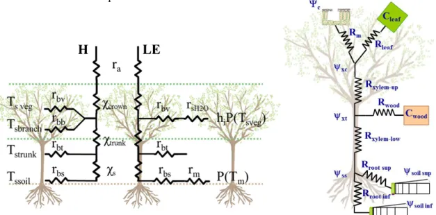
Figure 9. Diagrams of the energy budget and turbulent transfer resistance network and the tree hydraulic system. The Soil-Plant-Atmosphere continuum (SPAC) model couples stomatal conductance, water transport through the tree from the roots to the stomata, water uptake by roots, photosynthesis and CO2 soil fluxes and finally the tree energy balance (Figure 9). The stomatal conductance is computed with a modified Leuning's (1995) model and depends on photosynthesis and leaf water potential, allowing to link the stomatal conductance with the water flow in the tree and the soil water content. The hydraulic model describes the exchanges of water between the transpiration stream and the internal tree storage compartments via capacitive discharge and recharge (Figure 9). An additional mechanistic submodel of rainfall interception was included in order to more accurately model the water balance of the whole forest stand.

2.2.2. Adaptation of the model to an urban park with sparse linden trees

The soil-plant-atmosphere continuum model was designed for forest trees and an complete set of parameters was already acquired for beech trees. Yet, we saw that the city significantly modifies the soil and microclimate (Bozonnet et al., 2013), that is why some adjustments were necessary. We modified the parts on radiation, wind profile and soil structure to take into account firstly the fact that the garden is in a city and secondly that we have a sparse tree canopy with an underlying lawn.

The trees cover is sparse but we assume that the trees are closed enough for the roots to explore all the soil. Indeed, we have 50m2 _{of lawn for one tree, that represents a circle of 8m diameter and the crown} diameter is 5m. The trees are about 30 years old, so we can suppose that the roots are fully developed to explore all the volume homogeneously.

In addition, as the model is one-dimensional, we assume that the soil garden is fully coated with lawn. It is also possible to account for the surface of bitumen and bare soil by fixing a surface proportion for each type of soil cover, however to simplify our study, we only consider the lawn as soil cover.

The lawn roots explore the 0-30 cm soil layer, 70% of the tree roots are in the 30-100 cm layer and the 30% remaining are in the 1-2 m layer. The hydrodynamic characteristics depend on the soil texture which is sandy loam for the first meter and loamy sand between 1 and 2 m. In its last version, the model was parameterized for beeches, so we also need to adapt the tree structure and physiological characteristics to linden trees.

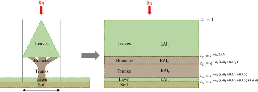
2.2.2.1. Adaptation of the radiation transfer model to take into account the sparse tree canopy As the model is calibrated for a forest (Tuzet et al., 2017), we consider a homogeneous tree cover. To take into account the fact that the tree crowns cover only 40% of the garden soil, we consider an exponential attenuation of the net radiation and we modified the attenuation coefficient k to obtain that 60% of the net radiation reach the lawn and 40% are intercepted by the tree crown. By resolving the equation: 𝑒+,-./0- = 0.6, we get for the tree canopy: 𝑘₆ = 0.125.

As the lawn is a homogeneous cover we take a different attenuation coefficient: 𝑘₇ = 0.5.

Figure 10. Scheme of the radiative transfer model used.

The Figure 10 represents the different layers with their leaf or wood area index and transmission functions. LAI_; is the tree leaf area index, BAI_> the branches area index, BAI_; the trunk area index and LAI? is the leaf area index of the lawn.

The net radiation in the different layers is computed as: 𝑅𝑛_7BCDBE = F1 − 𝑒+,-./0-H𝑅𝑛

𝑅𝑛_IJCKLMBE= F𝑒+,-./0-− 𝑒+,-(./0-NO/0P)H𝑅𝑛

𝑅𝑛6JQK, = F𝑒+,-(./0-NO/0P)− 𝑒+,-(./0-NO/0PNO/0-)H𝑅𝑛

𝑅𝑛_7CRK = F𝑒+,-(./0-NO/0PNO/0-)− 𝑒+(,-(./0-NO/0PNO/0-)N,S./0S)H𝑅𝑛 𝑅𝑛_ETU7 = 𝑒+(,-(./0-NO/0PNO/0-)N,S./0S) 𝑅𝑛

𝑅𝑛 Leaves Branches Trunks Lawn Soil 40% 𝑡W= 1 𝑡X= 𝑒+,-./0- 𝑡Y= 𝑒+,-(./0-NO/0P) 𝑡Z= 𝑒+,-(./0-NO/0PNO/0-) 𝑡[= 𝑒+,-(./0-NO/0PNO/0-)N,S./0S LAI; BAI> BAI; LAI? Rn Leaves Branches Trunks Lawn Soil

2.2.2.2. Calculation of the wind and eddy diffusivity profiles adapted to a sparse tree canopy in city The determination of the wind profile at the garden level is necessary to find the wind speed at every height from the wind measured at the reference height (𝑧_{JB_} = 17 m). Thanks to this wind profile and the associated exchange coefficient, we will also determine the turbulent transfer and boundary layer resistances that will be used in the model for the quantification of exchanges between the different compartments (part 2.2.2.3).

The wind profile will depend on the soil and obstacle geometry. In our case, we have two sparse canopies (building canopy and tree canopy) encased one inside the other. Indeed, we can see on the Figure 6 that the garden composed by lawn and sparse trees is surrounded by buildings.

The Figure 11 represents the scheme we used to describe the garden and the geometric features of the different elements (buildings, trees and lawn) are listed in the Table 2.

Figure 11. Scheme of the garden used to calculate the wind profile.

Table 2. Parameters related to the buildings, trees and lawn geometry Variable Value Unit Description

Buildings related information

ℎ_I 18 m Building average height

L 58 m Building average length

W 27 m Building average width

d 33 m Building average spacing

Trees related information

ℎ6JBB 9.2 m Average tree height

ℎ6JQK, 2.2 m Average trunk height

𝑅_6JQK, 0.19 m Average trunk radius 𝑅_LJTRK 2.52 m Average crown radius 𝑆LJTRK 20 m2 Crown projected surface

𝑆_7CRK 52 m2 _{Area of lawn per tree}

𝐿𝐴𝐼_6JBB 11.2 m2_.m-2 _{Leaf area index of one tree} Lawn related information

ℎ7 0.10 m Average grass height

𝐿𝐴𝐼_7CRK 3 m2_.m-2 _{Lawn leaf area index}

The wind profile is decomposed in four parts: - Above the buildings (𝑧 ≥ 18𝑚)

- Between the top of the trees and the top of the buildings (9.2 ≤ 𝑧 ≤ 18𝑚 ) - Between the top of the lawn and the top of the trees (0.10 ≤ 𝑧 ≤ 9.2𝑚 ) - In the lawn (𝑧 ≤ 0.10𝑚 )

o We first consider a logarithmic wind profile at the city level, above the buildings: 𝑢(𝑧) =𝑢∗L

𝜅 ln o 𝑧 − 𝑑_L

𝑧_qL r

With 𝑢_∗L the friction velocity at the city level (m.s-1_{), 𝜅 the Von Karman constant (𝜅 = 0.4), 𝑧 the height} (m), 𝑑_L the displacement height relative to the city (m) and 𝑧_qL the roughness height relative to the city (m).

From the logarithmic wind profile above the city, the turbulent transfer coefficient is calculated as: 𝐾(𝑧) = 𝜅 𝑢_∗L(𝑧 − 𝑑_L)

We estimated the roughness and displacement height of the city with the method of Grimmond and Oke (1999). They modified the equation of Macdonald et al. (1998) and found an expression of the displacement height (𝑑_L, m) and the roughness length (𝑧_qL, m) normalized by the obstacle height (ℎ_I, m) available for urban canopy:

uv MP= 1 + 𝐴 +xy(𝜆 {− 1) and |_M}v_P = ~1 −u_MPv• 𝑒𝑥𝑝 o− ~0.5𝛽ƒ_…„†~1 − uv MP• 𝜆‡• +q.[ r

Where 𝐴 is an empirical constant (𝐴 = 4), 𝐶_‰ is the drag coefficient (𝐶_‰= 1.2) and 𝛽 is a corrective factor (𝛽 = 1). The ratio uv

MP depends on the plan aspect ratio roughness density (𝜆{− m

2_.m-2_{) and} |}v

MP depends on the frontal aspect ratio roughness density (𝜆_‡− m2_.m-2_).

𝜆{ is calculated as : 𝜆{=/_/y

Š and 𝜆‡ as: 𝜆‡ =

/‹

/Š . Where 𝐴_‡ is the frontal area of roughness elements (m2_{), 𝐴}

{ is the plan area of roughness elements (m2)

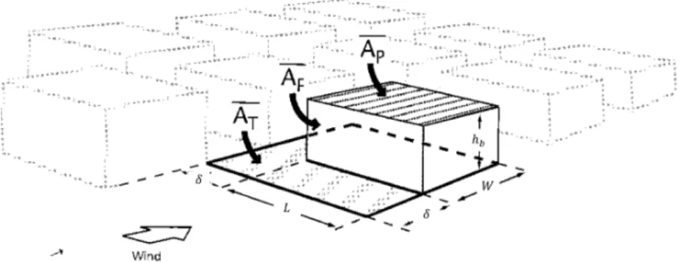
and 𝐴_Œ is the plan area of total surface (m2_{). The Figure 12 shows how Grimmond and Oke (1999)} computed these different areas in their study. They use a simplified and homogenous building topology, in real cities the topology is obviously more complex, but we tried to comply with this simplified scheme by taking the average building dimensions.

Figure 12. Definition of surface dimensions used in morphometric analysis (modified from Grimmond and Oke, 1999). The different areas are calculated as: 𝐴_{= 𝐿 × 𝑊, 𝐴_‡ = ℎ_I× 𝐿 𝑎𝑛𝑑 𝐴_Œ = (𝛿 + 𝐿) × (𝛿 + 𝑊).

Where 𝐿, 𝑊 and 𝛿 are respectively the average building length, width and spacing in meter (we consider the same average spacing on each side of the buildings).

In order to calculate the density obstacle of our site, we took into account the areas around the garden and the DRIRE building which is representative of the University district of Strasbourg. The different lengths and heights were measured with the tools ImageJ and BD TOPO®. The results are presented in Table 3.

Table 3. Results of the calculated parameters to obtain the displacement and roughness heights

Parameter Value Unit Description

𝐴_{ 1566 m2 _{Plan area of roughness elements}

𝐴_‡ 1044 m2 _{Frontal area of roughness elements}

𝐴_Œ 5460 m2 _{Plan area of total surface}

𝜆_{ 0.29 m2_.m-2 _{Plan aspect ratio of roughness density} 𝜆‡ 0.19 m2.m-2 Frontal aspect ratio of roughness density

𝑑_L 9.37 m Displacement height at the top of the city

𝑧_qL 1.57 m Roughness length at the top of the city

o Secondly, we will use the model developed by Wang (2012) to calculate the wind profile in a sparse canopy.

For sparse and dense canopy, a wind exponential attenuation is usually used (Kaimal and Finnigan, 1994), however in sparse canopy the wind is often less attenuated and the wind profile needs to be adjusted. Wang (2012) takes into account the effects of both the ground and canopy elements on turbulent mixing and proposes a new wind profile more suitable for sparse canopy.

In our study case we saw that we can consider two different encased canopies. Indeed, we can consider the city buildings as a first sparse canopy and the garden trees as a second sparse canopy. Therefore, we will use the Wang’s model twice. First we will calculated the wind profile in the building canopy without trees and then we will consider the tree canopy within the building sparse canopy ensuring of course, the continuity of the wind profile at the top of the trees. In the following part we will present the equations which are the same for both building and tree canopies, and then we will take into account the parameters related to the buildings and the trees to get different wind profiles.

Wang (2012) considers the momentum transfer equation with some assumptions that will allow him to solve it: − 𝜕 𝜕𝑧“𝐾 𝜕𝑈(𝑧) 𝜕𝑧 • = − 1 𝜌 𝜕𝑃 𝜕𝑥− 𝐶.𝑎q𝑈(𝑧)𝑈M 𝑤𝑖𝑡ℎ 𝐾(𝑧) = 𝜅𝑧𝑠M𝑢∗L

Where 𝐾(𝑧) is the eddy diffusivity, 𝑠_M is a factor representing the effect of canopy elements on the length scale and 𝑢_∗L is the friction velocity above the canopy, therefore 𝐾 is proportional to 𝑧. To find s_œ, we can say that at 𝑧 = ℎ_I, the turbulent transfer coefficients are equal so:

𝐾(ℎ_I) = 𝜅𝑠_M𝑢_∗L ℎ_I= 𝜅 𝑢_∗L (ℎ_I− 𝑑_L) Þ 𝑠_M = 1 −uv

Then, using the modified Bessel functions, a solution of the momentum equation is given by: 𝑈(𝑧) = 𝐶_W𝐼_qF𝑔(𝑧)H + 𝐶_X𝐾_qF𝑔(𝑧)H + 𝑈_{ with 𝑔(𝑧) = 2ž𝛼_M|

Where 𝐼_q and 𝐾_q are the modified Bessel functions of the first and second kinds of order 0, ℎ is the canopy height, 𝛼 is a attenuation coefficient calculated from the frontal area index (𝜆‡) as: 𝛼 =

4.52 𝜆_‡+ 0.62 𝜆_‡X. Wang overlooks the pressure variation term so 𝑈_{= 0. 𝐶_W and 𝐶_X are integration coefficients that can be determined with the boundary conditions: 𝑈F𝑑₇+ 𝑧_q7H = 0 and 𝑈(ℎ) = 𝑈_M, where 𝑑₇ and 𝑧_q7 are respectively the roughness and displacement heights of the lawn. 𝐶_W and 𝐶_X are given by:

𝐶_W= ¡+ yN y¢}(£(M))/¢}(£FuSN|}SH)

0}F£(M)H+0}(£FuSN|}SH)¢}(£(M))/¢}(£FuSN|}SH) and 𝐶X=

yNƒ¥0}(£FuSN|}SH)

¢}(£FuSN|}SH)

The roughness and displacement heights of the lawn are estimated with the method of Perrier (1982) for homogeneous plant canopy:

𝑑₇ = ¦1 − 2 𝐿𝐴𝐼£JCEE“1 − 𝑒 +./0§¨©ªª_{X •« × ℎ} 7CRK 𝑧_q7 = ¦“1 − 𝑒+./0§¨©ªªX • . 𝑒+ ./0§¨©ªª X « × ℎ_7CRK We find 𝑧q7 = 0.048 m and 𝑑7 = 0.017 m.

Table 4. Parameters used in the calculation of the Wang’s wind profile for buildings and trees canopies

Parameter Buildings Trees

ℎ (𝑚) 18 9.2

𝜆‡ (𝑚X. 𝑚+X) 0.19 0.35

𝛼 (−) 0.89 1.68

Figure 13. Combined wind profiles in the buildings and trees canopies.

0 2 4 6 8 10 12 14 16 18 0.0 0.2 0.4 0.6 0.8 1.0 z (m ) u(z)/u(18) (m/s) u(z) buildings canopy

u(z) trees canopy

These calculations are available for the buildings and the trees canopies. Through the parameters α and ℎ (Table 4), we will take into account the topology of the canopy and obtain different wind profiles (Figure 13).

o In the lawn, we consider an exponential attenuation of the wind due to the absorption of the momentum by the grass leaves:

𝑢(𝑧) = 𝑢(ℎ7)𝑒𝑥𝑝 ¦𝛼7o

𝑧

ℎ7− 1r«

Where α₇ (unitless) is the attenuation coefficient taken equal to 2.5 for dense canopy (Kaimal and Finnigan, 1994).

As we saw previously, the wind profile is calculated in four parts, then we assure the profile continuity at each junction (Figure 14).

Figure 14. Diagram of the garden and the associated final wind profile.

With this wind profile approach, we can calculate the proportionality coefficient connecting the measured roof and garden wind values and compare it with the one obtained experimentally.

We get 𝑢(17) = 0.71 𝑢(25), this result is in the same order of magnitude as the experimental coefficient that we got from the linear regression (Figure 8), therefore this theoretical reasoning justifies the fact that the wind speed in the garden is significantly attenuated. To fill the missing data we will use a coefficient of 0.64 to multiply the wind speed at 25m.

Logarithmic profile above the city

Wind attenuation due to the buildings

z = 18m

Wind attenuation in the tree crown

Wind attenuation in the lawn z = 9.2m u(z) city u(z) trees u(z) buildings u(z) lawn Garden mast 17m

Figure 15. Resistive scheme used in the model and for the calculation of the climatic demand and maximum evapotranspiration of the cover

2.2.2.3. Computation of the resistances

2.2.2.3.1. Analytical expressions of the aerodynamical and turbulent transfer resistances All the aerodynamical and turbulent transfer resistances are calculated as:

𝑅 = ∫

|† where 𝐾(𝑧) is the eddy diffusion coefficient. This coefficient depends on the altitude 𝑧 and has different expressions according to the wind profile considered. As a reminder:

- Above the buildings (z ≥ ℎI), we have a logarithmic wind profile and 𝐾(𝑧) = 𝜅 𝑢∗L(𝑧 − 𝑑L).

- Between the top of the trees and the top of the buildings (ℎ6JBB≤ z ≤ ℎI), our wind profile is

describe by Wang (2012) and the eddy diffusion coefficient is expressed as: 𝐾(𝑧) = κzsœu∗´.

- Between the top of the lawn and the top of the trees (ℎ7 ≤ z ≤ ℎ6JBB), we use the same

expression of 𝐾(𝑧) corresponding to the other sparse canopy.

- Between the roughness length of the soil and the top of the lawn (𝑧qETU7 ≤ z ≤ ℎ7), we consider

an exponential attenuation of the wind speed and of the eddy diffusion coefficient with the same attenuation coefficient (α7 = 2.5): 𝐾(𝑧) = 𝐾(ℎ7)𝑒𝑥𝑝 “𝛼7~_M|

S− 1••.

The expressions of the aerodynamical and turbulent transfer resistances are detailed in the Appendix 2. The computation of the resistances results from the

expression of the wind profile, they will be used in the model to quantify exchanges between the different compartments. The Figure 15 shows the different resistances where:

𝑅_C-is the aerodynamical resistance above the tree canopy,

𝑅_6JBBª and 𝑅_6JBBµ are the turbulent transfer resistance in the upper and lower parts of the canopy,

𝑅6JQK,ª and 𝑅6JQK,µ are the turbulent transfer resistance in the upper and lower parts of the trunks, 𝑅_7CRKª and 𝑅_7CRKµare the turbulent transfer resistance in the upper and lower parts of the lawn, 𝑟_IS·©¸·ª, 𝑟_{IP¨©¹v¡·ª}, 𝑟_I-¨º¹», 𝑟_IS©¼¹ and 𝑟_£ are respectively the leaves, branches, trunk, lawn and soil boundary layer resistances.

𝑧JB_ ℎ6JBB ℎ½ 6JBB ℎ6JQK, ℎ½ 6JQK, ℎ7CRK ℎ½ 7CRK 𝑧_qETU7 𝑅_𝑎𝑡 𝑟_{𝑏𝑙𝑒𝑎𝑣𝑒𝑠} 𝑅𝑡𝑟𝑒𝑒𝑠 𝑅_{𝑡𝑟𝑒𝑒𝑖} 𝑟_{𝑏𝑏𝑟𝑎𝑛𝑐ℎ𝑒𝑠} 𝑅_{𝑡𝑟𝑢𝑛𝑘𝑠} 𝑟_{𝑏𝑡𝑟𝑢𝑛𝑘} 𝑅_{𝑡𝑟𝑢𝑛𝑘𝑖} 𝑅_{𝑙𝑎𝑤𝑛𝑠} 𝑟𝑔 𝑟_{𝑏𝑙𝑎𝑤𝑛} 𝑅_{𝑙𝑎𝑤𝑛𝑖}

2.2.2.3.2. Computation of the boundary layer resistances

The different boundary layer resistances are calculated with the expression of Schuepp (1972) and Finnigan and Raupach (1987) as:

𝑟_I = h 𝐿𝐴𝐼 Â

𝐷 𝑢(ℎ_½)

Where 𝐷 is a length characteristic (m), h is an empirical coefficient (h= 76.84), 𝐿𝐴𝐼 or 𝐵𝐴𝐼 is the leaf of branch area index (m_{7BCDBE TJ IJCKLMBE}X _{. m}

ETU7

+X _{) and 𝑢(ℎ}

½) is the wind speed at the altitude ℎ½

corresponding to the half-height of the considered cover.

The parameters 𝐷, ℎ_½ and 𝐿𝐴𝐼 or 𝐵𝐴𝐼 depends on the type of surface considered (leaves, branches ...) and are presented in the Table 5.

Table 5. Parameters used to calculate the different boundary layer resistances

Resistance D (m) h_Ç (m) 𝐿𝐴𝐼 or 𝐵𝐴𝐼 (m2_.m-2₎

𝑟IS·©¸·ª Leaves boundary layer resistance 0.075 5.7 4

𝑟_{IP¨©¹v¡·ª} Branches boundary layer resistance 0.11 5.7 1.18

𝑟_I-¨º¹» Trunk boundary layer resistance 0.38 1.05 0.05

𝑟IS©¼¹ Lawn boundary layer resistance 0.005 0.05 3

The branches and trunks boundary layer resistances are used in the model, however, they are not introduced in the next part for the calculation of the climatic demand and maximum evapotranspiration because we neglect the branches and trunks transpiration.

Finally, the soil boundary layer resistance is always very high and fixed equal to: 𝑟_I = 1000 s. m+W_.

2.3. Calculation of the climatic demand and maximum evapotranspiration

In order to analyze the hydric state of trees and grass, we compare the measurements of latent heat flux (evapotranspiration) with calculated indicators as climatic demand and maximum evapotranspiration.

2.3.1. Calculation of the climatic demand

By definition, the climatic demand or the potential evapotranspiration (PE, W.m-2_{) is the amount of} evapotranspiration of a surface when the water is fully available (i.e. the surface is covered by a thin film of water).

The climatic demand is calculated as: 𝑃𝐸 = {É

{É_NÊ“(𝑅𝑛 − 𝐺) +

̃Í

J©NJ

ª-¨ºv-{(Œ©)+{(Œ¨)

{É •

Where 𝑅𝑛 is the net radiation (W.m-2_{), 𝐺 is the heat conduction flux in the soil (W.m}-2_{), 𝑃}Î _{is the slope}

of the curve of the partial pressure of water vapor (Pa.°C-1_{). 𝑟}

C is the aerodynamical resistance (s.m-1),

𝑟_E6JQL6 is the structure resistance of the plant cover (s.m-1_{), 𝛾 is the psychrometric constant 𝛾 = 66} Pa.°C-1_{, 𝜌 is the air bulk density (𝜌 =1.2 kg.m}-3_{) and 𝐶}

Ð is the air specific heat capacity (𝐶Ð=1015 J.kg

The climatic demand calculation requires to quantify the radiative and convective terms. To do that, we will use the measured weather forcing data and the calculated resistances associated with the wind profile in the garden (part 2.2.2.2).

The resistive scheme used in the calculation of the convective term of the climatic demand is presented in Figure 15. For the computation of the total climatic demand (trees + lawn), the aerodynamical resistance is equal to 𝑅_C6 and for the lawn climatic demand, as we used the measurements carried out at 2m and the aerodynamical resistance is equal to 𝑅_6JQK,U+ 𝑅_6JQK,E.

In order to determine the structure resistance, we do an analogy with the Ohm law in order to calculate an equivalent resistance of the cover:

For the lawn : 𝑟_{E6JQL6 7CRK} = 𝑅_7CRKE+ JPS©¼¹ ¨PS©¼¹ ÑS©¼¹µÒ¨§NW

For the overall garden: 𝑟_{E6JQL6 £CJuBK} = 𝑅_6JBBE+ JPS·©¸·ª ¨PS·©¸·ª

Ñ-¨··µÒÑ-¨º¹»µÒÑ-¨º¹»ªÒ¨ª-¨ºv- S©¼¹NW

2.3.2. Calculation of the maximum evapotranspiration

The maximum evapotranspiration (ETM, W/m2_{) is the amount of evapotranspiration of a plant assuming} that the leaf stomata are completely open because the soil is well supplied with water (i.e. the stomatal resistance is minimum):

𝐸𝑇𝑀 =

WN Ù

yÉÒÙ ¨ªÚµ¹ vÛ¸·¨

¨©Ò¨ª-¨ºv-

The minimal stomatal resistances for Tilia Tomestosa Moench and for the lawn were estimated from values given in the literature.

• For Tilia Tomestosa Moench: 𝑔E½CÜ = 0.004 m.s-1 (Bournez, 2018)

𝑟_{E ½UK 7BCDBE}= 1 𝑔_E½CÜ= 1 0.004= 250 𝑠. 𝑚+W 𝑟 E ½UK LTDBJ Ý J_./0ª S·©¸·ª -¨·· Ý X[qZ ÝÞX.[ E.½ ߥ

• For the lawn: 𝑔_Eƒà†= 0.65 mol.m-2_.s-1 _{(Manea and Leishman, 2014)} 𝑟E ½UK 7BCDBE= 𝑃_C6½ 𝑅𝑇CUJ× 0.64 𝑔Eƒà† = 41 𝑠. 𝑚+W 𝑟 E ½UK LTDBJ Ý J_./0ª S·©¸·ª §¨©ªª Ý ZWY Ý WY.á E.½ ߥ

With 𝑇_CUJ = 293 K, 𝑃_C6½= 1013. 10X _{Paand 𝑅 = 8.314 J. mol}+W_{. K}+W _{(perfect gas constant).}

To calculate the climatic demand and maximum evapotranspiration of the park (trees + lawn) we use the resistances described in the part 2.2.2.3 and the net radiation, air temperature and partial pressure of water vapor at 17m.

3. Results and discussion

3.1. Analysis of the experimental results

We decided to focus on the analysis of the two years 2014 and 2015 which have different rainfall. We focus more particularly on the tree vegetative period which is from April to October. In this part, we will first describe and compare the two-year climate, then we will analyze the tree and lawn transpirations, and finally these transpiration measurements will be compared with the calculated climatic demand and maximum evapotranspiration.

3.1.1. Description and comparison of the 2014 and 2015 climate

In order to compare the climate of the two years, we analyzed the precipitation rate and the climatic demand. The latter combines radiative and convective terms in its calculation.

Figure 16. Cumulated annual (left) and monthly (right) precipitation in 2014 and 2015

On the Figure 16, we can see that during the first half of the year, 2014 was dryer that 2015 which is closed to the average precipitation rate. However, in July we observe an inversion. In July 2014 we observe heavy rainfall (200 mm) that compensate the spring hydric deficit, while June and July 2015 were very dry (50 mm in two months), and finally at the end of the year we observe a hydric deficit of 164 mm compare to the 1981-2018 average.

In addition, the initial stock of water in soil at the beginning of our studied period (April, 1st_{) is very} closed for both years (0.137 m3_.m-3 _{in 2014 and 0.143 m}3_.m-3 _{in 2015) and it will vary over the year} with precipitation and vegetation transpiration rate.

Thanks to these data, we can foresee a potential water stress for the vegetation in the 2014 spring and 2015 summer and fall.

0 50 100 150 200 250 1 2 3 4 5 6 7 8 9 10 11 12 Mo nt hl y pr ec ip ita tio n (m m ) Month 2014 2015 Monthly average 1981-2018

Figure 17. Cumulated climatic demand for the whole garden in 2014 and 2015

To help us in our analysis, we calculated the climatic demand (PE) from the climate data measured in the garden (part 2.3.1). The PE of the whole garden is presented in Figure 17, where we observe that like the precipitation, we have a turning point in the middle of July. However, unlike the rainfall, the climatic demand is larger in 2015 than in 2014. Indeed, we can assume that in 2015, as there is less rain, there is less clouds and therefore more net radiation. The temperature may also be higher with a lower relative humidity inducing a larger hydric deficit.

To find which meteorological variable is responsible of the difference in the climatic demand, we plot in Figure 18 the convective and radiative terms of the climatic demand. We notice that the radiative terms are very closed for the two years and the convective terms seem to explain the difference of climatic demand. It can be due to a difference of wind speed (through the aerodynamical or turbulant transfer resistances) or of hydric deficit. We noticed no difference of the average wind speed of the two years, but if we look at the cumulated hydric deficit which is plotted in Figure 19, this confirms that it is the cause of the different climatic demand. The weather in the 2015 summer was warmer and less humid, inducing a larger hydric deficit and so a larger climatic demand. Figure 18. Cumulated convective and radiative terms of the

total climatic demand in 2014 and 2015.

3.1.2. Trees and grass evapotranspiration

All the latent heat fluxes are brought back to the grass surface by accounting for the different surface proportions which are presented in the Table 6 (these different surface were calculated with an aerial photography of the garden and the software ImageJ and the tree crown does not account in the soil total surface).

Figure 20. Cumulated measured tree latent heat flux in 2014 and 2015. Figure 21. Volumetric soil water content in the 30-100cm layer in 2014 and 2015.

We observe on the Figure 20 that until the end of June, the tree transpiration rates are very closed for both years. Then, despite the potential water stress due to the lack of rainfall in June and July 2015, the tree transpiration seems high in 2015. To compensate the limited precipitation, the soil water content should be higher in 2015. However we see on Figure 21 that it is not the case, while the important rainfalls of July 2014 induce an increase of the soil water content, it continues to decrease in 2015. Finally, in spite of the lower precipitation and soil water content, the tree water stress in 2015 appears to be limited. We can assume that as the city of Strasbourg is crossing by many watercourses the groundwater may be at a few meters from the soil surface and therefore the trees are able to draw water in it. According to the Observatory of the Alsace water table (APRONA), that registers the groundwater level, in 2014 and 2015 the groundwater was in average at 135.8m above the see level and knowing that the level of the garden is about 138m, the groundwater is therefore at about 2m deep and could be reached by tree roots. Beside, over the two-year period the variation of the water table were limited with only 30cm between the maximum and the minimum level.

To analyze the lawn transpiration, we use the measurements carried out during a few days in 2014 and 2015. We added to these results the tree and total garden transpiration.

0. 00 0. 04 0. 08 0. 12 0. 16 0. 20

avr mai juil sept oct

So il w at er c on te nt (m 3.m -3) Date

Soil water content in the 30-100cm soil layer

2014 2015 Surface area m2 _% Tree 20 27 Lawn 50 67 Bitumen 11.5 15 Bare soil 13.5 18 Total area 75 100

Figure 21. Volumetric soil water content in the 30-100cm layer in 2014 and 2015.

Figure 20. Cumulated measured tree latent heat flux in 2014 and 2015.

Table 6. Calculated areas of the different surfaces for one tree.

Figure 22. Comparison of the measured latent heat fluxes of the trees (LE tree), grass (LE grass) and the whole garden (LE sonic) for different days in 2014 and 2015.

The error bars correspond to two times the standard deviation of the latent heat flux measured from the sap flows of six trees.

The Figure 22 represents the daily variation of the tree, lawn, and whole garden latent heat flux (LE). As a reminder, the tree transpiration is calculated from sap flow measurements, the lawn and soil evapotranspiration with transpiration chambers and the total latent heat flux of the garden with a sonic gas analyzer only in 2015.

There are two lawn latent heat fluxes resulting from two transpiration chambers, the chamber 1 is located in the middle of the garden while the chamber 2 is closer to the trees. We notice that the two evapotranspiration rates are closed except on the morning, when the transpiration rate of the chamber 2 is lower than the chamber 1 rate. It can be explained by the tree shade that limits the lawn and soil evapotranspiration.

The weak lawn LE on the 19th _{of June could be explained by the very low precipitation rate of June 2014} (17.4 mm against 73.5 mm on average - Figure 16).

-50 50 150 250 350 450 0:00 6:00 12:00 18:00 0:00 LE (W /m 2)

Hour of the day

19/06/2014

0:00 6:00 12:00 18:00 0:00 Hour of the day

16/07/2014

0:00 6:00 12:00 18:00 0:00 Hour of the day

01/08/2014 -50 50 150 250 350 450 0:00 6:00 12:00 18:00 0:00 LE (W /m 2)

Hour of the day

01/07/2015

0:00 6:00 12:00 18:00 0:00 Hour of the day

16/07/2015

0:00 6:00 12:00 18:00 0:00 Hour of the day

03/08/2015

If we compare the two years, we observe that the evapotranspiration of the lawn plus the soil is higher in 2014 with about 250 W.m-2 _{at midday while in 2015 a maximum of 173 W.m}-2 _{is reached on the 1}st of July. Then, in the middle of July and beginning of August the lawn LE is decreasing up to 50 W.m-2_. In view of this decline, we think that the lawn is under water stress and is probably dying, therefore this value of 50 W.m-2 _{correspond mostly to the soil evaporation.}

If we look at the tree transpiration, thanks to the standard deviation bars, we can first notice that there is a quite large difference within the six trees. Then we remark that the tree transpiration is rather constant over the year ; over the day, between 9am. and 4pm. the tree LE reaches a plateau which is in average 20W.m-2 _{higher in 2015. We can also notice a slight depression around midday probably due to the} stomata closure. We can also say that in non-limiting water conditions the soil and lawn evapotranspiration is higher than the tree transpiration.

The latent heat flux of the whole garden is measured on the 17m mast located at the center of the garden, its footprint is estimated at 2400m2 _{(Bournez, 2018). If we calculate the sum of the latent heat fluxes of} the trees and grass, we get a different result than the LE measured on the mast. The relative difference between the sonic LE and the sum of trees LE plus lawn LE varies from 0 to 40%, the bigger differences are observed during the midday peak. It can be explained by the presence of higher trees next to the buildings (see aerial picture Figure 6). Indeed, it is difficult to estimate precisely the footprint of sonic measurements and the sensor probably measures also the transpiration rate of the surrounding vegetation.

3.1.3. Comparison of the calculated climatic demand and maximum evapotranspiration with the measured latent heat fluxes

In this part, we pursue our analysis with the comparison of the tree and lawn evapotranspiration measurements and the calculated climatic demand and maximum evapotranspiration.

Figure 23. Comparison of the tree measured latent heat flux with the calculated climatic demand and maximum evapotranspiration for different days in 2014 and 2015.

The error bars correspond to two times the standard deviation of the latent heat flux measured from the sap flows of six trees.

The daily variation of the tree climatic demand, maximum evapotranspiration and latent heat flux is presented in Figure 23. We observe that at about 8am., the tree LE is equal to the maximum evapotranspiration, we can assume that the leaves are recovered by dew water and the stomatal resistance is minimum. Then the climatic demand and maximum evapotranspiration increase but the tree transpiration reaches a plateau and stay almost constant until 3pm, so we can say that there is a stomatal regulation. The climatic demand and maximum evapotranspiration attain a peak quite late in the day (around 5 pm.) and drop.

-50 50 150 250 350 450 550 0:00 6:00 12:00 18:00 0:00 LE (W /m 2)

Hour of the day

19/06/2014

0:00 6:00 12:00 18:00 0:00 Hour of the day

16/07/2014

0:00 6:00 12:00 18:00 0:00 Hour of the day

01/08/2014 -50 50 150 250 350 450 550 0:00 6:00 12:00 18:00 0:00 LE (W /m 2)

Hour of the day

01/07/2015

0:00 6:00 12:00 18:00 0:00 Hour of the day

16/07/2015

0:00 6:00 12:00 18:00 0:00 Hour of the day

03/08/2015

Figure 24. Comparison of the lawn measured latent heat flux with the calculated climatic demand and maximum evapotranspiration for different days in 2014 and 2015.

As in the Figure 22, we see in the Figure 24 that the lawn and soil evapotranspiration increases in the 2014 summer and decreases in 2015. However, the ETM is almost the same over the summer, so there is a strong stomatal regulation due to the lawn water stress. We can conclude that in June 2014 and in July and August 2015 the lawn limits its transpiration because soil water content is reduced and that provokes a progressive death of the lawn. In addition, the lawn may be more sensible to water stress because unlike trees, it is unable to draw water at several meters deep.

Thanks to these results, we can forecast that the linden trees may draw water in the groundwater table and are less sensible to the water-limited conditions, on the contrary, the lawn seems to be under water stress on the first half of the year 2014 and the second half of 2015.

In the simulation part, we will try to take in account in the model the fact that the trees draw in a water table and that the lawn progressively dies due to water stress.

-50 50 150 250 350 450 550 0:00 6:00 12:00 18:00 0:00 LE (W /m 2)

Hour of the day

19/06/2014

0:00 6:00 12:00 18:00 0:00 Hour of the day

16/07/2014

0:00 6:00 12:00 18:00 0:00 Hour of the day

01/08/2014 -50 50 150 250 350 450 550 0:00 6:00 12:00 18:00 0:00 LE (W /m 2)

Hour of the day

01/07/2015

0:00 6:00 12:00 18:00 0:00 Hour of the day

16/07/2015

0:00 6:00 12:00 18:00 0:00 Hour of the day

03/08/2015

3.2. Results of the simulation

In the previous part, the analysis of the experimental results with the calculation of the climatic demand and the maximum evapotranspiration enabled us to better understand the hydraulic functioning of the urban trees and lawn in water stress conditions. In this part, we will present the results of the simulations obtained with the SPAC model and compare them with the experimental measurements. We will see than the model can give more information on the latent heat flux distribution between the different elements composing the garden.

3.2.1. Comparison of the modeled and measured tree transpiration

First we will compare and analyze the results of the simulated and measured tree transpiration before the insertion of a groundwater in the model.

Figure 25. Comparison of the model results with the experimental measurements in 2014 and 2015

Compare to the measurements, we see on the Figure 25 that the model underestimates the tree transpiration in the 2014 spring and in 2015 from July and the difference is very large in the second half of 2015. These periods corresponds to relatively dry periods, when the model registers a water stress for trees. This water stress is overestimated by the model, and this confirms the hypothesis we made in the conclusion of the previous part, that is to say that the trees transpiration is not limited by the relatively low soil water content and therefore they probably draw water in the groundwater which is few meters deep.

To improve our simulations, we take into account this groundwater in our model by adding a saturated soil layer at 2 m deep. The hydraulic resistance of fine roots connecting the water table to large roots is assumed constant in this first approach. Values taken in 2014 and 2015 are different because we assume that in water-limited conditions the tree is able to develop fine roots at the interface between soil and groundwater and to increase its capacity to draw in the water table (𝑅_XqWZ= 75 × 10Þ _{MPa. m}+W_{. s and}

3.2.2. Improvement of the simulations thanks to the modelling of a groundwater

Figure 26. Comparison of the model results and the experimental measurements with the introduction of a water table in 2014 and 2015

The Figure 26 shows the tree transpiration after the introduction of a groundwater in the model. We observe that the simulations fit better the measurements than without the groundwater (Figure 25). The slight over or underestimations may be due to the arbitrary fixed water table hydraulic resistances.

Figure 27. Tree leaves water potential with and without a water table in 2014 (left) and 2015 (right).Tree leaves water potential with and without a water table in 2014 (left) and 2015 (right).

If we look at the leaves water potential (Figure 27), we can first notice that for both years during the water-limited periods and without the groundwater, the potentials (black lines) drop to higher negative values inducing a lower water flux (i.e. transpiration). The introduction of a groundwater prevents the drop of the potential (blue line) and therefore increases the tree transpiration. We can also say that when the water is not limited the potential values are very closed meaning that the trees are not drawing in the groundwater.

If we compare 2014 and 2015 with the groundwater (blue curve), we observe that during the water-limited periods, the potential slightly decrease in 2015 compare to the higher potential drop we observe in 2014. This is probably due to the higher hydraulic resistance that we fixed in 2014.

Finally, we can conclude that the introduction of a saturated soil layer to represent a groundwater in the model allows the tree transpiration to be less sensible to variations of soil water content and is congruent with the experimental measurements.

3.2.3. Analysis of the latent heat flux of the different elements and comparison simulations - measurements

As we have only daily measurements of lawn and soil evapotranspiration, the results of the model can help us to understand the sharing of the latent heat flux between the trees, lawn and soil. This distribution is presented on the Figure 28.

Figure 28. Modeled tree, lawn an soil latent heat fluxes in 2014 (left) and 2015 (right)

In 2014, before July the grass transpiration is higher and then the tree transpiration becomes greater (Figure 28). It can be explained by the fact that we limited the drawing in the groundwater in 2014 and that until July the low rainfall observed only contributes to re-moistening the upper layer of soil; this layer corresponds to the volume of soil used by the grass roots. The deeper layers in which tree roots draw receive almost no water.

To take into account the lawn death due to water stress, we separate the lawn LAI in two parts one green and one dry, we increase the dry LAI from the 9th of June 2015 with a logistic function decreasing until 0.4. The total LAI is thus the sum of the green and dry LAI and is always equal to 3. Then, the stomatal conductance is multiplied by the ratio ./0

¸·¨-./0-Û-©S (which decreases from 1 to 0.13). This decrease of stomatalconductance induces a reduction of the transpiration in 2015 as we can observe on the Figure 28.

However this method of LAI decrease was not applied to the radiative budget and wind profile calculations. That is why the soil which is not more exposed to radiative energy and wind nearly has the same evaporation for both years.

Thanks to the measurements in transpiration chambers, we can compare the measured and modeled lawn plus soil latent heat flux. The Figure 29 presents the daily lawn and soil LE the tree transpiration and also the total garden evapotranspiration.