HAL Id: hal-01479532
https://hal-amu.archives-ouvertes.fr/hal-01479532
Submitted on 7 May 2018
HAL is a multi-disciplinary open access
archive for the deposit and dissemination of
sci-entific research documents, whether they are
pub-lished or not. The documents may come from
teaching and research institutions in France or
abroad, or from public or private research centers.
L’archive ouverte pluridisciplinaire HAL, est
destinée au dépôt et à la diffusion de documents
scientifiques de niveau recherche, publiés ou non,
émanant des établissements d’enseignement et de
recherche français ou étrangers, des laboratoires
publics ou privés.
Combining Restarts, Nogoods and Bag-Connected
Decompositions for Solving CSPs
Philippe Jégou, Cyril Terrioux
To cite this version:
Philippe Jégou, Cyril Terrioux. Combining Restarts, Nogoods and Bag-Connected Decompositions for
Solving CSPs. Constraints, Springer Verlag, 2017, 22(2) (2), pp.191-229. �10.1007/s10601-016-9248-8�.
�hal-01479532�
Combining Restarts, Nogoods and
Bag-Connected Decompositions for Solving CSPs
∗
Philippe J´
egou
Cyril Terrioux
Aix Marseille Universit´e, CNRS, ENSAM, Universit´e de Toulon,
LSIS UMR 7296, 13397 Marseille, France
{philippe.jegou,cyril.terrioux}@lsis.org
Abstract
From a theoretical viewpoint, the (tree-)decomposition methods offer a good approach for solving Constraint Satisfaction Problems (CSPs) when their (tree)-width is small. In this case, they have often shown their prac-tical interest. So, the literature (coming from Mathematics, OR or AI) has concentrated its efforts on the minimization of a single parameter, namely the tree-width. Nevertheless, experimental studies have shown that this parameter is not always the most relevant to consider when solving CSPs. So, in this paper, we highlight two fundamental problems related to the use of tree-decomposition and for which we offer two particularly appro-priate solutions. First, we experimentally show that the decomposition algorithms of the state of the art produce clusters (a tree-decomposition is a rooted tree of clusters) having several connected components. We high-light the fact that such clusters create a real disadvantage which affects significantly the efficiency of solving methods. To avoid this problem, we consider here a new graph decomposition called Bag-Connected Tree-Decomposition, which considers only tree-decompositions such that each cluster is connected. We analyze such decompositions from an algorith-mic point of view, especially in order to propose a first polynomial time algorithm to compute them. Moreover, even if we consider a very well suited decomposition, it is well known that sometimes, a bad choice for the root cluster may significantly degrade the performance of the solv-ing. We highlight an explanation of this degradation and we propose a solution based on restart techniques. Then, we present a new version of the BTD algorithm (for Backtracking with Tree-Decomposition [28]) in-tegrating restart techniques. From a theoretical viewpoint, we prove that reduced nld-nogoods can be safely recorded during the search and that their size is smaller than ones recorded by MAC+RST+NG [34]. We also show how structural (no)goods may be exploited when the search restarts from a new root cluster. Finally, from a practical viewpoint, we show experimentally the benefits of using independently bag-connected tree-decompositions and restart techniques for solving CSPs by decomposition methods. Above all, we experimentally highlight the advantages brought by exploiting jointly these improvements in order to respond to two ma-jor problems generally encountered when solving CSPs by decomposition methods.
∗This paper is an extension of the works published in [29, 30]. The final publication is
available at Springer via http://dx.doi.org/10.1007/s10601-016-9248-8
1
Introduction
Constraint Satisfaction Problems (CSPs, see [41] for a state of the art) pro-vide an efficient way of formulating problems in computer science, especially in Artificial Intelligence.
Formally, a constraint satisfaction problem, also called constraint network, is a triple (X, D, C), where X = {x1, . . . , xn} is a set of n variables, D =
(dx1, . . . , dxn) is a list of finite domains of values, one per variable, and C =
{C1, . . . , Cm} is a finite set of m constraints. Each constraint Ci is a pair
(S(Ci), R(Ci)), where S(Ci) = {xi1, . . . , xik} ⊆ X is the scope of Ci, and
R(Ci)⊆ dxi1 × · · · × dxik is its compatibility relation that contains assignments
of variables of the scope which satisfy the constraint Ci. The arity of Ci is |S(Ci)|. A CSP is called binary if all constraints are of arity 2. The structure
of a constraint network is represented by a hypergraph (which is a graph in the binary case), called the constraint (hyper)graph, whose vertices correspond to variables and edges to the constraint scopes. In this paper, for sake of sim-plicity, we only deal with the case of binary CSPs but this work can easily be extended to non-binary CSP by exploiting the 2-section [2] of the constraint hypergraph (also called primal graph), as it will be done for our experiments since we will consider binary and non-binary CSPs. Moreover, without loss of generality, we assume that the network is connected. To simplify the notations, in the sequel, we denote the graph (X,{S(C1), . . . S(Cm)}) by (X, C). An
as-signment on a subset of X is said to be consistent if it does not violate any constraint. Determining whether a CSP has a solution (i.e. a consistent assign-ment on all the variables) is known to be NP-complete. So the time complexity of backtracking algorithms which are usually exploited to solve CSPs, is nat-urally exponential, at least in O(m.dn) where d is the size of the largest domain.
Many works have been realized to make the solving more efficient in practice, by using, for example, optimized backtracking algorithms, heuristics, constraint learning, non-chronological backtracking or filtering techniques [41]. In order to ensure an efficient solving, most solvers commonly exploit jointly several of these techniques. Moreover, often, they also derive benefit from the use of restart techniques [23, 19]. In particular, restart techniques generally allow to reduce the impact of bad choices performed thanks to heuristics (like the variable ordering heuristic) or of the occurrence of heavy-tailed phenomena [19]. For efficiency reasons, they are usually exploited with some learning techniques (like recording of nld-nogoods in [34]).
Another way is related to the study of tractable classes defined by proper-ties of constraint networks. E.g., it has been shown that if the structure of this network is acyclic, it can be solved in linear time [16]. Using and generaliz-ing these theoretical results, some methods to solve CSPs have been defined, such as Tree-Clustering [11] and other methods that have improved this orig-inal approach (like BTD [28]). This kind of methods is based on the notion of tree-decomposition of graphs [39], roughly speaking, a tree of subsets (called
clusters) of variables. Their advantage is related to their theoretical complexity,
that is dw+1 where w is the tree-width of the constraint graph, that is the size
of the larger cluster minus one. When this graph has nice topological properties and thus when w is small, these methods allow to solve large and hard instances, e.g. radio link frequency assignment problems [6]. Note that in practice, the
time complexity is more related to dw++1
where w+
≥ w is actually an
approx-imation of the tree-width because computing an optimal tree-decomposition (of width w) is an NP-hard problem [1]. However, the practical implementation of such methods, even though it often shows its interest, has proved that the minimization of the parameter w+ is not necessarily the most appropriate.
Be-sides the difficulty of computing the optimal value of w+, i.e. w, it sometimes
leads to handle optimal decompositions, but whose properties are not always adapted to a solving that would be as efficient as possible. This has led to pro-pose graph decomposition methods that make the solving of CSPs more efficient in practice, but for which the value of w+can even be really greater than w [24].
In this paper, we show that this lack of efficiency for solving CSPs using decomposition can be explained by the nature of the decompositions for which
w+ is close to w. Indeed, minimizing w+ can produce decompositions such
that some clusters have several connected components. Unfortunately, this lack of connectedness may lead the solving method to spend a large amount of ef-forts to solve the subproblems related to these disconnected clusters, by pass-ing many times from a connected component to another. To avoid this prob-lem, we consider here a new kind of graph decomposition called Bag-Connected
Tree-Decomposition1 and its associated parameter called Bag-Connected
Tree-Width [36]. This parameter is equal to the minimal width over all the
tree-decompositions for which each cluster has a single connected component. So, the Bag-Connected Tree-Width will be the minimum width for all Bag-Connected Tree-Decompositions. The notion of Bag-Connected Tree-Width has been in-troduced very recently in [36] and to date, only studied from a mathematical viewpoint [36, 13, 22] without any perspective to be used in practice. Here we analyze this concept in terms of its algorithmic properties. So, we firstly prove that its computation is NP-hard. Then, we propose a first polynomial time algorithm (in O(n(n + m))) in order to approximate this parameter, and the associated decompositions. The experiments we present show the relevance of this parameter, since it allows to significantly improve the solving of CSPs by decomposition.
Moreover, if the use of a well suited decomposition for solving a constraint network is necessary to ensure some practical efficiency, a second problem often arises. It concerns the choice of the root of the tree decomposition. Indeed, in [25], it has been shown that this choice plays a crucial role in ensuring the efficiency of the solving, in a similar manner to the choice of first variables to assign for the usual backtracking methods. Generally, this issue is dealt by a choice of the root cluster before starting the search. Of course, this solution can be promising but it imposes strong constraints on the ordering used for the assignment of the variables all along the search. Indeed, if this choice is not the most appropriate, the efficiency of search can be particularly deteriorated. In [27], an approach has been proposed to choose a variable ordering with more freedom but its efficiency still depends on the choice of the root cluster. And this initial choice may be inappropriate for all the search. To overcome this difficulty, we introduce for the first time the restart techniques in the context of decomposition methods for solving CSPs. To describe this approach, we
con-1We use the term “bag” rather than “cluster” because it is more compatible with the
sider here the BTD method [28] which is a reference in the state of the art for decomposition methods [38]. Note that before presenting the implementation of the restarts in BTD, we give a detailed description of BTD-MAC which has never been described before in the literature. Indeed, previous implementations of BTD were in fact RFL-BTD, i.e. BTD based on Real Full Look-ahead [37] (see [43] for a comparison between MAC and RFL). While the implementa-tion of restarts is not particularly difficult for backtracking algorithms, unless to ensure termination, for decomposition methods, additional difficulties arise. In particular, if we consider the use of the usual nogoods (as the nld-nogoods [34]), the difficulty that arises is related to a possible change of the structure of the decomposition. Moreover, the change of root can question the validity and therefore the use of nogoods. So, from a theoretical viewpoint, we prove that reduced nld-nogoods can be safely recorded during the search and that their size is smaller than ones recorded by MAC+RST+NG [34]. Moreover, since the practical efficiency of BTD is especially due to the use of structural goods and structural nogoods (which are induced by the considered decomposition), we need to analyze and adapt their management in case of restarts. We also show how structural (no)goods can be exploited when the search restarts from a new root cluster. To this end, we define here the notion of oriented
struc-tural good. From a practical viewpoint, we show experimentally the benefits
of the use of restart techniques for solving CSPs by decomposition methods. Finally, we highlight experimentally the benefits of joint use of Bag-Connected Tree-Decompositions and restart techniques, showing that their joint use signif-icantly improves the efficiency of search.
Note that the present work is applied to tree-decompositions, but it can also be adapted to most decompositions (e.g. Hypertree-Decomposition [20] or Hinge-Decomposition [21]). Indeed, in most CSP solving methods based on a decomposition approach, the decompositions are computed by algorithms which aim to approximate at best a graphical parameter (width) without taking into account the connectedness of produced clusters, neither the solving step. So, the problems observed here for tree-decomposition can also occur for other de-compositions.
Section 2 recalls the principles of backtracking algorithms using nld-nogoods, and the principles of tree-decomposition methods for solving CSPs. This section also recalls the frame of BTD and describes in details the BTD-MAC algorithm. Section 3 points out some problems related to the computing of “good” tree-decompositions, i.e. for a given instance, find a suitable tree of clusters, and also, choose for this tree, a relevant root cluster. Section 4 presents the notion of bag-connected tree-decomposition, proposing a first algorithm to achieve one. Then, Section 5 presents the algorithm BTD-MAC+RST which introduces restarts in decompositions methods. In Section 6, we assess the benefits of restarts and bag-connected tree-decomposition when solving CSPs thanks to a decomposition-based method and we conclude in Section 7.
2
Background
In this section, we recall the necessary background about the solving of CSPs by backtracking methods or by methods exploiting tree-decompositions.
2.1
Solving CSPs by Backtracking Methods
In the past decades, many solvers have been proposed for solving CSPs. Gen-erally, from a practical viewpoint, they succeed in solving efficiently a large kind of instances despite of the NP-completeness of the CSP decision prob-lem. In most cases, they rely on optimized backtracking algorithms whose time complexity is at least in O(m.dn). In order to ensure an efficient solving, they
commonly exploit jointly several techniques among which we can cite heuristics, constraint learning, non-chronological backtracking, or filtering techniques (see [41] for more details). For instance, most solvers of the state of the art main-tain some consistency level at each step of the search, like MAC (Mainmain-taining Arc-Consistency [42]) or RFL (Real Full Look-ahead [37]) do for arc-consistency. We now recall MAC with more details. During the solving, MAC devel-ops a binary search tree unlike RFL whose search tree corresponds to a d-way branching (see [43] for more details). More precisely, MAC can make two kinds of decisions:
• positive decisions xi= vi which assign the value vi to the variable xi (we
denote P os(Σ) the set of positive decisions in a sequence of decisions Σ),
• negative decisions xi %= vi which ensure that xi cannot be assigned with vi.
Let us consider Σ =&δ1, . . . , δi' (where each δj may be a positive or negative
decision) as the current decision sequence. A new positive decision xi+1= vi+1
is chosen and an AC filtering is achieved. If no dead-end occurs, the search goes on by choosing a new positive decision. Otherwise, the value vi+1 is deleted
from the domain dxi+1, and an AC filtering is realized. If a dead-end occurs
again, we backtrack and change the last positive decision x!= v! to x!%= v!.
More recently, restart techniques have been introduced in the CSP frame-work (e.g. in [34]). They generally allow to reduce the impact of bad choices performed thanks to heuristics (like the variable ordering heuristic) or of the occurrence of heavy-tailed phenomena. For efficiency reasons, they are usually exploited with some learning techniques (like recording of nld-nogoods in [34]). Before introducing the reduced nld-nogoods (for negative last decision no-goods), we first recall the notion of nogood:
Definition 1 ([34]) Given a CSP P = (X, D, C) and a set of decisions ∆,
P|∆ is the CSP (X, D!, C) with D! = (d!
x1, . . . , d
!
xn) such that for any positive
decision xi = vi, d!xi = {vi} and for any negative decision xi %= vi, d
!
xi =
dxi\{vi}. ∆ is a nogood of P if P|∆ is inconsistent.
In the following, like in [34], we assume that for any variable xi and value vi, the positive decision xi= viis considered before the decision xi%= vi. By so
doing, nogoods can be used to represent some unfruitful part of the search tree, as stated in the following proposition.
!"" !# !$ !% !"& !' !( !) !* !+ !" !"!#!!$$ !#!$!%!& !' !$!%!&!' !$!%!& !(!) !$ !' !& !* !"+!"" ,& ,% ,$ ," ,# ,* !(!)!"+ ,' (a) (b)
Figure 1: A constraint graph on 11 variables (a) and an optimal tree-decomposition (b).
Proposition 1 ([34]) Let Σ =&δ1, . . . , δk' be the sequence of decisions taking along the branch of the search tree when solving a CSP P . For any subsequence
Σ! = &δ
1, . . . , δ!' of Σ s.t. δ! is a negative decision, the set P os(Σ!)∪ {¬δ!} is a nogood (called a reduced nld-nogood) of P with ¬δ! the positive decision corresponding to δ!.
In other words, given a sequence Σ of decisions taking along the branch of a search tree, each reduced nld-nogood characterizes a visited inconsistent part of this search tree. When a restart occurs, an algorithm like MAC+RST+NG [34] can record several new reduced nld-nogoods and exploit them later to prevent from exploring again an already visited part of the search space. These nld-nogoods can be efficiently computed and stored as a global constraint with an efficient specific propagator for enforcing AC [34].
2.2
Solving CSPs using Graph Decomposition
From a historical point of view, Tree-Clustering [11] is the reference method for solving binary CSPs by exploiting the structure of their constraint graph. It is based on the notion of tree-decomposition of graphs [39].
Definition 2 Given a graph G = (X, C), a tree-decomposition of G is a pair (E, T ) with T = (I, F ) a tree and E ={Ei : i∈ I} a family of subsets of X, such that each subset (called cluster or bag in Graph Theory) Ei is a node of T and satisfies:
(i) ∪i∈IEi= X,
(ii) for each edge{x, y} ∈ C, there exists i ∈ I with {x, y} ⊆ Ei, and (iii) for all i, j, k∈ I, if k is in a path from i to j in T , then Ei∩ Ej⊆ Ek. The width w+ of a tree-decomposition (E, T ) is equal to max
i∈I|Ei| − 1. The
tree-width w of G is the minimal width over all the tree-decompositions of G. Figure 1(b) presents a tree-decomposition of the graph depicted in Figure 1(a). It is a possible tree-decomposition for this graph. So, we get E1 =
{x1, x2, x3}, E2 = {x2, x3, x4, x5}, E3 = {x3, x4, x5, x6}, E4 = {x5, x6, x7},
E5={x3, x8, x9}, E6={x8, x9, x10} and E7={x10, x11}. One can see that the
proposed tree satisfies the three conditions of a tree-decomposition. Moreover, the tree-width of this graph is 3 since this tree-decomposition has minimal width over all the tree-decompositions of the graph and because its maximum size of clusters is 4.
The first version of Tree-Clustering [11], begins by computing a tree-decom-position (using the algorithm MCS [45]). Note that the computed tree-decompo-sition is not necessarily optimal, that is its width may be different from w. Thus, for this width w+ (the size of the largest cluster), we have w + 1≤ w++ 1≤ n.
In the second step, the clusters are solved independently, considering each clus-ter as a subproblem, and then, enumerating all its solutions. The next step consists in building an acyclic CSP whose variables correspond to the clusters. Finally, a global solution of the initial CSP, if one exists, can be found efficiently by solving this acyclic CSP. The time and space complexities of this first ver-sion is O(n.dw++1
). Note that this first approach has been improved to reach a space complexity in O(n.s.ds) [8, 7] where s is the size of the largest
inter-section (separator ) between two clusters (s≤ w+). Unfortunately, this kind of
approach which solves completely each cluster is not efficient in practice. So, later, the Backtracking on Tree-Decomposition method (denoted BTD [28]) has been proposed and shown to be really more efficient from a practical viewpoint and appears in the state of the art as a reference method for this type of approach [38]. While this approach (which will be described in details in the next subsec-tion) has shown its practical interest, from a theoretical viewpoint, in the worst case, it has the same complexities as the improved version of Tree-Clustering (e.g. [8, 7]), that is O(n.dw++1) for time complexity, and O(n.s.ds) for space
complexity. So, to make structural methods efficient, we must a priori minimize the values of w+ and s when computing the tree-decomposition. Unfortunately,
computing an optimal tree-decomposition (i.e. a tree-decomposition of width
w) is NP-hard [1]. So, many works deal with this problem. They often exploit
an algorithmic approach related to triangulated graphs which are also called
chordal graphs. An undirected graph is called triangulated if every cycle of
length strictly greater than 3 possesses a chord, that is, an edge joining two nonconsecutive vertices in the cycle (see [18] for an introduction to triangu-lated graphs). For example, if we consider the graph given in Figure 1, one can associate a triangulated graph induced by the addition of two new edges (depicted with dotted lines in Figure 2) which join two nonconsecutive ver-tices in the cycles whose length is greater than 3 (cycles [x2, x3, x6, x5, x2] and
[x3, x8, x10, x9, x3]). Note that the maximal cliques of this triangulated graph
correspond to the clusters of the depicted tree-decomposition.
To compute tree-decompositions, one can distinguish different classes of ap-proaches based on triangulated graphs. On the one hand, the methods looking for optimal decompositions or their approximations have not shown their practi-cal interest, due to a too expensive runtime w.r.t. the weak improvement of the value w+. On the other hand, the methods with no guarantee of optimality (like
ones based on heuristic triangulations) are commonly used [11, 24, 31]. They run in polynomial time (between O(n + m) and O(n3)), are easy to implement
and their advantage seems justified. Indeed, these heuristics appear to obtain triangulations reasonably close to the optimum [32]. In practice, the most used methods to find tree-decompositions are based on MCS [45] and Min-Fill [40]
!"" !# !$ !% !"& !' !( !) !* !+ !"
Figure 2: The constraint graph of Figure 1 after a triangulation. which give good approximations of w+. Moreover, in [24], experiments have
shown that the efficiency for solving CSPs is not only related to the value of
w+, but also to the value of s. Nevertheless, to our knowledge, these studies
were only focused on the values of w+ (and sometimes s), not on the structure
of clusters which seems to be a relevant parameter. This question is studied in the next section, showing that topological properties of clusters constitute also a crucial parameter for solving CSPs.
Before that, we recall how the Min-Fill heuristic computes a tree-decomposi-tion. The first step is to calculate a triangulation of the graph. For a given graph G = (X, C), a set of edges C! will be added so that the resulting graph
G! = (X, C∪ C!) is triangulated. Min-Fill will order the vertices from 1 to n. At each step, a vertex is numbered by choosing a unnumbered vertex x
that minimizes the number of edges to be added in G! to make a clique with the set of unnumbered neighboring vertices of x. Once a vertex is numbered, it is eliminated. After this processing, the vertices have been numbered from 1 to n, and it is ensured that for a given vertex x with number i, its neigh-boring vertices in G! with a higher number j > i, form a clique. The
or-der defined by these numbers is called a perfect elimination oror-der. For ex-ample, if we consider the graph given in Figure 1, a possible order found by
Min-Fill is [x1, x7, x11, x10, x8, x9, x2, x3, x4, x5, x6]. So, when the vertex x10
is numbered, Min-Fill adds the edge {x8, x9} while when the vertex x2 is
numbered, Min-Fill adds the edge {x3, x5}. So, one can see in Figure 2 that
[x1, x7, x11, x10, x8, x9, x2, x3, x4, x5, x6] is a perfect elimination order. The cost
of this first step is O(n3).
The second step is to compute the maximal cliques of G!. Since G! is tri-angulated and we have a perfect elimination order, it can be achieved in linear time, i.e. in O(n + m!) where m! =|C ∪ C!| [17, 18]. Each maximal clique
cor-responds to a cluster of the associated tree-decomposition. In the example in Figure 2, the maximal cliques are {x1, x2, x3}, {x2, x3, x4, x5}, {x3, x4, x5, x6},
{x5, x6, x7}, {x3, x8, x9}, {x8, x9, x10} and {x10, x11} which correspond to the
clusters of the tree-decomposition.
The third step computes the tree structure of the decomposition. Several approaches exist. A simple way consists in computing a maximum spanning tree (the constraint graph is assumed to be connected) of a graph whose ver-tices correspond to the maximal cliques (i.e. clusters Ei), and edges link two
maximal cliques sharing at least one vertex and are labeled with the size of these intersections. This treatment can be achieved in O(n3) (e.g. by Prim’s
algorithm). Overall, the cumulative cost of these three steps is in O(n3).
2.3
Backtracking on Tree-Decomposition: The BTD Method
It is well known that the backtracking methods (with additional improvements described above) can be really efficient in practice, even if they do not give guarantee with respect to the time complexity in the worst case. In contrast, the decompositions methods have complexity bounds which can be significantly better, but sometimes at the expense of a good practical efficiency. Following these observations, the BTD method (for Backtracking on Tree-Decomposition) has been proposed to take advantage of both the practical efficiency of back-tracking algorithms and complexity bounds of decomposition methods. We now describe BTD [28] in more detailed way. Given a tree-decomposition (E, T ) and a root cluster Er, we denote Desc(Ej) the set of vertices
(vari-ables) belonging to the union of the descendants Ek of Ej in the tree rooted in Ej, Ej included. As indicated before, Figure 1(b) presents a possible
tree-decomposition of the graph depicted in Figure 1(a), whose root is E1 and
such that Desc(E1) = X, Desc(E2) = E2∪ E3∪ E4 ={x2, x3, x4, x5, x6, x7},
Desc(E3) = E3∪ E4={x3, x4, x5, x6, x7} and Desc(E4) = E4={x5, x6, x7}.
Given a compatible cluster ordering < (i.e. an ordering which can be pro-duced by a depth-first traversal of T from the root cluster Er), BTD achieves a
backtrack search by using a variable ordering- (said compatible) s.t. ∀x ∈ Ei, ∀y ∈ Ej, with Ei < Ej, x- y. In other words, the cluster ordering induces a
partial ordering on the variables since the variables in Ei are assigned before
those in Ej if Ei < Ej. For the example of Figure 1, E1 < E2 < E3 < E4 <
E5< E6< E7 (respectively x1- x2- x3- . . . - x11) is a possible compatible
ordering on E (respectively X). In practice, BTD starts its backtrack search by assigning consistently the variables of the root cluster Erbefore exploring a
child cluster. When exploring a new cluster Ei, since the variables in the parent
cluster Ep(i)(and so in the separator Ei∩ Ep(i)2) are already assigned, it only
has to assign the variables which appear in Ei\(Ei∩ Ep(i)).
In order to solve each cluster, BTD can exploit any solving algorithm which does not alter the structure. For instance, BTD can rely on the algorithm MAC (for Maintaining Arc-Consistency [42]). We denote BTD-MAC the version of BTD relying on MAC for solving each cluster. We can note that, in BTD-MAC, the next positive decision necessarily involves a variable of the current cluster Ei
and that only the domains of the future variables in Desc(Ei) can be impacted
by the AC filtering (since Ei∩ Ep(i) is a separator of the constraint graph and
all its variables have already been assigned).
When BTD has consistently assigned the variables of a cluster Ei, it then
tries to solve each subproblem rooted in each child cluster Ej. More precisely, for
a child Ejand a current decision sequence Σ, it attempts to solve the subproblem
induced by the variables of Desc(Ej) and the decision set P os(Σ)[Ei∩ Ej] (i.e.
the set of positive decisions involving the variables of Ei ∩ Ej). Once this
subproblem solved (by showing that there is a solution or showing that there is none), it records a structural good or nogood. Formally, given a cluster Eiand Ej one of its children, a structural good (resp. nogood ) of Ei with respect to Ej is a consistent assignment A of Ei∩ Ej such that A can (resp. cannot) be
2We assume that E
Algorithm 1: BTD-MAC (InOut: P = (X, D, C): CSP; In: Σ: sequence of decisions, Ei: Cluster, VEi: set of variables; InOut: G: set of goods, N : set of
nogoods)
1 if VEi=∅ then
2 result← true
3 S← Sons(Ei)
4 while result = true and S%= ∅ do 5 Choose a cluster Ej∈ S
6 S← S\{Ej}
7 if P os(Σ)[Ei∩ Ej] is a nogood in N then result← false 8 else if P os(Σ)[Ei∩ Ej] is not a good of Ei w.r.t. Ej in G then
9 result← BTD-MAC(P ,Σ,Ej,Ej\(Ei∩ Ej),G,N )
10 if result = true then
11 Record P os(Σ)[Ei∩ Ej] as good of Eiw.r.t. Ej in G 12 else if result = f alse then
13 Record P os(Σ)[Ei∩ Ej] as nogood of Eiw.r.t. Ejin N 14 return result
15 else
16 Choose a variable x∈ VEi 17 Choose a value v∈ dx 18 dx← dx\{v}
19 if AC (P ,Σ∪ (x = v)) then result ← BTD-MAC(P , Σ ∪ (x = v), Ei, VEi\{x}, G, N) 20 else result← false
21 if result = f alse then
22 if AC (P ,Σ∪ (x %= v)) then result ← BTD-MAC(P ,Σ ∪ (x %= v),Ei,VEi,G,N ) 23 return result
consistently extended on Desc(Ej) [28]. In the particular case of BTD-MAC,
the consistent assignment of A will be represented by the restriction of the set of positive decisions of Σ on Ei∩ Ej, namely P os(Σ)[Ei∩ Ej]. These structural
(no)goods can be used later in the search in order to avoid exploring a redundant part of the search tree. Indeed, once the current decision sequence Σ contains a good (resp. nogood) of Ei w.r.t. Ej, BTD has already proved previously
that the corresponding subproblem induced by Desc(Ej) and P os(Σ)[Ei∩ Ej]
has a solution (resp. none) and so does not need to solve it again. In the case of a good, BTD keeps on the search with the next child cluster. In the case of a nogood, it backtracks. For example, let us consider a CSP on 11 variables x1, . . . , x11 for which each domain is {a, b, c} and whose constraint
graph and a possible tree-decomposition are given in Figure 1. Assume that the current consistent decision sequence Σ = &x1 = a, x2 %= b, x2 = c, x3 = b'
has been built according to a variable order compatible with the cluster order
E1 < E2 < E3 < E4 < E5 < E6 < E7. BTD tries to solve the subproblem
rooted in E2 and once solved, records{x2= c, x3= b} as a structural good or
nogood of E1 w.r.t. E2. If, later, BTD tries to extend the consistent decision
sequence&x1%= a, x3= b, x1= b, x2%= a, x2= c', it keeps on its search with the
next child cluster of E1, namely E4, if {x2= c, x3= b} has been recorded as a
good, or backtracks to the last decision in E1if{x2= c, x3= b} corresponds to
as a nogood.
Algorithm 1 corresponds to the algorithm BTD-MAC. Initially, the current decision sequence Σ and the sets G and N of recorded structural goods and nogoods are empty and the search starts with the variables of the root cluster
Er. Given a current cluster Ei and the current decision sequence Σ, lines
VEi the set of unassigned variables of the cluster Ei) like MAC would do while
lines 1-14 allow to manage the children of Ei and so to use and record
struc-tural (no)goods. BTD-MAC(P ,Σ,Ei,VEi,G,N ) returns true if it succeeds in
extending consistently Σ on Desc(Ei)\(Ei\VEi), f alse otherwise. It has a time
complexity in O(n.s2.m. log(d).dw++2
) while its space complexity is O(n.s.ds)
with w+ the width of the used tree-decomposition and s the size of the largest
intersection between two clusters.
The next section discusses some issues related to the computation of suitable tree-decompositions, both as regards the construction of the clusters, but also for the choice of the root cluster.
3
What Impacts the Efficiency of
Decomposi-tion Methods?
The fact that a constraint network has a small tree-width should allow, using a suitable decomposition, to take advantage of this topological property of the in-stance. However, besides the computation of a decomposition that well approxi-mates an optimal decomposition, several problems may be encountered. Assum-ing that we have a very good approximation of an optimal tree-decomposition, a very important problem may arise due to the choice of the root. Indeed, the search will begin with the assignment of variables contained in this root clus-ter. Because of the imposed ordering to guarantee the complexity bounds, this ordering will not be changed all along the search. This point has already been discussed in the literature and the proposed solutions try to offer a little more freedom in that ordering, sometimes with significant improvements of the effi-ciency, but not systematically [25, 26, 27]. Note that this is similar to the goal of ordering heuristics for classical backtracking algorithms. However, for decom-position methods, this issue has never been quantified for truly identifying this problem and we will revisit it in this section. A second problem concerns the existence of clusters that may consist of several connected components. This can lead to the existence of subproblems circumscribed to such clusters that are too under-constrained. We develop first this second problem.
3.1
Tree-Decompositions with Disconnected Clusters
The study of the tree-decompositions shows they can frequently possess clusters that have several connected components. For example, consider a cycle without chord (that is without edge joining two non-consecutive vertices in the cycle) of n vertices (with n≥ 4). Any optimal tree-decomposition has exactly n−2 clusters
of size 3, and among them, n− 4 clusters have two connected components. For
example, a triangulation using Min-Fill can find an optimal tree-decomposition for the graph given in Figure 3. The order found by Min-Fill is given by the numbering of vertices. We get n− 2 = 8 clusters of size 3, whose two are connected ({x1, x2, x3} and {x8, x9, x10}), while n − 4 = 6 clusters, {x2, x3, x4},
{x3, x4, x5}, . . . and {x7, x8, x9}, have two connected components.
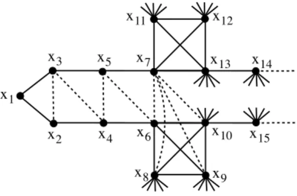
Such an example can be generalized to more complicated constraint graphs. Let us consider, for example, the graph whose a partial view is given in Fig-ure 4. We assume here that x8, x9, x10, . . . x15, . . . have a large number of
x3 x6 x7 x10 x9 x8 x5 x4 x2 x1
Figure 3: Cycle without chord on n = 10 vertices with added edges (dotted lines) by a triangulation using Min-Fill.
!" !# !$ !% !&' !&& !&" !&( !&) !&* !+ !) !* !( !&
Figure 4: A graph for which the triangulation using Min-Fill can induce clusters of arbitrarily large size.
neighboring vertices which are not represented in the figure. So, a triangu-lation using Min-Fill can find an order which is compatible with the one given by the numbering of vertices. A such order induces the clusters {x1, x2, x3}
which is connected, but also{x2, x3, x4}, {x3, x4, x5}, {x4, x5, x6}, {x4, x5, x6}
and {x5, x6, x7} which have two connected components. But such a
triangu-lation finds the cluster {x6, x7, x8, x9, x10}. Worse, we will find the cluster
{x7, x8, x9, x10, x11, x12, x13}. Of course, this example can be generalized to
find disconnected clusters of larger size.
This phenomenon is also observed for real instances, when we consider tree-decompositions of good quality. For example, the well known RLFAP instance
Scen-06 appearing in the CSP 2008 Competition3 is defined on 200 variables
and its network admit good tree-decompositions which can be found quite eas-ily (e.g. Min-Fill finds one with w+ = 20). A detailed analysis of these tree-decompositions shows that they have disconnected clusters. More generally, it turns out that about 32% of the 7,272 instances of the CSP 2008 Competition have a tree-decomposition with at least one disconnected cluster when MCS or
Min-Fill are used, what is generally the case of most tree-decomposition
meth-ods for solving CSPs. Among these instances for which MCS or Min-Fill pro-duce tree-decompositions with disconnected clusters, we can notably find most of the RLFAP or FAPP instances which are often exploited as benchmarks for decomposition methods for both decision and optimization problems. Moreover, sometimes, the percentage of disconnected clusters in one instance may be very large up to 99% and about 35% in average. For the FAPP instances, the
age is about 48% for tree-decompositions produced by Min-Fill, and a greater average using MCS. This observation will be even more striking for algorithms that find decompositions with smaller widths, as suggested by the example of the cycle without chord.
The presence of disconnected clusters in the considered tree-decomposition can have a negative impact on the practical efficiency of decomposition meth-ods which can be penalized by a large amount of time or memory to solve the instance. Firstly, the fact that a constraint network is not connected can have important consequences on the efficiency of its solving. For example, if one of its connected components has no solution, and if the solving first addresses a con-nected component that has solutions, all of them should be listed before proving the inconsistency of the whole CSP. In the case of decomposition methods, the existence of disconnected clusters is perhaps even more pernicious. In the case of Tree-Clustering, let us consider a disconnected cluster. On the one hand, the phenomenon already encountered in the case of disconnected networks may arise. But it is also possible that this cluster has solutions. All these solutions will be calculated and stored before processing another cluster. Their number can be very high as it is the product of the number of solutions of each of its connected components. Note that for some benchmarks coming from the FAPP instances, the number of connected components in one cluster can be greater than 100 while domains may have more than 100 values. However, many local solutions of this cluster may be globally incompatible, because these connected components may be linked by some constraints which appear in other clusters. Consider again the constraint graph given in Figure 4. Assume that the con-straints whose scopes are {x1, x2} and {x1, x3} are equality constraints while
all other constraints are constraints of differences. In this case, assuming that during the solving, the cluster{x7, x8, x9, x10, x11, x12, x13} will be solved before
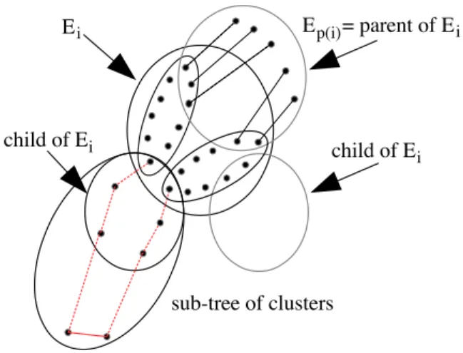
clusters containing variables located on the left in Figure 4, a large number of local solutions will be considered before finding an incompatibility one time the equality constraints will be checked. This example can be generalized by the constraint graph given in Figure 5 which shows an example of decomposition for which two connected components of a cluster Ei are connected by a sequence
of constraints that appear in the subproblem rooted in this cluster. Thus, the overall inconsistency of local solutions of Ei can only be detected when all these
clusters have been solved, during the composition of global solutions produced by Tree-Clustering in its last step. This leads Tree-Clustering to a large con-sumption of time and memory, making this approach unrealistic in practice.
To avoid this kind of phenomenon where clusters are initially solved indepen-dently, other methods were proposed like BTD. Although BTD has shown its practical advantage, unfortunately, the observed phenomenon still exists, even if it will generally be attenuated. To well understand this, let us consider a disconnected cluster Ei. We have two cases:
• if G[Ei\(Ei ∩ Ep(i))]4 is disconnected: BTD has to consistently assign
variables which are distributed in several connected components. If the subproblem rooted in Ei is trivially consistent (for instance it admits a
large number of solutions), BTD will find a solution by doing at most a few backtracks and keep on the search on the next cluster. So, in such a
4For any Y ⊆ X, the subgraph G[Y ] of G = (X, C) induced by Y is the graph (Y, C
Y)
!"""""#"$%&'()"*+"!$,-. -/0-12"*+"! -""""""""! 3456)&''"*+"/143)'&3 -/0-12"*+"!
-Figure 5: Disconnected cluster in a Tree-Decomposition. case, the non-connectivity of Ei does not entail any problem.
In contrast, if this subproblem has few solutions or none, we have a signif-icant probability that BTD passes many times from a connected compo-nent of G[Ei\(Ei∩ Ep(i))] to another when it solves this cluster. Roughly
speaking, BTD may have to explore all the consistent assignments of each connected component by interleaving eventually the variables of the differ-ent connected compondiffer-ents. Indeed, if BTD exploits filtering techniques, the assignment of a value to a variable x of Ei\(Ei∩ Ep(i)) has mainly
impact on the variables of the connected component of G[Ei\(Ei∩ Ep(i))]
which contains x. In contrast, the filtering removes no or few values from the domain of any variable in another connected component. This entails that inconsistencies are often detected later and not necessarily in Ei but
in one of its descendant cluster (as illustrated previously by Figures 4 and 5). If so, BTD may require a large amount of time or memory (due to (no)good recording) to solve the subproblem rooted in Ei, especially if the
variables have large domains. For example, this negative phenomenon has been empirically observed on some FAPP instances (e.g the fapp05-0350-10 instance) with a BTD version using MAC [42].
• if G[Ei\(Ei∩Ep(i))] is connected: since Eiis a disconnected cluster, G[Ei∩ Ep(i)] is necessarily disconnected. As the variables of the separator Ei∩ Ep(i) are already assigned, the non-connectivity of Ei does not cause any
problem.
This negative impact of disconnected clusters is compatible with empirical results reported in the literature. We have observed that sometimes, the per-centage of disconnected clusters for Min-Fill differs significantly from one for
MCS, which may explain some differences of efficiency observed in the literature
(e.g. in [24]). Indeed, even if the width is the same, decompositions computed by Min-Fill offer best results for solving than the ones obtained by MCS [24] and is considered as the best heuristic of the state of the art now [7]. Moreover, the analysis of tree-decompositions shows also that the connection between con-nected components of some clusters is frequently observed in the leaves (clusters)
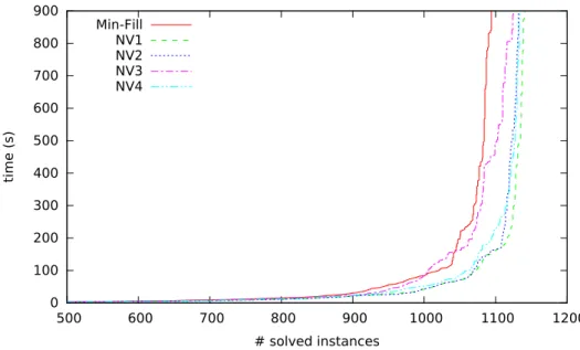
of the decomposition, further increasing more the negative effects observed. The occurrence of the negative effect of the presence of disconnected clus-ters is confirmed by the following observation. If we consider a version of BTD using a less powerful filtering than AC like Forward Checking, we see that the phenomenon is accentuated. In order to illustrate this, we analyze the solving with a particular implementation of BTD using nFC5 [3] which is the most powerful non-binary version of Forward Checking. We can thus observed that, with M in-F ill, BTD-nFC5 only solves 520 instances over the 1,668 instances with disconnected clusters we will consider in Section 6 while BTD-MAC solves 1,167 instances (see Section 6 for more details about the experimental proto-col). Moreover, if we consider the gap between the number of instances solved by BTD-MAC and BTD-nFC5 for a given decomposition method, we can note that this gap is reduced when exploiting the tree-decompositions with connected clusters introduced in the next section, namely between 485 and 499 instances against 647 with M in-F ill. This is explained by the fact that the use of a more powerful filtering as AC may lessen the phenomenon. Indeed the propagation is not limited to the neighborhood of the last assigned variable, but can reach the leaf clusters, and thus, to find some connectivity as we can see in Figure 5. Nevertheless, this level of filtering may be ineffective if one considers the example of the constraint graph given in Figure 4 with equality constraints on
{x1, x2} and {x1, x3} and constraints of differences for all other constraints.
In-deed, for this instance, the inconsistency appears on most cases, when x2 and
x3are assigned, and not when we are looking for a local solution in the cluster
{x7, x8, x9, x10, x11, x12, x13}.
To avoid this kind of phenomenon, in Section 4 we study classes of tree-decompositions for which all the clusters are connected.
3.2
The Importance of the Choice of the Root
From a practical viewpoint, generally, BTD efficiently solves CSPs having a small tree-width. However, sometimes, a bad choice for the root cluster may drastically degrade the performance of the solving. The choice of the root cluster is crucial since it impacts on the variable ordering, in particular on the choice of the first variables. Hence, in order to make a smarter choice, we have selected some instances of the CSP 2008 Competition and, for each instance, we run BTD from each cluster of its considered tree-decomposition. First, we have observed that for a given instance, the runtimes may differ from several orders of magnitude according to the chosen root cluster. For instance, for the scen11-f12 instance (which is the easiest instance of the scen11 family), BTD succeeds in proving the inconsistency for only 75 choices of root cluster among the 301 possible choices. Secondly, we have noted that solving some clusters (not necessarily the root cluster) and their corresponding subproblems is more expensive for some choice of the root cluster than for another. This is explained by the choice of the root cluster which induces some particular ordering on the clusters and the variables. In particular, since for a cluster Ei, BTD only
considers the variables of Ei\(Ei∩ Ep(i)), it does not handle the same variable
set for Ei depending on the chosen root cluster. Unfortunately, it seems to
be utopian to propose a choice for the root cluster based only on features of the instance to solve because this choice is too strongly related to the solving
efficiency. In [27], an approach has been proposed to choose a variable ordering with more freedom but its efficiency still depends on the choice of the root cluster. So, an alternative to limit the impact of the choice of the cluster is required. In Section 5, we propose a possible one consisting in exploiting restart techniques.
4
A New Parameter for Graph Decomposition
of CSPs
4.1
Bag-Connected Tree-Decomposition
The facts presented above lead us naturally to consider only tree-decompositions for which all the clusters are connected. This concept has been recently in-troduced in the context of Graph Theory [36]. It has been studied for some of its combinatorial properties. However, the algorithmic issues related to its computation have not been studied yet, neither in terms of complexity, nor to propose algorithms to find them. M¨uller provides a central theorem indicating an upper bound of Bag-Connected Tree-Width5as a function of the tree-width.
We present now the notion of Bag-Connected Tree-Decomposition, which cor-responds to tree-decomposition for which each cluster Ei is connected (i.e. the
subgraph G[Ei] of G induced by Ei is a connected graph).
Definition 3 Given a graph G = (X, C), a Bag-Connected
Tree-Decompo-sition of G is a tree-decompoTree-Decompo-sition (E, T ) of G such that for all Ei ∈ E, the subgraph G[Ei] is a connected graph. The width of a Bag-Connected Tree-Decomposition (E, T ) is equal to maxi∈I|Ei| − 1. The Bag-Connected Tree-Width wc is the minimal width over all the bag-connected tree-decompositions of G.
Given a graph G = (X, C) of tree-width w, necessarily w≤ wc. The central
theorem of [36] provides an upper bound of the Bag-Connected Tree-Width as a function of the tree-width and k which is the maximum length of its geodesic cycles6. More precisely, we have w
c ≤ w +!w+12 ".(k.w− 1) (k = 1 if G has
no cycle). This bound has been improved in [22]. Nevertheless, note that
wc=/n20 for graphs defined by cycles of length n and without chord. But if G
is a triangulated graph, w = wc.
Furthermore, the fact that w ≤ wc, independently of the complexity of
achieving a Bag-Connected Tree-Decomposition, indicates that the decomposi-tion methods based on it, necessarily appear below Tree-Decomposidecomposi-tion methods in the constraint tractability hierarchy introduced in [20]. But this remark has no real interest here because our contribution mainly concerns practical effi-ciency of such methods. Nevertheless, the difference between w and wc can
naturally have consequences on the efficiency of solving in practice. Indeed, if we consider the example of the cycle of length n given in Section 3 (a geodesic
5Note that we use the term of Bag-Connected Tree-Width rather than one of Connected
Tree-Width exploited in [36] because the term of Connected Tree-Width has been introduced before in [15] but corresponds to a quite different concept.
6A cycle is said geodesic if for any pair of vertices x and y belonging to the cycle, the
distance between x and y in the graph is equal to the length of the shortest path between x and y in the cycle.
cycle), optimal decompositions give w = 2 and wc =/n20. But, in such a case,
even if the bag-connected tree-width is arbitrarily greater than the tree-width, applying BTD based on MAC is always as effective since as soon as the first vari-able is assigned, BTD detects the inconsistency or directly finds a solution, due to the arc-consistency propagation which will be realized along the connected paths in the clusters.
The natural question now is related to the computation of optimal Bag-Connected Tree-Decompositions, that is Bag-Bag-Connected Tree-Decompositions of width wc. We show that this problem, as for Tree-Decompositions, is
NP-hard.
Theorem 1 Computing an optimal Bag-Connected Tree-Decomposition is
NP-hard.
Proof: We propose a polynomial reduction from the problem of computing an optimal decomposition to this one. Consider a graph G = (X, C) of tree-width w, the associated tree-decomposition of G being (E, T ). Now, consider the graph G! obtained by adding to G an universal vertex x, that is a vertex
which is connected to all the vertices in G. Note that from (E, T ), we can obtain a tree-decomposition for G! by adding in each cluster E
i∈ E the vertex x. It is
a bag-connected tree-decomposition since each cluster is necessarily connected (by paths containing x) and its width is w + 1. To show that this addition defines a reduction, it is sufficient to show that w is the tree-width of G iff the bag-connected tree-width wc of G! is w + 1.
(⇒) We know that at most, the width of the considered tree-decomposition
of G! is w + 1 since this tree-decomposition is connected and its width is w + 1. Thus, wc ≤ w + 1. Assume that wc ≤ w. So, there is a bag-connected
tree-decomposition of G! of width at most w. Using this tree-decomposition of G!, we can define the same tree, but deleting the vertex x, to obtain a
tree-decomposition of G of width w− 1, which contradicts the hypothesis.
(⇐) With the same kind of argument as before, we know that the tree-width
w of G is at most wc− 1. And by construction, it cannot be strictly less than wc− 1. So, it is exactly wc− 1.
Moreover, achieving G! is possible in linear time. !
We have seen that for solving CSPs, it is not necessary to find an opti-mal tree-decomposition. Also, we now propose an algorithm which computes a bag-connected tree-decomposition in polynomial time, of course without any guarantee about its optimality. The algorithm Bag-Connected-TD described below finds a bag-connected tree-decomposition of a given graph G = (X, C).
4.2
Computing a Bag-Connected Tree-Decomposition
The first step of Algorithm 2 finds a first cluster, denoted E0, which is a subset
of vertices which are connected. X! is the set of already treated vertices. It is
initialized to E0. This first step can be done easily, using an heuristic. This
heuristic may rely on any criteria as soon as it produces a connected cluster. Then, let X1, X2, . . . Xkbe the connected components of the subgraph G[X\E0]
induced by the deletion of the vertices of E0 in G. Each one of these sets is
inserted in a queue F . For each element Xi removed from the queue F , let Vi⊆ X be the set of vertices in X! which are adjacent to at least one vertex in
! " # $ % %&'(') % % *+ + , -. / 0 1 2
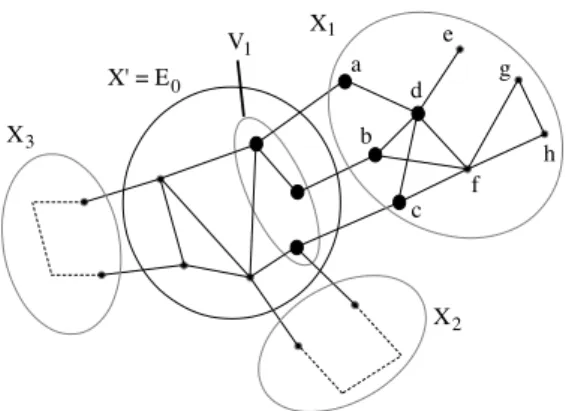
Figure 6: First pass in the loop for Bag-Connected-TD.
Xi. Note that Vi (which can be connected or not) is a separator of the graph G since the deletion of Vi in G makes G disconnected (Xi being disconnected
from the rest of G). A new cluster Ei is then initialized by this set Vi. So,
we consider the subgraph of G induced by Vi and Xi, that is G[Vi∪ Xi]. We
choose a first vertex x∈ Xi that is connected to at least one vertex of Ei (so
one vertex of Vi). This vertex is added to Ei. If G[Ei] is connected, we stop the
process because we are sure that Eiwill be a new connected cluster. Otherwise,
we continue, taking another vertex of Xi.
Figure 6 shows the computation of E1, the second cluster (after E0), at the
first pass in the loop. After the addition of vertices a, b and c, the subgraph
G[V1∪ {a, b, c}] is not connected. If the next reached vertex is d, it is added
to E1, and thus, E1 = V1∪ {a, b, c, d} is a new connected cluster, breaking the
search in G[V1∪ X1].
When this process is finished, we add the vertices of Eito X!and we compute Xi1, . . . Xiki the connected components of the subgraph G[Xi\Ei]. Each one
is then inserted in the queue F . In the example of Figure 6, two connected components will be computed,{e} and {f, g, h}. This process continues while the queue is not empty. In the example, in the right part of the graph, the algorithm will compute 3 connected clusters: {d, e}, {b, c, d, f} and {f, g, h}.
Note that line 10 is only useful when the set Vi computed at line 7 is a
previously built cluster. In such a case, the cluster Vi can be removed. Indeed,
as Vi! Ei, Vi becomes useless in the tree-decomposition.
We now establish the validity of the algorithm and we evaluate its time complexity.
Theorem 2 The algorithm Bag-Connected-TD computes the clusters of a
bag-connected tree-decomposition of a graph G.
Proof: We need only to prove lines 5-13 of the algorithm. We first prove the termination of the algorithm. At each pass through the loop, at least one vertex will be added to the set X! and this vertex will not appear later in a new
element of the queue because they are defined by the connected components of
G[Xi\Ei], a subgraph that contains strictly fewer vertices than was contained
in Xi. So, after a finite number of steps, the set Xi\Ei will be an empty set,
Algorithm 2: Bag-Connected-T D
Input: A graph G = (X, C)
Output: A set of clusters E0, . . . Eqof a bag-connected tree-decomposition of G 1 Choose a first connected cluster E0in G
2 X!← E0
3 Let X1, . . . Xkbe the connected components of G[X\E0]
4 F← {X1, . . . Xk}
5 while F%= ∅ do /* find a new clusterEi */ 6 Remove Xifrom F
7 Let Vi⊆ X!be the neighborhood of Xiin G 8 Ei← Vi
9 Search in G[Vi∪ Xi] starting from Vi∪ {x} with x ∈ Xi. Each time a new vertex x is
found, it is added to Ei. The process stops once the subgraph G[Ei] is connected
10 if Vibelongs to the set of clusters already found then Delete the cluster Vi(because
Vi! Ei)
11 X!← X!∪ Ei
12 Let Xi1, Xi2, . . . Xiki be the connected components of G[Xi\Ei]
13 F← F ∪ {Xi1, Xi2, . . . Xiki}
We now show that the set of clusters E0, E1, . . . Eq induces a bag-connected
tree-decomposition. By construction each new cluster is connected. So, we have only to prove that they induce a tree-decomposition. We prove this by induction on the added clusters, showing that all these added clusters will induce a tree-decomposition of the graph G(X!).
Initially, the first cluster E0 induces a tree-decomposition of the graph
G[E0] = G[X!].
For the induction, our hypothesis is that the set of already added clusters
E0, E1, . . . Ei−1induces a tree-decomposition of the graph G[E0∪E1∪· · ·∪Ei−1].
Consider now the addition of Ei. We show that by construction, E0, E1, . . . Ei−1
and Ei induces a tree-decomposition of the graph G[X!] by showing that the
three conditions (i), (ii) and (iii) of the definition of tree-decompositions are satisfied.
(i) Each new vertex added in X! belongs to Ei
(ii) Each new edge in G[X!] is inside the cluster Ei.
(iii) We can consider two different cases for a vertex x∈ Ei, knowing that for
other vertices, the property is already satisfied by the induction hypothesis: (a) x∈ Ei\Vi: in this case, x does not appear in another cluster than Ei
and then, the property holds.
(b) x ∈ Vi: in this case, by the induction hypothesis, the property was
already verified.
Finally, it is easy to see that if line 10 is applied, we obtain a tree-decomposition of the graph G[X!]. !
Theorem 3 The time complexity of the algorithm Bag-Connected-TD is O(n(n+
e)).
Proof: Lines 1-4 are feasible in linear time, that is O(n + m), since the cost of computing the connected components of G[X\E0] is bounded by O(n + m).
to get a more relevant first cluster, but at most in O(n(n + m)) in order not to exceed the time complexity of the most expensive step of the algorithm. We analyze now the cost of the loop (line 5). Firstly, note that there are less than n insertions in the queue F . Now, we analyze the cost of each treatment associated to the addition of a new cluster, and we give for each one, its global complexity.
• Line 6: obtaining the first element Xi of F is bounded by O(n), thus
globally O(n2).
• Line 7: obtaining the neighborhood Vi ⊆ X! of Xi in G is bounded by
O(n + m), thus globally by O(n(n + m)).
• Line 8: this step is feasible in O(n), thus globally O(n2).
• Line 9: the cost of the search in G[Vi∪ Xi] starting with vertices of Vi
and x∈ Xi is bounded by O(n + m). Since the while loop runs at most n times, the global cost of the search in these subgraphs is bounded by
O(n(n + m)). Moreover, for each new added vertex x, the connectivity of
G[Ei] is tested with an additional cost bounded by O(n + m). Note since
such a vertex is added at most one time, globally, the cost of this test is bounded by O(n(n + m)). So, the cost of line 9 is globally bounded by O(n(n + m)).
• Line 10: using an efficient data structure, this step can be realized in O(n),
thus globally O(n2).
• Line 11: the union is feasible in O(n), thus globally O(n2) since there are
at most n iterations.
• Line 12: the cost of finding the connected components of G[Xi\Ei] is
bounded by O(n + m). So, globally, the cost of this step is O(n(n + m)).
• Line 13: the insertion of a set Xij in F is feasible in O(n), thus globally
O(n2) since there are less than n insertions in F .
Finally, the time complexity of the algorithm Bag-Connected-TD is O(n(n+m)).
!
From a practical viewpoint, it can be assumed that the choice of the first cluster E0 can be crucial for the quality of the decomposition which is being
computed. Similarly, the choice of vertex x, selected in line 9 may be of con-siderable importance. For these two choices, heuristics can of course be used. This is discussed in Section 6. However, a particular choice of these heuristics makes it possible, without any change of the complexity, to compute optimal tree-decompositions for the case of triangulated graphs. Assume that the first cluster E0 is a maximal clique. This can be done efficiently using a greedy
approach. Now, for the choice of the vertex x in line 9, we consider the vertex which has the maximum number of neighbors in the set Vi. As in a triangulated
graph, all the clusters of an optimal tree-decomposition are cliques, necessar-ily, Vi being a clique, x will be connected to all the vertices of Vi and thus, Ei will be a clique. Progressively, each maximal clique will be found and the
tree-decomposition will be optimal. Line 10 will be used for the case of maximal cliques including more than one vertex x of a new connected component. In any
case, the practical interest of this type of decomposition is based on both the efficiency of its computation, but also on the significance which it may have for solving CSPs. This is discussed in Section 6.
5
Exploiting Restarts within BTD
In this section, we explain how BTD can safely exploit restarts.
It is well known that any method exploiting restart techniques must as much as possible avoid exploring the same part of the search space several times and that randomization and learning are two possible ways to reach this aim [33]. Regarding the learning, BTD already exploits structural (no)goods. However, depending on when the restart occurs, we have no warranty that a structural (no)good has been recorded yet. Hence, another form of learning is required to ensure a good practical efficiency. Here, we consider the reduced nld-nogoods [34].
The use of learning in BTD may endanger its correctness as soon as we add to the initial problem a constraint whose scope is not included in a cluster. So recording reduced nld-nogoods in a global constraint involving all the variables like proposed in [34] is impossible. However, by exploiting the features of a compatible variable ordering, Property 2 shows that this global constraint can be safely decomposed in a global constraint per cluster Ei.
Proposition 2 Let Σ = &δ1, . . . , δk' be the sequence of decisions taking along the branch of the search tree when solving a CSP P by exploiting a tree-decompo-sition (E, T ) and a compatible variable ordering. Let Σ[Ei] be the subsequence built by considering only the decisions of Σ involving the variables of Ei. For any prefix subsequence Σ!
Ei =&δi1, . . . , δi!' of Σ[Ei] s.t. δi! is a negative decision,
and every variable in Ei ∩ Ep(i) appears in a decision in P os(Σ!Ei), the set
P os(Σ!Ei)∪ {¬δi!} is a reduced nld-nogood of P .
Proof: Let PEi be the subproblem induced by the variables of Desc(Ei) and
∆Ei the set of the decisions of P os(ΣEi) related to the variables of Ei∩ Ep(i).
As Ei∩Ep(i)is a separator of the constraint graph, PEi|∆Ei is independent from
the remaining part of the problem P . Let us consider Σ[Ei] the maximal
subse-quence of Σ which only contains decisions involving variables of Ei. According
to Proposition 1 applied to Σ[Ei] and PEi|∆Ei, P os(Σ!Ei)∪ {¬δi!} is necessarily
a reduced nld-nogood. !
It ensues that we can bound the size of produced nogoods and compare them with those produced by Proposition 1:
Corollary 1 Given a tree-decomposition of width w+, the size of reduced
nld-nogood produced by proposition 2 is at most w++ 1.
Corollary 2 Under the same assumptions as Proposition 2, for any reduced
nld-nogood ∆ produced by Proposition 1, there is at least one reduced nld-nogood
∆! produced by Proposition 2 s.t. ∆! ⊆ ∆.
Proof: Let Σ! =&δ1, . . . , δ!' be a subsequence of Σ s.t. δ!is a negative decision.
From Proposition 1, it follows that ∆ = P os(Σ!)∪{¬δ!} is a reduced nld-nogood.