Region Array SSA

HAL Id: hal-03106226

https://hal.archives-ouvertes.fr/hal-03106226

Submitted on 11 Jan 2021

HAL is a multi-disciplinary open access

archive for the deposit and dissemination of

sci-entific research documents, whether they are

pub-lished or not. The documents may come from

teaching and research institutions in France or

abroad, or from public or private research centers.

L’archive ouverte pluridisciplinaire HAL, est

destinée au dépôt et à la diffusion de documents

scientifiques de niveau recherche, publiés ou non,

émanant des établissements d’enseignement et de

recherche français ou étrangers, des laboratoires

publics ou privés.

Region Array SSA

Silvius Rus, Guobin He, Christophe Alias, Lawrence Rauchwerger

To cite this version:

Silvius Rus, Guobin He, Christophe Alias, Lawrence Rauchwerger. Region Array SSA. ACM/IEEE

International Conference on Parallel Architectures and Compilation Techniques (PACT’06), Sep 2006,

Seattle, United States. �hal-03106226�

Region Array SSA

Silvius Rus

Texas A&M University

Guobin He

Texas A&M University

Christophe Alias

ENS Lyon

Lawrence Rauchwerger

Texas A&M University

ABSTRACT

Static Single Assignment (SSA) has become the intermedi-ate program representation of choice in most modern com-pilers because it enables efficient data flow analysis of scalars and thus leads to better scalar optimizations. Unfortunately not much progress has been achieved in applying the same techniques to array data flow analysis, a very important and potentially powerful technology. In this paper we propose to improve the applicability of previous efforts in array SSA through the use of a symbolic memory access descriptor that can aggregate the accesses to the elements of an ar-ray over large, interprocedural program contexts. We then show the power of our new representation by using it to implement a basic data flow algorithm, reaching definitions. Finally we apply this analysis to array constant propagation and array privatization and show performance improvement (speedups) for benchmark codes.

1.

INTRODUCTION

Important compiler optimization or enabling transforma-tions such as constant propagation, loop invariant motion, expansion/privatization depend on the power of data flow analysis. The Static Single Assignment (SSA) [10] program representation has been widely used to explicitly represent the flow between definitions and uses in a program.

SSA relies on assigning each definition a unique name and ensuring that any use may be reached by a single definition. The corresponding unique name appears at the use site and offers a direct link from the use to its corresponding and unique definition. When multiple control flow edges carry-ing different definitions meet before a use, a special φ node ∗_{This research supported in part by NSF Grants} EIA-0103742, ACR-0081510, ACR-0113971, CCR-0113974, ACI-0326350, and by the DOE.

†_{Parasol Lab, Department of Computer Science, Texas} A&M University, {silviusr,guobinh,rwerger}@cs.tamu.edu. ‡_{Laboratoire de l’Informatique du Parall´elism, ENS Lyon,} Christophe.Alias@ens-lyon.fr

Permission to make digital or hard copies of all or part of this work for personal or classroom use is granted without fee provided that copies are not made or distributed for profit or commercial advantage and that copies bear this notice and the full citation on the first page. To copy otherwise, to republish, to post on servers or to redistribute to lists, requires prior specific permission and/or a fee.

PACT’06, September 16–20, 2006, Seattle, Washington, USA.

Copyright 2006 ACM 1-59593-264-X/06/0009 ...$5.00. x = 5 x = 7 . . . = x (a) x1 = 5 x2 = 7 . . . = x2 (b) A(3) = 5 A(4) = 7 . . . = A(3) (c) A1(3) = 5 A2(4) = 7 . . . = A2(3) (d) Figure 1: (a) Scalar code, (b) scalar SSA form, (c) array code and (d) improper use of scalar SSA form for arrays.

is inserted at the merge point. Merge nodes are the only statements allowed to be reached directly by multiple defi-nitions.

Classic SSA is limited to scalar variables and ignores con-trol dependence relations. Gated SSA [1] introduced concon-trol dependence information in the φ nodes. This helps select-ing, for a conditional use, its precise definition point when the condition of the definition is implied by that of the use [27]. The first extensions to array variables ignored array indices and treated each array definition as possibly killing all previous definitions. This approach was very limited in functionality. Array SSA was proposed by [16, 24] to match definitions and uses of partial array regions. However, their approach of representing data flow relations between indi-vidual array elements makes it difficult to complete the data flow analysis at compile time and requires potentially high overhead run-time evaluation. Section 6 presents a detailed comparison of our approach against previous related work.

We propose an Array SSA representation of the program that accurately represents the use-def relations between ar-ray regions and accounts for control dependence relations. We use the USR symbolic representation of array regions [23] which can represent uniformly memory location sets in a compact way for both static and dynamic analysis tech-niques. We present a reaching definition algorithm based on Array SSA that distinguishes between array subregions and is control accurate. The algorithm is used to implement array constant propagation and array privatization for au-tomatic parallelization, for which we present whole appli-cation improvement results. Although the Array SSA form that we present in this paper only applies to structured pro-grams that contain no recursive calls, it can be generalized to any programs with an acyclic Control Dependence Graph (except for self-loops).

2.

REGION ARRAY SSA FORM

Static Single Assignment (SSA) is a program representa-tion that presents the flow of values explicitly. In Fig. 1(a), the compiler must analyze the control flow graph in order to

Author version

Do i =1 ,3 A1( i )=0 Enddo Do i =1 ,3 A2( i +3)=1 EndDo @A3= M AX(@A1, @A2) (a) Array SSA @A3= [(A1, 1), (A1, 2), (A1, 3), (A2, 1), (A2, 2), (A2, 3)] S i m p l i f i e d v e r s i o n @A3= [A1, A1, A1, A2, A2, A2] Aggregated a r r a y r e g i o n s A3← A1= [1 : 3] A3← A2= [4 : 6] (b)

Figure 2: (a) Sample code in Array SSA form (not all gates shown for simplicity). (b) Array SSA forms: (top) as proposed by [16], (center) with reduced accuracy and (bottom) using aggregated array regions.

decide which of the two values, 5 or 7, will be used in the last statement. By numbering each static definition and match-ing them with the correspondmatch-ing uses, the use-def chains become explicit. In Fig. 1(b) it is clear that the value used is x2 (7) and not x1 (5).

Unfortunately, such a simple construction cannot be built for arrays the same way as for scalars. Fig. 1(d) shows a failed attempt to apply the same reasoning to the code in Fig. 1(c). Based on SSA numbers, we would draw the con-clusion that the value used in the last statement is that defined by A2, which would be wrong. The fundamental reason why we cannot extend scalar SSA form to arrays di-rectly is that an array definition generally does not kill all previous definitions to the same array variable, unlike in the case of scalar variables. In Fig. 1(c), the second definition does not kill the first one. In order to represent the flow of values stored in arrays, the SSA representation must ac-count for individual array elements rather than treating the whole array as a scalar.

Element-wise Array SSA was proposed as a solution by [24]. Essentially, for every array there is a corresponding @ array, which stores, at every program point and for every array element, the location of the corresponding reaching definition under the form of an iteration vector. The com-putation of @ arrays consists of lexicografic MAX operations on iteration vectors. Although there are methods to reduce the number of MAX operation for certain cases, in general they cannot be eliminated. This led to limited applicability for compile-time analysis and potentially high overhead for derived run-time analysis, because the MAX operation must be performed for each array element.

We propose a new Region Array SSA (RA SSA) repre-sentation. Rather than storing the exact iteration vector of the reaching definition for each array location, we just store the SSA name of the reaching definition. Although our rep-resentation is not as precise as [24], that did not affect the success of our associated optimization techniques. This sim-plification allowed us to employ a different representation of @ arrays as aggregated array regions. Fig. 2 depicts the relation between element-wise Array SSA and our Region Array SSA. Rather than storing for each array element its reaching definition, we store, for each use-def relation such as A3 ← A1, the whole array region on which values defined at A1 reach A3.

We use the USR [23] representation for array regions, which can represent uniformly arbitrarily complex regions. Moreover, when an analysis based on USRs cannot reach a static decision, the analysis can be continued at run time with minimal necessary overhead. For instance, in the ex-ample in Fig. 2, let us assume that the loop bounds were not known at compile time. In that case the MAX oper-ation could not be performed statically. Its run time as proposed by [24] would require O(n) time, where n is the dimension of the array. Using Region Array SSA, the region corresponding to A3 ← A1can be computed at run time in O(1) time, thus independent of the array size. Our resulting Region Array SSA representation has two main advantages over [16]:

• We can analyze many complex patterns at compile time using symbolic array region analysis (essentially symbolic set operations), whereas the previous Array SSA represen-tation often fails to compute element-wise MAX operations symbolically (for the complex cases).

• When a static optimization decision cannot be reached, we can extract significantly less expensive run time tests based on partial aggregation of array regions.

We will now present the USR representation for array re-gions, describe the structure of Region Array SSA, and then illustrate its use in an algorithm that computes reaching definitions for arrays.

2.1

Array Region Representation: the USR

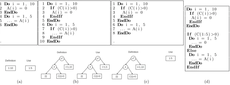
In the example in Fig. 3(a), we can safely propagate con-stant value 0 from the definition at site 2 to the use at site 5 because the array region used, [1:5], is included in the array region defined above, [1:10]. In the example in Fig. 3(b), we cannot represent the array regions as intervals because the memory references are guarded by an array of conditionals. However, we can represent the array regions as expressions on intervals, in which the operators represent predication (#) and expansion across an iteration space (⊗∪_{). This} symbolic representation allows us to compare the defined and used regions even though their shapes are not linear. In the example in Fig. 3(c), a static decision cannot be made. The needed values of the predicate array C(:) may only be known at run time. We can still perform constant propaga-tion on array A optimistically and validate the transforma-tion dynamically, in the presence of the actual values of the predicate array. Although the profitability of such a trans-formation in this particular example is debatable due to the possibly high cost of checking the values of C(:) at run time, in many cases such costs can be reduced by partial aggrega-tion and amortized through hoisting and memoizaaggrega-tion.

The Uniform Set of References (USR) previously intro-duced in [23]1formalizes the expressions on intervals shown in Fig. 3. It is a general, symbolic and analytical repre-sentation for memory reference sets in a program. It can represent the aggregation of scalar and array memory refer-ences at any hierarchical level (on the loop and subprogram call graph) in a program. It can represent the control flow (predicates), inter-procedural issues (call sites, array reshap-ing, type overlaps) and recurrences. The simplest form of a USR is the Linear Memory Access Descriptor (LMAD) [20], a symbolic representation of memory reference sets accessed through linear index functions. It may have multiple dimen-1_{USRs were presented there under the name of RT LMAD} because they were used mostly to produce run time tests.

1 Do i = 1 , 10 2 A( i ) = 0 3 EndDo 4 Do i = 1 , 5 5 . . . = A( i ) 6 EndDo . 1 Do i = 1 , 10 2 I f (C( i ) >0) 3 A( i ) = 0 4 EndIf 5 EndDo 6 Do i = 1 , 5 7 I f (C( i ) >0) 8 . . . = A( i ) 9 EndIf 10 EndDo 1 Do i = 1 , 10 2 I f (C( i ) >0) 3 A( i ) = 0 4 EndIf 5 EndDo 6 Do i = 1 , 5 7 . . . = A( i ) 8 EndDo . 1:10 1:5 Definition Use x U i=1,10 # {i} C(i)>0 xU i=1,5 # {i} C(i)>0 Definition Use xU i=1,10 # {i} C(i)>0 1:5 Definition Use Do i = 1 , 10 I f (C( i ) >0) A( i ) = 0 EndIf EndDo I f (C( 1 : 5 ) > 0 ) Do i = 1 , 5 . . . = 0 EndDo Else Do i = 1 , 5 . . . = A( i ) EndDo EndIf (a) (b) (c) (d)

Figure 3: Constant propagation scenarios: (a) symbolically comparable linear reference pattern, (b) symbolically comparable nonlinear reference pattern, (c) nonlinear reference pattern that require a run time test and (d) dynamic constant propagation code for case (c).

sions, and all its components may be symbolic expressions. Throughout this paper we will use the simpler interval nota-tion for unit-stride single dimensional LMADs. For the loop in Fig. 3(a), the array subregion defined by the first loop can be represented as an LMAD, [1:10], and the array subregion used in the second loop can also be represented as another LMAD, [1:5].

The USR is stored as an abstract syntax tree with respect to the language presented in Fig. 4 and can be thought of as symbolic expressions on sets of memory locations. When memory references are expressed as linear functions, USRs consist of a single leaf, i.e., a list of LMADs. When the analysis process encounters a nonlinear reference pattern or when it performs an operation (such as set difference) whose result cannot be represented as a list of LMADs, we add internal nodes that record accurately the operations that could not be performed.

In the examples in Fig. 3(b,c), memory references are predicated by an array of conditions. This nonlinear ref-erence pattern cannot be represented as an LMAD, so it is expressed as a nontrivial USR. Although nothing is known about the predicates, the USR representation allows us to compare the definition and use sets symbolically in case (b). In case (c) a static decision cannot be made. However, us-ing USRs we can formulate efficient run time tests that will guarantee the legality of the constant propagation transfor-mation at run time. [23] showed how to extract efficient run time tests from identities of type S = ∅, where S is a USR. By setting S = used − def ined, we can extract conditions that guarantee the safety of the optimistic constant propa-gation (Fig. 3(d)). Additionally, constant propapropa-gation may enable other more profitable transformations such as auto-matic parallelization by simplifying the control flow and the memory reference pattern.

Most examples in this paper only present single-indexed arrays accessed using a unit stride solely for the simplic-ity of the presentation. The USRs can represent any mem-ory reference pattern produced by multidimensional arrays accessed over arbitrary large loop nests spanning multiple subroutines. Strides can be arbitrary symbolic expressions.

Σ = {∩, ∪, −, (, ), #, ⊗∪_,⊗∩_{, ⊲⊳,}

LM ADs, Gate, Recurrence, CallSite} N= {U SR}, S= U SR P = {U SR → LM ADs|(U SR) U SR→ U SR ∩ U SR U SR→ U SR ∪ U SR U SR→ U SR − U SR U SR→ Gate#U SR U SR→ ⊗∪ RecurrenceU SR U SR→ ⊗∩ RecurrenceU SR U SR→ U SR ⊲⊳ CallSite}

Figure 4: USR formal definition. ∩, ∪, − are ele-mentary set operations: intersection, union, difference. Gate#U SR represents reference set U SR predicated by condition Gate. ⊗∪

i=1,nU SR(i) represents the union of ref-erence sets U SR(i) across the iteration space i = 1, n. U SR(f ormals) ⊲⊳ Call Site represents the image of the generic reference set U SR(f ormals) instantiated at a par-ticular call site.

USRs also contain control dependence information. The only restriction is that the program must be structured.

2.2

Array SSA Definition and Construction

2.2.1

Region Array SSA Nodes

In scalar SSA, pseudo statements φ are inserted at con-trol flow merge points. These pseudo statements show which scalar definitions are combined. [1] refines the SSA pseudo statements in three categories, depending on the type of merge point: γ for merging two forward control flow edges, µ for merging a loop-back arc with the incoming edge at the loop header, and η to account for the possibility of zero-trip loops. The array SSA form proposed in [24] presents the need for additional φ nodes after each assignment that does not kill the whole array. These extensions, while necessary, are not sufficient to represent array data flow efficiently be-cause they do not represent array indices.

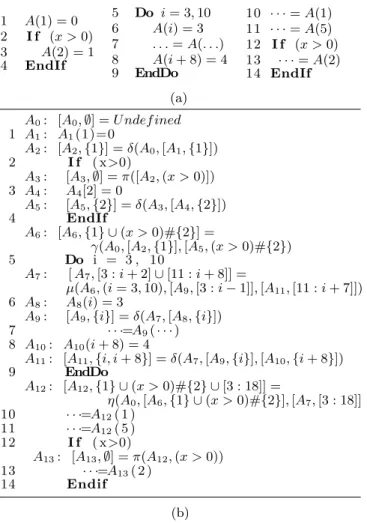
nec-1 A(1) = 0 2 I f (x > 0) 3 A(2) = 1 4 EndIf 5 Do i = 3, 10 6 A(i) = 3 7 . . . = A(. . .) 8 A(i + 8) = 4 9 EndDo 10 · · · = A(1) 11 · · · = A(5) 12 I f (x > 0) 13 · · · = A(2) 14 EndIf (a) A0: [A0, ∅] = U ndef ined 1 A1: A1(1)=0 A2: [A2, {1}] = δ(A0, [A1, {1}]) 2 I f ( x>0) A3: [A3, ∅] = π([A2, (x > 0)]) 3 A4: A4[2] = 0 A5: [A5, {2}] = δ(A3, [A4, {2}]) 4 EndIf A6: [A6, {1} ∪ (x > 0)#{2}] = γ(A0, [A2, {1}], [A5, (x > 0)#{2}) 5 Do i = 3 , 10 A7: [ A7, [3 : i + 2] ∪ [11 : i + 8]] = µ(A6, (i = 3, 10), [A9, [3 : i − 1]], [A11, [11 : i + 7]]) 6 A8: A8(i) = 3

A9: [A9, {i}] = δ(A7, [A8, {i}]) 7 · · ·=A9( · · · ) 8 A10: A10(i + 8) = 4

A11: [A11, {i, i + 8}] = δ(A7, [A9, {i}], [A10, {i + 8}])

9 EndDo A12: [A12, {1} ∪ (x > 0)#{2} ∪ [3 : 18]] = η(A0, [A6, {1} ∪ (x > 0)#{2}], [A7, [3 : 18]] 10 · · ·=A12( 1 ) 11 · · ·=A12( 5 ) 12 I f ( x>0) A13: [A13, ∅] = π(A12, (x > 0)) 13 · · ·=A13( 2 ) 14 Endif (b)

Figure 5: (a) Sample code and (b) Array SSA form

essary to incorporate array region information into the rep-resentation. Region Array SSA gates differ from those in scalar SSA in that they represent, at each merge point, the array subregion (as a USR) corresponding to every φ func-tion argument. [An,ℜn] = φ(A0,[A1,ℜn1], [A2,ℜn2], . . . , [Am,ℜnm]) (1) whereℜn= m [ k=1 ℜn kandℜ n i ∩ ℜnj = ∅, (2) ∀ 1 ≤ i, j ≤ m, i 6= j

Equation 1 shows the general form of a φ node in Region Array SSA. ℜn

k is the array region (as USR) that carries values from definition Ak to the site of the φ node. Since ℜn

k are mutually disjoint, they provide a basic way to find the definition site for the values stored within a specific array region at a particular program context. Given a set ℜU se(An)

of memory locations read right after An, equation 1 tells us that ℜU se(An)∩ ℜ

n

k was defined by Ak. The free term A0 is used to report locations undefined within the program block that contains the φ node. Let us note that two array regions can be disjoint because they represent different locations but also because they are controlled by contradictory predicates. Essentially, our φ nodes translate basic data flow relations to USR comparisons. These USR comparisons can

• be performed symbolically at compile time in most prac-tical cases, and

• be solved at run time with minimal necessary overhead, based on USR partial aggregation capabilities.

Our node placement scheme is essentially the same as in [24]. In addition to φ nodes at control flow merge points, we add a φ node after each array definition. These new nodes are named δ. They merge the effect of the immediately previous definition with that of all other previous definitions. Each node corresponds to a structured block of code. In the example in Fig. 5, A2 corresponds to statement 1, A6 to statements 1 to 4, A11 to statements 6 to 8, and A12 to statements 1 to 9. In general, a δ node corresponds to the maximal structured block that ends with the previous statement.

2.2.2

Abstraction of Partial Kills:

Nodes

In the example in Fig. 5, the array use A(1) at statement 10 could only have been defined at statement 1. Between statement 1 and statement 10 there are two blocks, an If and a Do. We would like to have a mechanism that could quickly tell us not to search for a reaching definition in any of those blocks. We need SSA nodes that can summarize the array definitions in these two blocks. Such summary nodes could tell us that the range of locations defined from statement 2 to statement 9 does not include A(1).

The function of a δ node is to aggregate the effect of dis-joint structured blocks of code. 2 _{Fig. 6(a) shows the way we} build δ gates for straight line code. Since the USR represen-tation contains built-in predication, expansion by a recur-rence space and translation across subprogram boundaries, the δ functions become a powerful mechanism for computing accurate use-def relations.

Returning to our example, the exact reaching definition of the use at line 10 can be found by following the use-def chain {A12, A6, A2, A1}. A use of A12(20) can be classified as undefined using a single USR intersection, {A12, A0}.

2.2.3

Abstraction of Loops:

Nodes

The semantics of µ for Array SSA is different than those for scalar SSA. Any scalar assignment kills all previous ones (from a different statement or previous iteration). In Array SSA, different locations in an array may be defined by var-ious statements in varvar-ious iterations, and still be visible at the end of the loop. In the code in Fig. 5(a), Array A is used at statement 7 in a loop. In case we are only interested in its reaching definitions from within the same iteration of the loop (as is the case in array privatization), we can apply the same reasoning as above, and use the δ gates in the loop body. However, if we are interested in all the reaching def-initions from previous iterations as well as from before the loop, we need additional information. The µ node serves this purpose.

[An, ℜn] = µ(A0, (i = 1, p), [A1, ℜn1], . . . , [Am, ℜnm]) (3) The arguments in the µ statement at each loop header are all the δ definitions within the loop that are at the immediately inner block nesting level (Fig. 6(c)), and in the order in which they appear in the loop body. Sets ℜn

k are functions of the loop index i. They represent the sets of memory 2_{A δ function at the end of a Do block is written as η, and} at the end of an If block as γ to preserve the syntax of the conventional GSA form. A δ function after a subroutine call is marked as θ, and summarizes the effect of the subroutine call on the array.

locations defined in some iteration j < i by definition Ak and not killed before reaching the beginning of iteration i. For any array element defined by Ak in some iteration j < i, in order to reach iteration i, it must not be killed by other definitions to the same element, which occur from that point on until the beginning of iteration i. We must thus subtract the regions defined in iteration j after definition Ak: Kills(j), as well as all the regions defined in the subsequent iterations j + 1, ..., i − 1: Killa(l). ℜn k(i) = ∪ O j=1,i−1 2 4ℜk(j) − 0 @Kills(j) ∪ ∪ O l=j+1,i−1 Killa(l) 1 A 3 5 (4) where Kills= m [ h=k+1 ℜh, and Killa= m [ h=1 ℜh

This representation gives us powerful closed forms for array region definitions across the loop. We avoid fixed point iter-ation methods by hiding the complexity of computing closed forms in USR operations. The USR simplification process will attempt to reduce these expressions to LMADs. How-ever, even when that is not possible, the USR can be used in symbolic comparisons (as in Fig. 3(b)), or to generate ef-ficient run-time assertions (as in Fig. 3(c)) that can be used for run-time optimization and speculative execution.

The reaching definition for the array use A12(5) at state-ment 11 (Fig. 5(b)) is found inside the loop using δ gates. We use the µ gate to narrow down the block that defined A(5). We intersect the use region {5} with ℜ79(i = 11) = [3 : 10], and ℜ7

11(i = 11) = [11 : 18]. We substituted i ← 11, because the use happens after the last iteration. The use-def chain is {A12, A7, A9}.

2.2.4

Abstraction of Control:

Nodes

The control dependence predicates corresponding to array definitions are embedded in USRs as seen in the γ gate at the definition site of A6 in Fig. 5. The remainder of this section presents an extension to classic SSA which represents explicitly the control predicates of array uses.

Array element A13(2) is used conditionally at statement 13. Based on its range, it could have been defined only by statement 3. In order to prove that it was defined at state-ment 3, we need to have a way to associate the predicate of the use with the predicate of the definition. We create fake definition nodes π to guard the entry to control de-pendence regions associated with Then and Else branches: [An, ∅] = π(A0, cond). This type of gate does not have a correspondent in classic scalar SSA, but in the Program De-pendence Web [1]. Their advantage is that they lead to more accurate use-def chains. Their disadvantage is that they create a new SSA name in a context that may con-tain no array definitions. Such a fake definition A13 placed between statement 12 and 13 will force the reaching defini-tion search to collect the condidefini-tional x > 1 on its way to the possible reaching definition at line 2. This conditional is crucial when the search reaches the γ statement that defines A6, which contains the same condition. The use-def chain is {A13, A12, A6, A5, A4}.

2.2.5

Array SSA Construction

Fig. 6 presents the way we create δ, η, γ, µ, and π gates for various program constructs. The associated array regions

1 A(R1) = . . . 2 A(R2) = . . . n A(Rn) = . . . [A0, ∅] = U ndef ined A1(R1) = . . . [A2, R1] = δ(A0, [A1, R1]) A3(R2) = . . . [A4, R1∪ R2] = δ(A0, [A2, R1− R2], [A3, R2]) A2n−1(Rn) = . . . [A2n,Sn_i=1Ri] = δ(A0, [A2n−2,Sn−1_i=1 Ri− Rn], [A2n−1, Rn])

(a) Straight line code.

1 A(Rx) = . . . 2 I f ( cond ) 3 A(Ry) = . . . 4 EndIf [A0, ∅] = U ndef ined A1(Rx) = . . . [A2, Rx] = δ(A0, [A1, Rx]) I f ( cond ) [A3, ∅] = π(A2, cond) A4(Ry) = . . . [A5, Ry] = δ(A3, [A4, Ry]) EndIf [A6, Rx∪ cond#Ry] =

γ(A0, [A2, Rx− cond#Ry], [A5, cond#Ry])

(b) If block. 1 Do i =1 ,n 2 A(Rx(i)) = . . . 3 A(Ry(i)) = . . . 4 EndDo [A0, ∅] = U ndef ined Do i =1 ,n [A5, ℜ52(i) ∪ ℜ54(i)] =

µ(A0, (i = 1, n), [A2, ℜ52(i)], [A4, ℜ54(i)]) A1(Rx(i)) = . . .

[A2, Rx(i)] = δ(A5, [A1, Rx]) A3(Ry(i)) = . . .

[A4, Rx(i) ∪ Ry(i)] =

δ(A5, [A2, Rx(i) − Ry(i)], [A3, Ry(i)]) EndDo

[A6, ⊗∪i=1,n(ℜ52(i) ∪ ℜ54(i))] =

η([A0, ∅], [A5, ⊗∪i=1,n(ℜ52(i) ∪ ℜ54(i))])

(c) Do block. ℜ5

k(i) = definitions from Aknot killed upon entry to iteration i (Equation 4).

Figure 6: Region Array SSA transformation: original code on the left, Region Array SSA code on the right.

are built in a bottom-up traversal of the Control Depen-dence Graph intraprocedurally, and the Call Graph inter-procedurally. At each block level (loop body, then branch, else branch, subprogram body), we process sub-blocks in program order.

2.2.6

Complexity

The number of φ nodes is O(|E(CF G)| ∗ V ariable Count because every statement (CFG node) could modify all the variables. [23] showed that the number of USR nodes added by each operation (union, intersection, etc) is O(1), and that each USR node consumes O(1) memory. Since the number of USR operations to build any φ node is also O(1), the space complexity is thus O(|E(CF G)| ∗ V ariable count.

USR construction optimizations such as symbolic aggre-gation push the time of each operation to O(|V (CF G)|) in the worst case, though we have observed in practice an amor-tized O(1). The total compilation time ranges from seconds on a 200 lines code to minutes on a 5000 lines code, using a Pentium IV 2.8GHz PC.

2.3

Reaching Definitions

Algorithm S e a r c h ( Au, ℜuse, GivenBlock ) I f Au6∈ GivenBlock o r ℜuse= ∅ Then Return Switch def inition site(Au)

Case original statement : ℜRD

u = ℜu∩ ℜuse

Case δ , γ , η , θ : [Au, ℜu] = φ(A0, [A1, ℜu1], . . .) ForEach [Ak, ℜuk]

Call S e a r c h ( Ak, ℜuse∩ ℜuk, GivenBlock ) Call S e a r c h ( A0, ℜuse− ℜn, GivenBlock ) Case µ : [Au, ℜu(i)] = µ(A0, (i = 1, p), [A1, ℜu1(i)], . . .)

ForEach [Ak, ℜuk(i)]

Call S e a r c h ( Ak, ℜuse(i) ∩ ℜuk(i) , Block(Ak) ) Call S e a r c h ( A0, ⊗∪i=1,p(ℜuse(i) − ℜu(i)) , GivenBlock ) Case π(A0, cond)

Call S e a r c h ( A0, cond#ℜuse, GivenBlock ) EndIf

Figure 7: Recursive algorithm to find reaching defini-tions. Au is an SSA name and ℜuse is an array region. Array regions ℜ are represented as USRs. They are built using USR operations such as ∩, −, #, ⊗∪_.

Finding the reaching definitions for a given use is required to implement a number of optimizations: constant propaga-tion, array privatization etc. We present here a general algo-rithm based on Array SSA that finds, for a given SSA name and array region, all the reaching definitions and the corre-sponding subregions. These subregions can then be used to implement particular optimizations such as constant prop-agation. Any such optimization can be performed either at compile time, when associated USR comparison can be solved symbolically, or at run-time, when USR comparisons depend on input values.

For each array use ℜU se(Au)of an SSA name Au, and for a

given block, we want to compute its reaching definition set, {[A1, ℜRD1 ], [A2, ℜRD2 ], . . . , [An, ℜRDn ], [A0, ℜRD0 ]}, in which ℜRD

k specifies the region of this use defined by Ak and not killed by any other definition before it reaches Au. ℜRD0 is the region undefined within the given block. Restricting the search to different blocks produces different reaching defini-tion sets. For instance, for a use within a loop, we may be interested in reaching definitions from the same iteration of the loop (block = loop body) as is the case in array priva-tization. We can also be interested in definitions from all previous iterations of the loop (block = whole loop) or for a whole subroutine (block = routine body). Fig. 7 presents the algorithm for computing reaching definitions. The algo-rithm is invoked as Search(Au,ℜU se(Au), GivenBlock). ℜuse

is the region whose definition sites we are searching for, Au is the SSA name of array A at the point at which it is used, and GivenBlock is the block that the search is restricted to. The set of memory locations containing undefined data is computed as: ℜuse− Sn_i=1ℜRDi .

In case the SSA name given as input corresponds to an original statement, the reaching definition set is computed directly by intersecting the region of the definition with the region of the use. If the definition is a δ, γ, η, θ, we perform two operations. First, we find the reaching definitions cor-responding to each argument of the φ function. Second, we continue the search outside the current block for the region containing undefined values. As shown, the algorithm would

make repeated calls with the same arguments to search for undefined memory locations. The actual implementation avoids repetitious work, but we omitted the details here for clarity.

When Au is inside a loop within the given block, the search will eventually reach the µ node at the loop header. At this point, we first compare ℜuseto the arguments of the µ function to find reaching definition from previous itera-tions of the loop. Second, we continue the search before the loop for the region undefined within the loop.

When the definition site of Au is a π node, we simply predicate ℜuse and continue the search.

The search paths presented in Section 2.2 were obtained using this algorithm.

3.

APPLICATION:

ARRAY CONSTANT PROPAGATION

We present an Array Constant Propagation optimization technique based on our Region Array SSA form. Often programmers encode constants in array variables to set in-variant or initial arguments to an algorithm. Analogous to scalar constant propagation, if these constants get propa-gated, the code may be simplified which may result in (1) speedup or (2) simplification of control and data flow which enable other optimizing transformations, such as automatic parallelization.

We define a constant region as the array subregion that contains constant values at a particular use point. We define array constants are either (1) integer constants, (2) literal floating point constants, or (3) an expression f(v) which is assigned to an array variable in a loop nest. We name this last class of constants expression constants. They are pa-rameterized by the iteration vector of their definition loop nest. Presently, our framework can only propagate expres-sion constants when (1) their definition indexing formula is a linear combination of the iteration vector described by a nonsingular matrix with constant terms and (2) they are used in another loop nest based on linear subscripts (similar to [29]).

3.1

Array Constant Collection

3.1.1

Intraprocedural Collection

The constant regions for SSA name Au in a subprogram are computed (Fig. 8) by invoking algorithm Search(Au, ⊤, WholeSubprogram), where ⊤ is a symbolic name for the whole subscript space of array A. This call results in a set of tuples {[A1, ℜ1], [A2, ℜ2],. . ., [An, ℜn], [A0, ℜ0]}, such that region ℜjcontains all the subscripts at which the value de-fined by Aj is available to any use of Au. The constant regions are those descriptors ℜjfor which the definition site of Ajis an assignment of a constant value. All ℜjare guar-anteed to be mutually disjoint by the logic of the Search al-gorithm and the fact that all the array regions on the right hand side of a δ gate are mutually disjoint. When propagat-ing expression constants, special care is taken at µ nodes to update the iteration vector corresponding to the constant.

Region ℜ0 contains all the locations that hold data un-defined in the subprogram. The conservative approach is to consider them nonconstant. However, if an interprocedu-ral analysis can infer that certain regions are constant upon entry to the subprogram, the algorithm will also report the corresponding subregions that reach Au(last loop in Fig. 8).

Algorithm C o l l e c t I n t r a P r o c e d u r a l Input: Au a s SSA name ,

IncomingConstants a s [ℜ1

0, c1], ..., [ℜ10, cm] Output: AvailableConstants a s [ℜ, c], ...

Call Search(Au, ⊤, W holeSubprogram )

−−> {[A1, ℜ1], . . . , [An, ℜn], [A0, ℜ0]} For i = 1 , n // Constants f rom this subprogram

I f ( IsArrayConstant(RightHandSide(Def inition(Ai))) Report[ℜi, RightHandSide(Def inition(Ai))]

EndIf EndFor

For i = 1 , m // Incoming constants Report[ℜ0∩ ℜi0, ci]

EndFor

Figure 8: Algorithm to collect array constant regions available to any use of SSA name Au in a given subpro-gram. Algorithm C o l l e c t I n t e r P r o c e d u r a l Input: P rogram Output: AvailableConstants change = true While change Do change = f alse

ForEach subprogram caller ForEach SSA name Ai in caller

Call CollectIntraP rocedural(Ai, Incoming(caller)) EndForEach

ForEach c a l l s i t e Call callee(...) OldIncoming(callee) = Incoming(callee) Call Adjust(Incoming(callee)) I f ( Incoming(callee) 6= OldIncoming(callee) ) change = true EndIf EndForEach EndWhile

Figure 9: Algorithm to collect array constant regions across the whole program.

In the example in Fig. 5, the constant regions for SSA name A12 are ({1}, 0), ((x > 0)#{2}, 1), ([3 : 10], 3) and ([11 : 18], 4). It is interesting to note that the algorithm is control sensitive since the USRs embed control dependence information. We can thus know that location A12(2) holds value 1 when x > 0 holds true.

3.1.2

Interprocedural Collection

When collecting constants in a single subprogram, we have assumed conservatively that the set of undefined elements ℜ0 is not constant. However, arrays containing constant regions may be passed as actual arguments or as global names from a calling context into another subprogram. Even though their corresponding formal names may appear unde-fined locally, they will contain constant values upon entry to the subprogram. For example, in Fig. 10, during the first traversal of the program, the outcoming set of subroutine jacld is collected and translated into subroutine ssor at call site call jacld. In the next traversal, the value set of A at callsite call blts is computed and translated into the

incom-Sub ssor . . . Call jacld(A) Call blts(A) . . . End . Sub jacld(A) Do i = 1, n A(1, i) = 0 EndDo End . Sub blts(A) Do i = 1, n Do j = 1, 5 V (1, i) = V (1, i)+ A(j, i) ∗ V (1 + j, i) EndDo EndDo End

Figure 10: Example from benchmark code Applu (SPEC)

ing value set of subroutine blts.

Our interprocedural constant propagation algorithm (Fig. 9) starts by invoking its intraprocedural counterpart on each subprogram. The incoming constant regions are consid-ered empty. This phase computes array constants avail-able at each subprogram call site, which are used to com-pute actual incoming constant regions for the corresponding callees. Conversely, this may lead to the callee producing more constant values which will be taken into account when re-analyzing the call site. The procedure is repeated until the incoming constants do not change globally.

When a subprogram is called at a single site, its incoming constants are simply a copy of the constants available at the call site. The USRs that describe the associated regions are translated symbolically, as are the expression constants.

In general, subprograms are called at several call sites, from different contexts and with different arguments, which could result in conflicting incoming constants. The conser-vative solution is to consider only the constants that are available at all call sites to the given subprogram. Alter-natively, we can create several versions of the subprogram (by cloning). In the worst case this could lead to the same code increase as if inlining every subprogram. There are also situations where, although the number of call sites is large, the available constants may be grouped in a much smaller number of equivalence (identity) classes.

3.2

Propagating and Substituting Constants

After the available value sets for array uses are computed, we substitute the uses with constants. Since an array use is often enclosed in a nested loop and it may take different constants at different iterations, loop unrolling may become necessary in order to substitute the use with constants. For an array use, if its value set only has one array constant and its access region is a subset of the constant region, then this use can be substituted with the constant. Otherwise, loop unrolling is applied to expose this array use when the iteration count is a small constant. Constant propagation is followed by aggressive dead code elimination based on simplified control and data dependences.

4.

APPLICATION: ARRAY PRIVATIZATION

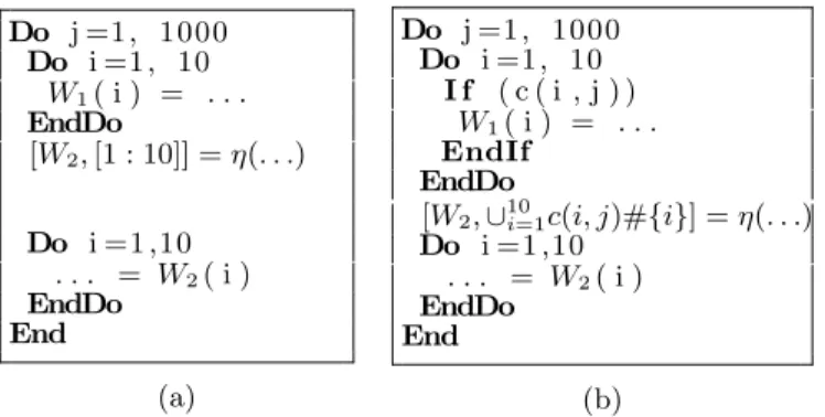
Privatization is a crucial transformation which removes memory related dependences (anti-, and output dependences) and thus allows the parallelization of loops (among other op-timizations). This is achieved by allocating private storage for each iteration3 _{instead of reusing it across the iterations} 3_{In practice, private storage is allocated per thread, and not} per iteration.

Do j =1 , 1000 Do i =1 , 10 W1( i ) = . . . EndDo [W2, [1 : 10]] = η(. . .) Do i =1 ,10 . . . = W2( i ) EndDo End (a) Do j =1 , 1000 Do i =1 , 10 I f ( c ( i , j ) ) W1( i ) = . . . EndIf EndDo

[W2, ∪10i=1c(i, j)#{i}] = η(. . .) Do i =1 ,10

. . . = W2( i ) EndDo

End

(b)

Figure 11: Loop parallelization example. Array W must be privatized. Privatization can be proved at compile-time in (a) and only at run-compile-time in (b).

Algorithm I s C o v e r e d Input: [Au, ℜu] , Loop Output: t r u t h v a l u e Call Search(Au, ℜu, LoopBody )

−−> {[A1, ℜ1], . . . , [An, ℜn], [A0, ℜ0]} Return isEmpty(ℜ0)

Figure 12: Algorithm to decide whether a read is cov-ered by a previous write within every iteration of a given loop.

of a loop. To validate such a transformation, the compiler needs to prove that all read references within some iteration are covered by previous write references to the same memory locations and in the same iteration.

In the example in Fig. 11(a), the parallelization of the outer loop requires the privatization of array W. We must prove that all the reads in the second inner loop are covered by the writes in the first inner loop. Using Array SSA, we can solve this problem by invoking algorithm Search(W2, [1 : 10], LoopBody), which returns {[W1, [1 : 10]], [W0, ∅]}. Since the reference set corresponding to W0 (undefined) is empty, we conclude that all uses of W2 are defined within the same iteration (LoopBody). Therefore privatization of W will remove cross iteration dependences.

In general (Fig. 12), given an array A and a loop Loop, we invoke algorithm Search(Au, ℜU se(Au), LoopBody) for each

use of SSA name Auwithin the loop with footprint ℜU se(Au).

From the result, {[A1, ℜ1], [A2, ℜ2], . . . , [An, ℜn], [A0, ℜ0]}, we are only interested in the value of ℜ0, which is the set of reads not covered by writes, or exposed reads. The priva-tization problem can be formulated as there are no exposed reads, or ℜ0= ∅. In the example in Fig. 11(a), this identity could be proved using symbolic static analysis. However, in the example in Fig. 11(b), the definitions in the first inner loop are controlled by an array of predicates. Depending on their values, there may or may not exist exposed reads. In this case a compile time decision cannot be made. [23] shows how to extract efficient run time tests that prove iden-tities such as ℜ0= ∅ at run time. These run-time tests can extract simple conditions based on partial aggregation and invariant hoisting and generally have lower overhead than the element-by-element run time computation of @ arrays proposed by [16].

5.

IMPLEMENTATION AND

EXPERIMENTAL RESULTS

Our goal is not to prove the profitability of constant prop-agation and array privatization, but to show that they can be implemented easily using Region Array SSA. The pur-pose of this section is to show that, in the cases where con-stant propagation and array privatization can improve the performance of an application, the accurate array dataflow information produced by Region Array SSA makes a signif-icant difference.

We have showed how to use the generic Search algorithm to implement both constant propagation and array privati-zation. However, in some cases it is not necessary to per-form a full search. When perper-forming array privatization, we only need to compute ℜ0, which may be much cheaper than computing the whole list of reaching definitions. When propagating constants, it is not necessary to compute the reaching definition sets that cannot originate from a con-stant assignment. Our implementation takes into account these optimizations.

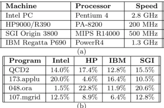
We implemented (1) Region Array SSA construction, (2) the reaching definition algorithm and (3) array constant col-lection in the Polaris research compiler [2], while constant substitution was done by hand because our compiler frame-work lacked some of the necessary infrastructure. We ap-plied constant propagation to four benchmark codes 173.ap-plu, 048.ora, 107.mgrid (from SPEC) and QCD2 (from PER-FECT). The speedups were measured on four different ma-chines (Table 1). The codes were compiled using native compilers at O3 optimization level (O4 on the Regatta). 107.mgrid and QCD2 were compiled with O2 on SGI be-cause the codes compiled with O3 did not validate).

In subroutine OBSERV in QCD2, which takes around 22% execution time, the whole array epsilo is initialized with 0 and then six of its elements are reassigned with 1 and -1. The array is used in loop nest OBSERV do2, where much of the loop body is executed only when epsilo takes value 1 or -1. Moreover, the values of epsilo are used in the inner-most loop body for real computation. From the value set, we discover that the use is all defined with constant 0, 1 and -1. We manually unrolled the loop OBSERV do2, sub-stituted the array elements with their corresponding values, eliminated If branches and dead assignments and succeeded in removing more than 30% of the floating-point multiplica-tions. Additionally, array ptr is used in loops HIT do1 and HIT do2 after it is initialized with constants in a DATA statement. In subroutine SYSLOP, called from within these two loops, the iteration count of a While loop is determined by the values in ptr. After propagation, we can fully unroll the loop and eliminate several If branches.

In 173.applu, a portion of arrays a, b, c, d is assigned with constant 0.0 in loop JACLD do1 and JACU do1. These arrays are only used in BLTS do1 and BUTS do1 (Fig. 10), which account for 40% of the execution time. We find that the uses in BLTS do1 and BUTS do1 are defined as constant 0.0 in JACLD do1 and JACU do1. Loops BLTS do1111 to BLTS do1114 and BUTS do1111 to BUTS do1114 are un-rolled. After unrolling and substitution, 35% of the multi-plications are eliminated.

Machine Processor Speed Intel PC Pentium 4 2.8 GHz HP9000/R390 PA-8200 200 MHz SGI Origin 3800 MIPS R14000 500 MHz IBM Regatta P690 PowerR4 1.3 GHz

(a)

Program Intel HP IBM SGI QCD2 14.0% 17.4% 12.8% 15.5% 173.applu 20.0% 4.6% 16.4% 10.5% 048.ora 1.5% 22.8% 11.9% 20.6% 107.mgrid 12.5% 8.9% 6.4% 12.8%

(b)

Table 1: Constant propagation results. (a) Experimen-tal setup and (b) Speedup.

Program Coverage 1 proc 2 procs 4 procs

S D

ADM 46% 44% -3.5% 78% 216% BDNA 32% 0% -11.9% 71% 225% DYFESM 0% 9% -4.5% 75% 177% MDG 4% 91% -2.0% 91% 263%

Table 2: Array privatization results. Speedup after au-tomatic parallelization on 1, 2 and 4 processors on an SGI Altix machine. The coverage column shows the per-centage of the execution time that could be parallelized only after array privatization. S = at compile time using static analysis, D = at run time using dynamic analysis.

some of its elements are reassigned with constants -2 and -4 before being used in subroutine ABC, which takes 95% of the execution time. The subroutine body is a While loop. The iteration count of the While loop is determined by i1 (there are premature exits). Array a1 is used in ABC after a portion of it is assigned with floating-point constant values. After array constant propagation, the While loop is unrolled and many If branches are eliminated.

107.mgrid was used as a motivating example by previ-ous papers on array constant propagation [30, 24]. Array elements A(1) and C(3) are assigned with constant 0.0 at the beginning of the program. They are used in subroutines RESID and PSINV, which account for 80% of the execution time. After constant propagation, the uses of A(1) and C(3) in multiplications are eliminated.

Table 2 shows the impact of array privatization on the automatic parallelization of major loops in all the applica-tions. In ADM, DYFESM and MDG the privatization prob-lems could be solved only at run time. However, the cost of the run time tests was greatly reduced through partial aggregation of USRs, which led to significant speedups on 2 and 4 processors. The slowdowns on 1 processor are due to the overhead of parallelization and that of run time tests.

6.

RELATED WORK

Array Data Flow. There has been extensive research on array dataflow, most of it based on reference set sum-maries: regular sections (rows, columns or points) [4] linear constraint sets [26, 12, 11, 3, 28, 18, 21, 17, 22, 15, 14, 9, 19, 7, 30, 23], and triplet based [13]. Most of these approaches

approximate nonlinear references with linear ones [17, 9]. Nonlinear references are handled as uninterpreted func-tion symbols in [22], using symbolic aggregafunc-tion operators in [23] and based on nonlinear recurrence analysis in [14]. [8] presents a generic way to find approximative solutions to dataflow problems involving unknowns such as the iter-ation count of a while statement, but limited to intrapro-cedural contexts. Conditionals are handled only by some approaches (most relevant are [28, 17, 13, 19, 23]). Extrac-tion of run-time tests for dynamic optimizaExtrac-tion based on data flow analysis is presented in [19, 23].

Array SSA and its use in constant propagation and parallelization. In the Array SSA form introduced by [16, 24], each array assignment is associated a reference descriptor that stores, for each array element, the iteration in which the reaching definition was executed. Since an array definition may not kill all its old values, a merge func-tion φ is inserted after each array definifunc-tion to distinguish between newly defined and old values. This Array SSA form extends data flow analysis to array element level and treats each array element as a scalar. However, their representa-tion lacks an aggregated descriptor for memory locarepresenta-tion sets. This makes it in generally impossible to to do array data flow analysis when arrays are defined and used collectively in loops. Constant propagation based on this Array SSA can only propagate constants from array definitions to uses when their subscripts are all constant. [7, 6] independently introduced Array SSA forms for explicitly parallel programs. Their focus is on concurrent execution semantics, e.g. they introduce π gates to account for the out-of-order execution of parallel sections in the same parallel block. Although [6] mentions the benefits of using reference aggregation they do not implement it.

Array constant propagation can be done without using Ar-ray SSA [30, 25]. However, we believe that our ArAr-ray SSA form makes it easier to formulate and solve data flow prob-lems in a uniform way.

Table 3 presents a comparison of some of the most relevant related work to Region Array SSA. The table shows that RA SSA is the only representation of data flow that is ex-plicit (uses SSA numbering), is aggregated, and can be com-puted efficiently at both compile-time and run-time even in the presence of nonlinear memory reference patterns. The precision of RA SSA is not as good as that of the other two SSA representations because we lack iteration vector information. However, iteration vectors would become very complex in interprocedural contexts (they must include call stack information), whereas USRs represent arbitrarily large interprocedural program contexts in a scalable way.

7.

CONCLUSIONS AND FUTURE WORK

We introduced a region based Array SSA providing accu-rate, interprocedural, control-sensitive use-def information at array region level. Furthermore, when the data flow prob-lems cannot be completely solved statically we can continue the process dynamically with minimal overhead. We used RA SSA to write a compact Reaching Definitions algorithm that breaks up an array use region into subregions corre-sponding to the actual definitions that reach it. The imple-mentation of array constant propagation and array privati-zation shows that our representation is powerful and easy to use.

RA SSA Array SSA [24] Dist. Array SSA [6] Fuzzy Dataflow [8] Predicated Dataflow [19]

SSA Form Yes Yes Yes No No

Aggregated Yes No No Yes Yes

Static/Dynamic CT/RT CT/RT CT/RT CT CT/RT

Interprocedural Yes No No No Yes

Accuracy Statement Operation Operation x Thread Operation Statement

CT Nonlinear Yes No No Yes No

RT Nonlinear Yes Yes Yes No No

Table 3: Related work on array dataflow and array SSA. CT/RT Nonlinear = able to solve problems involving nonlinear reference patterns at compile time / run time.

8.

REFERENCES

[1] R. A. Ballance, A. B. Maccabe, and K. J. Ottenstein. The Program Dependence Web: A representation supporting control-, data-, and demand-driven interpretation of imperative languages. In ACM PLDI, White Plains, NY, 1990.

[2] W. Blume, et. al. Advanced Program Restructuring for High-Performance Computers with Polaris. IEEE Computer, 29(12):78–82, December 1996.

[3] M. Burke. An interval-based approach to exhaustive and incremental interprocedural data-flow analysis. ACM TOPLAS., 12(3):341–395, 1990.

[4] D. Callahan and K. Kennedy. Analysis of

interprocedural side effects in a parallel programming environment. In Supercomputing: 1st Int. Conf., LNCS 297, pp. 138–171, Athens, Greece, 1987. [5] L. Carter, B. Simon, B. Calder, L. Carter, and

J. Ferrante. Predicated static single assignment. In IEEE PACT ’99, pp. 245, Washington, DC, 1999. [6] D. R. Chakrabarti and P. Banerjee. Static single

assignment form for message-passing programs. Int. J. of Parallel Programming, 29(2):139–184, 2001. [7] J.-F. Collard. Array SSA for explicitly parallel

programs. In Euro-Par, 1999.

[8] J.-F. Collard, D. Barthou, and P. Feautrier. Fuzzy array dataflow analysis. In PPOPP ’95, pp. 92–101, New York, NY, USA, 1995. ACM Press.

[9] B. Creusillet and F. Irigoin. Exact vs. approximate array region analyses. In LCPC, LNCS 1239, pp. 86–100, San Jose, CA, 1996.

[10] R. Cytron, et al An efficient method of computing static single assignment form. In 16th ACM POPL, pp. 25–35, Austin, TX., Jan. 1989.

[11] P. Feautrier. Dataflow analysis of array and scalar references. Int. J. of Parallel Programming, 20(1):23–54, 1991.

[12] T. Gross and P. Steenkiste. Structured dataflow analysis for arrays and its use in an optimizing compilers. Software: Practice & Experience, 20(2):133–155, 1990.

[13] J. Gu, Z. Li, and G. Lee. Symbolic array dataflow analysis for array privatization and program parallelization. In Supercomputing ’95, pp. 47. ACM Press, 1995.

[14] M. R. Haghighat and C. D. Polychronopoulos. Symbolic analysis for parallelizing compilers. ACM TOPLAS, 18(4):477–518, 1996.

[15] M. H. Hall, S. P. Amarasinghe, B. R. Murphy, S.-W.

Liao, and M. S. Lam. Detecting coarse-grain parallelism using an interprocedural parallelizing compiler. In Supercomputing ’95, pp. 49, 1995. [16] K. Knobe and V. Sarkar. Array SSA form and its use

in parallelization. In ACM POPL, pp. 107–120, 1998. [17] V. Maslov. Lazy array data-flow dependence analysis. In ACM POPL, pp. 311–325, Portland, OR, Jan. 1994. [18] D. E. Maydan, S. P. Amarasinghe, and M. S. Lam.

Array data-flow analysis and its use in array privatization. In ACM POPL, pp. 2–15, Charleston, SC, Jan. 1993.

[19] S. Moon, M. W. Hall, and B. R. Murphy. Predicated array data-flow analysis for run-time parallelization. ACM ICS, pp. 204–211, Melbourne, Australia, 1988. [20] Y. Paek, J. Hoeflinger, and D. Padua. Efficient and

precise array access analysis. ACM TOPLAS, 24(1):65–109, 2002.

[21] W. Pugh and D. Wonnacott. An exact method for analysis of value-based array data dependences. In LCPC 1993, LNCS 768, pp. 546–566, Portland, OR. [22] W. Pugh and D. Wonnacott. Nonlinear array

dependence analysis. UMIACS-TR-94-123, Univ. of Maryland, College Park, MD, USA, 1994.

[23] S. Rus, J. Hoeflinger, and L. Rauchwerger. Hybrid analysis: static & dynamic memory reference analysis. Int. J. of Parallel Programming, 31(3):251–283, 2003. [24] V. Sarkar and K. Knobe. Enabling sparse constant

propagation of array elements via array ssa form. In SAS, pp. 33–56, 1998.

[25] N. Schwartz. Sparse constant propagation via memory classification analysis. TR1999-782, Dept. of Compute Science, Courant Institute, NYU, March, 1999. [26] R. Triolet, F. Irigoin, and P. Feautrier. Direct

parallelization of Call statements. In ACM Symp. on Comp. Constr., pp. 175–185, Palo Alto, CA, June 1986.

[27] P. Tu and D. Padua. Gated SSA–based demand-driven symbolic analysis for parallelizing compilers. In 9th ACM ICS, Barcelona, Spain, pp. 414–423, July 1995. [28] P. Tu and D. A. Padua. Automatic array privatization.

In LCPC, LNCS 768 Portland, OR, 1993. [29] P. Vanbroekhoven, G. Janssens, M. Bruynooghe,

H. Corporaal, and F. Catthoor. Advanced copy propagation for arrays. In LCTES ’03, pp. 24–33, New York, 2003.

[30] D. Wonnacott. Extending scalar optimizations for arrays. In LCPC ’00, LNCS 2017, pp. 97–111.