Proton Exchange Membrane Fuel Cells Prognostic Strategy Based on Navigation Sequence Driven Long Short-term Memory Networks

HAL Id: hal-03150117

https://hal.archives-ouvertes.fr/hal-03150117

Submitted on 23 Feb 2021

HAL is a multi-disciplinary open access

archive for the deposit and dissemination of

sci-entific research documents, whether they are

pub-lished or not. The documents may come from

teaching and research institutions in France or

abroad, or from public or private research centers.

L’archive ouverte pluridisciplinaire HAL, est

destinée au dépôt et à la diffusion de documents

scientifiques de niveau recherche, publiés ou non,

émanant des établissements d’enseignement et de

recherche français ou étrangers, des laboratoires

publics ou privés.

Proton Exchange Membrane Fuel Cells Prognostic

Strategy Based on Navigation Sequence Driven Long

Short-term Memory Networks

Chu Wang, Zhongliang Li, Rachid Outbib, Dongdong Zhao, Douman Feng

To cite this version:

Chu Wang, Zhongliang Li, Rachid Outbib, Dongdong Zhao, Douman Feng. Proton Exchange

Mem-brane Fuel Cells Prognostic Strategy Based on Navigation Sequence Driven Long Short-term Memory

Networks. 46th Annual Conference of the IEEE Industrial Electronics Society (IECON 2020), Oct

2020, Singapour, Singapore. pp.3969-3974, �10.1109/IECON43393.2020.9255373�. �hal-03150117�

XXX-X-XXXX-XXXX-X/XX/$XX.00 ©20XX IEEE

Proton Exchange Membrane Fuel Cells Prognostic

Strategy Based on Navigation Sequence Driven

Long Short-term Memory Networks

Chu Wang1,2, Zhongliang Li1, Rachid Outbib1, Dongdong Zhao2, Douman Feng2

1

LIS Lab (UMR CNRS 7020), Aix-Marseille Université, 13397 Marseille, France

2

School of Automation, Northwestern Polytechnical University, 710072 Xi’an, China [email protected]

Abstract—The prognostic of proton exchange membrane

fuel cells (PEMFCs) degradation and the estimation of its remaining useful life (RUL) are effective ways to improve the reliability of the target system and reduce maintenance costs, which is of great significance for the wide commercialization of PEMFCs. Many factors cause the degradation of PEMFCs, and these factors are often difficult to measure accurately. The prognostic method based on long short-term memory networks (LSTMs) has better memory ability for time series and has been demonstrated able to describe the degradation trend of PEMFCs. However, the traditional LSTM prediction algorithm seems to easily fall into the local optimal solution in long-term prediction cases. Overfitting like errors may result in an imprecise or even unstable prognostic. This paper proposes a novel method, named navigation sequence driven LSTMs (NSD-LSTMs), to enhance the accuracy of PEMFCs degradation trend prediction. Two types of PEMFCs aging test data under different load conditions were used to verify the performance of NSD-LSTMs. Experimental results show that, compared with traditional LSTMs, NSD-LSTMs can improve the accuracy of trend prediction. Accurate degradation prognostic can be used to predict RUL and provide guidance for the commercial application of PEMFCs.

Keywords—PEMFCs, Prognostic, NSD-LSTMs, Degradation trend

I. INTRODUCTION

Fuel cells (FCs) are considered to be an energy conversion system that has received widespread attention. Compared with traditional fossil fuels, FCs can greatly reduce environmental pollution. At present, among different types, proton exchange membrane fuel cells (PEMFCs) are one of the most widely used ones [1]. In particular, PEMFCs can convert chemical energy into electrical energy without generating greenhouse gases during their work. This makes PEMFCs suitable for use in transportation represented by electric vehicles [2]. However, for PEMFCs used in electric vehicles, many factors affect degradation in the process of energy conversion. At the same time, electric vehicles often have to face different operating conditions and loads, which results in the remaining useful life (RUL) of PEMFCs often failing to meet the demand [3, 4]. In order to better understand the degradation trend of PEMFCs and facilitate condition-based maintenance and/or control for PEMFCs health management, it is essential to estimate the remaining life of PEMFCs as accurately as possible.

The degradation prediction methods for PEMFCs are mainly categorized as model-driven and data-driven ones. Model-based methods describe the degradation of FCs by building analytical degradation models. The authors in [5],

proposed a multi-agent prediction method based on particle filter (PF) for three parallel PEMFCs. However, only a physical model PF method was considered in this work. In [6], the authors proposed a reconstructed RUL prediction model of FCs, which is used to estimate the RUL of city bus FCs. In this work, the FCs voltage deviation model was built by analyzing different operating conditions of the FCs bus. The authors of [7] proposed a prognostic model based on adaptve unscented Kalman filter (AUKF) for PEMFCs. This model estimated the health state and the RUL by improving the initial parameters setting of conventional UKF.

In practice, model-driven prediction methods are difficult to implement since an analytical degradation model with sufficient fidelity is often hard to build. Data-driven methods have been attracting wider attention compared with model-driven ones, thanks to their light physical model dependency. Especially, inspired by the recent remarkable advances in deep neural networks (NNs), special attention has been put on the development of data-driven prognostic tools by configuring and training different NNs structures. Li et al. [8] used a low-power PEMFCs to conduct long-term experiments in different operating modes, and extracted health indicators (HI) using a sliding adaptive data prediction strategy. The echo state network (ESN) is used to predict the degradation trend and estimate the RUL. Hua et al. proposed a multi-input multi-output echo state network (MIMO-ESN) structure to consider the effects of operating parameters in RUL prediction [9]. In [10], Ma et al. Proposed a recurrent neural network (RNN) structure based on grid long-term short-term memory (G-LSTM) for FC prognostics. The degradation trend of FCs is predicted through short-term and long-term degradation data sets. In the LSTM framework, Liu et al. proposed the use of equal interval sampling and local weighted regression dispersion smoothing method to reconstruct and smooth the data [11].

Among different NNs structures, LSTM has been considered as an effective tool to handle time series prediction problems. For FC prognostics, thanks to the special "gate" structure, well-tuned LSTMs should have the potential to "forget" the abnormal disturbances during stack degradation and "remember" the long-term downward trend of FC performance. However, LSTMs using traditional training protocols are prone to local overfitting, which may lead to significant accumulated errors in multi-step predictions. This work is dedicated to solving the overfitting-like problem of LSTMs and make LSTMs more suitable for long-term prognostic use. Specifically, in this work, an autoregressive integrated moving average model with exogenous variables (ARIMAX) is proposed to generate a navigation sequence (NS) to guide LSTMs for multi-step

prediction. As a consequence, a novel navigation sequence driven LSTMs (NSD-LSTM) prognostic strategy design is proposed. The strategy is then tested using static and dynamic data sets. The results show that the NSD-LSTM based prognostic model has outperformed the classical LSTM methods. The novel training protocol can significantly improve the robustness of LSTM in long-term prediction.

The organization of the paper is as follows. In Section II, the principles of LSTMs and ARIMAX are briefly introduced. The prognostic strategy of NSD-LSTMs is also presented in the same section. In Section III, FCs aging experiments and data set preprocessing are introduced. Then, the proposed prognostic strategy is tested and compared with classical methods. Finally, the work is concluded in Section IV.

II. PROGNOSTIC STRATEGY BASED ON NSD-LSTMS. A. LSTMs Structure

The degradation process of FCs often lasts more than 2,000 hours. Even in some application scenarios, FCs will undergo more than 6,000 hours of degradation process. However, during this longer degradation cycle, the FCs stack output voltage tends to decline very slowly. LSTMs can selectively store long-term data and capture the correlation between time series data. This is also the reason why LSTMs are used to predict the degradation of FCs. In this work, the measured output voltage of FCs is used as the input time series of LSTMs.

Unlike the feedforward neural network, the output of the hidden layer unit in the recurrent neural network (RNN) enters its upper layer network as an input, and also serves as the input of the hidden layer in the next time step. Therefore, the information in the time series data can be continuously retained. RNN has made breakthroughs in many natural language processing projects. Traditional RNN mostly uses backpropagation through time (BPTT) algorithm. The disadvantage of this algorithm is that the increase in the number of network layers will cause problems such as gradient disappearance or gradient explosion with time. LSTMs are an important improved model developed on the basis of RNN. The core essence of LSTMs is that through the introduction of ingenious and controllable self-circulation, a path is created that allows the gradient to flow continuously for a long time. This makes it possible to track information over a longer period, and has become a deep learning model particularly suitable for processing time-series related tasks.

× σ tanh xt-1 ht-1 ct-1 σ × + × tanh σ × σ tanh xt ht ct σ × + × tanh σ × σ tanh xt+1 ht+1 ct+1 σ × + × tanh σ

t-1

t+1

Fig. 1. The repeating units in LSTMs.

As shown in Fig. 1, the key to LSTMs is the cell state (ct).

The horizontal line at the top reflects the operation of ct. This

process can be likened to a conveyor belt, through some smaller linear interactions to achieve chain-like information transfer. LSTMs have a special gate structure that can carefully adjust the information that needs to be deleted and added in the unit. The gate is composed of sigmoid function

(σ), hyperbolic tangent function (tanh) and dot product operation. An LSTM unit contains three such gate structures, called forget gate (ft), input gate (it) and output gate (ot), to

complete the maintenance and control of ct.

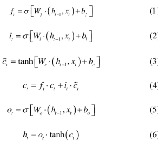
Equations (1) to (6) show the functional equations of LSTMs.  f_t _W_f

















 

where, Wf, Wi, Wc and Wo are weight matrix, bf, bi, bc and bo

are offset terms, ht and xt are the output vector and input

vector of the current unit, (ht-1, xt) indicates that the output

vector (ht-1) of the previous unit is connected to xt to form a

longer vector, c_t is the state of the input unit generated according to xt.

B. ARIMAX Mathematical Model

For a complex system like FCs, the use of a multivariate time series analysis model when constructing its prognostic strategy can potentially enhance the prognostic performance. The ARIMAX model is one of the most commonly used multivariate time series analysis models, which can be used to explain the relationship between system variables. In the long-term prediction, compared with the multilayer perceptron artificial neural network (MLP ANN), adaptive neuro-fuzzy inference systems (ANFIS) and support vector machine (SVM), thanks to the addition of exogenous sequences, the ARIMAX model shows better prediction accuracy [12]. The following is a simplified ARIMAX mathematical model:          1 it k li i i i t t t t B B B B B x y a                    

where yt, xit and



variable sequence and random error sequence, respectively.

 

i B

 denotes the auto-regression coefficients' multinomial of the i-th input time series, i B denotes the average coefficients' multinomial of the i-th input time series, li represents the lag degree of the i-th independent variables,

 B

 denotes residual series' moving average coefficients' multinomial,  B denotes residual series' auto-regression

coefficients' multinomial, and {at} is white noise time series

with zero average.

The prediction process of ARIMAX model is shown in Fig. 2. The training set and the exogenous sequence should be standardized before fitting the ARIMAX model, so that

the data can be more easily predicted. Then, the data is input to the ARIMAX model as training data. The trained ARIMAX model is used to predict the next m hours of data. Finally, the actual prediction data is obtained through inverse standardization [13].

Training set Standardized data Fit ARIMAX model Predict the next m hours Inverse standardized of predicted data Actual prediction sequence Exogenous sequence

Fig. 2. The prediction process of ARIMAX model.

C. The Prognostic Strategies of NSD-LSTMs

When FCs are used in dynamic load scenarios such as electric vehicles, the start-stop process of FCs will cause their stack voltage degradation trend to show large fluctuations in a short period of time [8]. Although LSTMs can selectively forget the unnecessary voltage fluctuations in the long-term change trend of FCs stack voltage during time series processing, the large-scale fluctuations of the short-term voltage mentioned above are still easy to cause LSTMs to fall into the error of local overfitting. Therefore, this paper proposes a novel prognostic strategy that takes into account the characteristics of LSTMs and ARIMAX.

The Prognostic Strategies of NSD-LSTMs

Offline phase Online phase Stack voltage dataset Dataset preprocessing

Training set Test set Predicted voltage degradation trends Predicted RUL Actual RUL ARIMAX model Exogenous sequence Navigation Sequence Train LSTMs by different initial values LSTMs 1 LSTMs 2 LSTMs n •• • NSD-LSTMs Multi-step prediction NSD-LSTMs 1 NSD-LSTMs 2 NSD-LSTMs n •• •

Fig. 3. The prognosis strategy based on NSD-LSTMs.

The prognostic strategy based on NSD-LSTMs is shown in Fig. 3. In this work, the NSD-LSTMs prognostic strategy is developed to predict FC stack voltage evolution. The datasets used to test the proposed strategy were obtained from FCs aging experiments. Before the implementation of the prognostic strategy, each dataset is divided into training and test sets. The operation process of NSD-LSTMs prognostic strategy is implemented in two phases, i.e. offline and online phases. The test set is considered completely unknown whether in the online phase or offline phase. When verifying the accuracy of the prognostic strategy, the test set is used to generate the actual RUL.

Offline training phase: The offline phase, which is displayed on the left half of the bottom of Fig. 3. This phase contains two parts: generating NS and training LSTMs.  Generating NS

1) Generate exogenous sequences. Specifically, the exogenous sequence is obtained by filtering the training set using locally weighted scatterplot smoothing (LOESS) method [11]. It can be found that in Fig. 4, the exogenous sequence reduces some large voltage fluctuations compared

with the training set, and the exogenous sequence also retains the long-term degradation trend of the stack voltage.

2) As shown in Fig. 4, the NS is generated by simultaneously inputting two time series, the training set and the exogenous sequence, into the ARMIAX model. For a dataset, NS is unique and fixed.

0 2000 4000 6000 8000 10000 480 500 520 540 560 580 600 620 640 660 Stack voltage (mV) Time (h) Training set Test set Exogenous sequence Navigation sequence

Training set Test set

Fig. 4. The stack voltage dataset.

 Training LSTMs

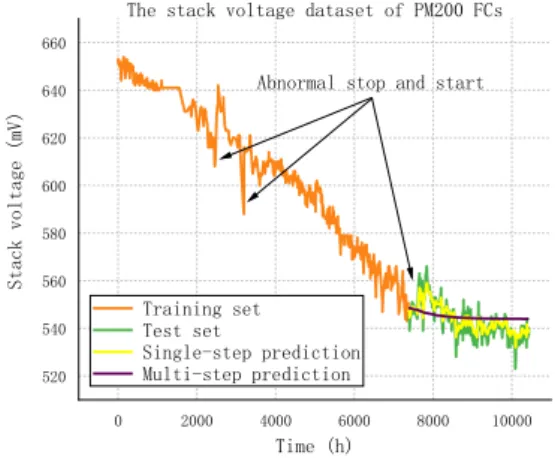
In the proposed prognostic strategy, ADAM is used as an optimizer to train LSTMs [14]. By setting multiple initialization parameters randomly in ADAM, multiple LSTMs can be trained to generate multiple prognostic models, as LSTMs 1, LSTMs 2, ..., LSTMs n shown in Fig. 3. The multiple LSTMs setting benefits to provide diverse prediction results, which will be used further to evaluate prediction uncertainty. 0 2000 4000 6000 8000 10000 520 540 560 580 600 620 640 660 Stack voltage (mV) Time (h) Training set Test set Single-step prediction Multi-step prediction

The stack voltage dataset of PM200 FCs

Abnormal stop and start

Fig. 5. Single-step prediction and multi-step prediction of LSTMs.

Online predicting phase: As shown in the green frame of Fig. 3, the prediction of stack voltage degradation trend and RUL prediction are completed in the online phase. The trained LSTMs model can perform single-step prediction and multi-step prediction, as shown in Fig. 5. In this study, an iterative single-step prediction is deployed to achieve multi-step prediction of FC stack voltage. As in each single-multi-step prediction, the previous predicted value s fed to LSTMs models, the prediction error will be accumulated with the prediction steps. In this study, NS is added to the avalable training data to assist LSTMs in the multi-step prediction

process and limit the accumulated error. In the online phase, multiple multi-step prediction models (NSD-LSTMs 1, NSD-LSTMs 2,..., NSD-LSTMs n) are trained at each prediction instant. These multi-step models will give n different voltage degradation prediction results. Assuming that the predictions of multiple NSD-LSTMs models follow the standard Gaussian distribution, the confidence interval (CI) is configured as 95% probability interval [8], and the average value of the predicted values is regarded as the final predicted voltage degradation trend. The RUL is estimated by comparing the predicted degradation trend with a predetermined failure threshold. At the same time, the CI of RUL is also set to 95%.

III. FCS AGING EXPERIMENT AND EVALUATION OF PROGNOSTIC STRATEGY

A. FCs Aging Experiment

In this paper, through two long-term aging experiments of FCs, the stack voltage degradation trend datasets, which are also used to predict the corresponding RUL, were constructed.

1). Constant load aging experiment

The FCs aging experiment of the constant load is completed on 1kW Proton Motor 200 (PM200) fuel cell. In this experiment, the PM200 FC stack with 96 cells was tested under the operating conditions shown in TABLE I.

TABLE I. CONSTANT LOAD AGING EXPERIMENTS OPERATING

CONDITION

Operating mode Constant load Air supply Air blower & filter Cooling system DI-water/glycol Fuel gas supply 99.99% dry [email protected] bar Number of cells 96

Operating hours 10430 h Stack temp. 58 °C Current density 0.64 A/cm2

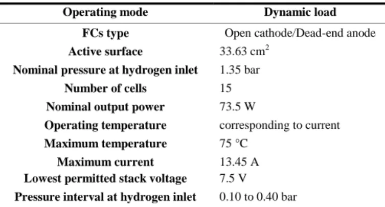
2). Dynamic load aging experiment

TABLE II. DYNAMIC LOAD AGING EXPERIMENTS OPERATING

CONDITION

Operating mode Dynamic load

FCs type Open cathode/Dead-end anode Active surface 33.63 cm2

Nominal pressure at hydrogen inlet 1.35 bar

Number of cells 15

Nominal output power 73.5 W

Operating temperature corresponding to current Maximum temperature 75 °C

Maximum current 13.45 A

Lowest permitted stack voltage 7.5 V Pressure interval at hydrogen inlet 0.10 to 0.40 bar

In the dynamic load aging experiment, the FC stack is designed as an open cathode and a dead-end anode structure. Some operating conditions are shown in TABLE II. A 24V DC fan realizes the functions of air supply and temperature adjustment. The hydrogen pressure as fuel is fixed at about 1.35 bar. In addition, FCs are self-humidifying and a purge lasting for 0.5 seconds is activated every 30 seconds. In order to get closer to the dynamic operating conditions of FCs in

electric vehicle applications, a programmable electronic DC load was used to set the output current in the experiment. B. Dataset Preprocessing

The data set of FCs stack voltage can be found in Fig. 5 and Fig. 6, where the abnormal voltage fluctuation occurs in the marked positions. These abnormalities are caused by the stops and starts of FCs due to peripheral equipment failure or fuel replacement. To test the prognostic performance of the proposed strategy, from 50% to 90% of final time instant, the prediction time points are placed with increment of 1%. That means that prognostic procedure is implemented for 40 times for each dataset. For instance, a prognostic point is set at 70% instant, the part before the point is called the training set, and the part after the point is called the test set.

-200 0 200 400 600 800 1000 1200 1400 1600 8.0 8.5 9.0 9.5 10.0 10.5 Stack voltage (V) Time (h) Stop caused by replacement of hydrogen tank Dynamic load FCs

Fig. 6. Dataset of stack voltage of dynamic load FCs.

C. Evaluation Criteria

It is necessary to formulate evaluation criteria for prognostic strategies, which can accurately and comprehensively evaluate a prediction model. This article sets two evaluation criteria, the root-mean-square error (RMSE) and the relative error (RE), where RMSE evaluates the training effect of the LSTMs model in the offline phase, and RE is used in the online phase to evaluate the accuracy of the RUL given by the prognostic strategy. The mathematical description of RMSE and RE can be found in equations (8)-(9) 







where, yj is the actual stack voltage observation value in the

test set, and yj is the predicted voltage value output by the

trained LSTMs model in the offline phase.

 RE RULRUL RUL100% 

where, RUL is the actual RUL generated by the test set, and

RUL is the RUL predicted by the proposed prognostic strategy.

D. Prognostic Experiment and Discussion

The program code used in the FCs prognostic experiment was developed in Matlab R2019b. The specific operating

environment is as follows. Central Processing Unit (CPU): Intel (R) Core (TM) i5-3230M CPU @ 2.60GHz; memory capacity (type): 8 GBytes (DDR3); operating system: Microsoft Windows 7 (64-bit).

1) Evaluation of LSTMs prediction model

The training hyperparameters of LSTMs are configured similarly to a regular NNs. The ADAM optimizer is selected for training the LSTMs model, and the number of hidden units is set to 200. The mini batch size is specified as 64, and the maximum training epoch is 150. To avoid gradient explosion, the gradient threshold is set to 1. The initial learning rate is specified as 0.001, and after 125 epochs training, the learning rate is reduced by multiplying by a factor of 0.2.

Fig. 7. LSTMs single-step prediction.

Fig. 8. RMSE of prediction result.

By comparing the single-step predicted voltage value with the observed voltage value in the test set and calculating the RMSE, the predicted performance of the trained LSTMs model is evaluated. As shown in Fig. 7 and Fig. 8, the single-step prediction results under constant load operating conditions when the split point between training and test data is selected to be 50%. The prediction results show that the RMSE of the prediction results of the LSTMs model is 0.0079686, which is acceptable for an aging experiment with a total operating time of 14,300 hours. By changing the split point, multiple tests were conducted to verify the accuracy of the LSTMs model prediction. It is worth mentioning that this test can also be modified to set the parameters of LSTMs in the offline phase. The same test was also performed on the dynamic load FCs dataset and presented a consistent conclusion.

2) Evaluation of NSD-LSTMs Prognostic model

Limited by paper length, only results concerning dynamic data are presented and discussed in the sequel. The NSD-LSTMs models were used to perform 20 prognostic experiments at the 57% split point. As shown in Fig. 9, colored lines represent the results of multiple prognostic. The prognostic results can be summarized as the following three points: First, multiple prognostic results show ideal consistency, which shows that the proposed prognostic model can work stably. Second, in the vicinity of the split point, the prognostic results have decreased significantly, this is because NS played a guiding role. At the same time, this also seems to be related to the severe voltage fluctuations before the split point. Third, the prognostic models remember the potential voltage degradation trends in the training set, and filter out useless voltage fluctuation details.

Fig. 9. Multiple prognostic through NSD-LSTMs model.

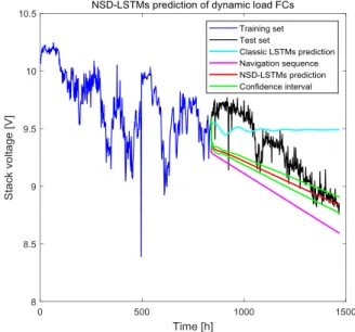
At each time point in the prediction phase, the average and CI of multiple prognostic results are calculated. As shown in Fig. 10, the red line is the average value, which is the final predicted degradation trend, and the green line represents the upper and lower limits of CI. The cyan line is the degradation trend predicted by the classic LSTMs model, and the magenta line is the NS generated by the ARIMAX model. The time required for the predicted degradation trend to reach the threshold is recorded, which is noted as the predicted RUL.

Fig. 10. Prediction of FCs stack voltage degradation trend.

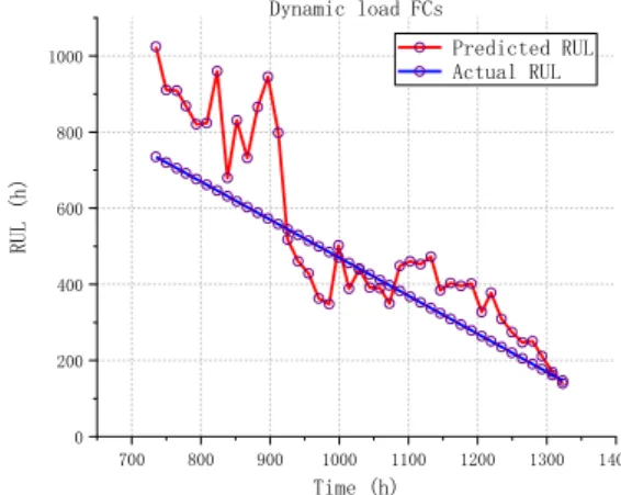
The prediction time slides from 50% to 90% of the whole data time horizon with an increment of 1%. The RUL can be

estimated at each prediction time, as shown in Fig. 11. The RE can be calculated accordingly in combination with the actual RUL, as shown in Fig. 12. The results show that RE shows an related trend of fluctuations. The smallest RE in the test results is 0.34%, which means that the RUL prediction accuracy rate at this time is 99.66%.

700 800 900 1000 1100 1200 1300 1400 0 200 400 600 800 1000 RUL (h) Time (h) Predicted RUL Actual RUL Dynamic load FCs

Fig. 11. RUL prediction at different moments.

50 60 70 80 90 0 10 20 30 40 50 60 70 RE (%) Split point (%) RE

Fig. 12. The RE of the predicted RUL

IV. CONCLUSION

This paper presents an NSD-LSTMs prognostic model. This prognostic strategy can assist in the prediction of stack voltage degradation trends and RUL of FCs in dynamic operating scenarios such as electric vehicles. In order to verify the correctness of the proposed method, the aging experimental data of constant load and dynamic load FCs were used. Under the guidance of NS, the trained LSTMs can obviously better predict the degradation trend of the FCs stack. A series of NSD-LSTMs models generated using different initial values can predict multiple degradation trends and show appropriate consistency. By testing the proposed prognostic models with real experimental data, it

shows that the proposed model can accurately predict the RUL of FCs and provide reliable reference information in different operating conditions.

ACKNOWLEDGMENT

The author Chu Wang acknowledges the financial support from the China Scholarship Council (File No. 201906290107).

REFERENCES

[1] V. Das, S. Padmanaban, K. Venkitusamy, R. Selvamuthukumaran, F. Blaabjerg, and P. Siano, "Recent advances and challenges of fuel cell based power system architectures and control – A review," Renewable and Sustainable Energy Reviews, vol. 73, pp. 10-18, 2017. [2] Z. Hua, Z. Zheng, F. Gao, M. C. Péra, "Challenges of the remaining

useful life prediction for proton exchange membrane fuel cells," in IECON 2019 - 45th Annual Conference of the IEEE Industrial Electronics Society, pp. 6382-6387, 2019.

[3] U. Lucia, "Overview on fuel cells," Renewable and Sustainable Energy Reviews, vol. 30, pp. 164-169, 2014.

[4] O. Z. Sharaf and M. F. Orhan, "An overview of fuel cell technology: Fundamentals and applications," Renewable and Sustainable Energy Reviews, vol. 32, pp. 810-853, 2014.

[5] J. Liu and E. Zio, "Prognostics of a multistack PEMFC system with multiagent modeling," Energy Science & Engineering, vol. 7, no. 1, pp. 76-87, 2019.

[6] Z. Hu, L. Xu, J. Li, M. Ouyang, Z. Song, and H. Huang, "A reconstructed fuel cell life-prediction model for a fuel cell hybrid city bus," Energy Conversion and Management, vol. 156, pp. 723-732, 2018.

[7] H. Liu, J. Chen, C. Y. Zhu, H. Y. Su, and M. Hou, "Prognostics of Proton Exchange Membrane Fuel Cells Using A Model-based Method," Ifac Papersonline, vol. 50, no. 1, pp. 4757-4762, 2017. [8] Z. Li, Z. Zheng, and R. Outbib, "Adaptive Prognostic of Fuel Cells by

Implementing Ensemble Echo State Networks in Time-Varying Model Space," IEEE Transactions on Industrial Electronics, vol. 67, no. 1, pp. 379-389, 2020.

[9] Z. Hua, Z. Zheng, F. Gao, M. C. Péra, "Remaining useful life prediction of PEMFC systems based on the multi-input echo state network," Applied Energy, Mar. 2020, 265: 114791. https://doi.org/10.1016/j.apenergy.2020.114791. In press.

[10] R. Ma, T. Yang, E. Breaz, Z. Li, P. Briois, and F. Gao, "Data-driven proton exchange membrane fuel cell degradation predication through deep learning method," Applied Energy, vol. 231, pp. 102-115, 2018. [11] J. Liu, Q. Li, W. Chen, Y. Yan, Y. Qiu, and T. Cao, "Remaining

useful life prediction of PEMFC based on long short-term memory recurrent neural networks," International Journal of Hydrogen Energy, vol. 44, no. 11, pp. 5470-5480, 2019.

[12] A. Jalalkamali, M. Moradi, and N. Moradi, "Application of several artificial intelligence models and ARIMAX model for forecasting drought using the Standardized Precipitation Index," International Journal of Environmental Science and Technology, vol. 12, no. 4, pp. 1201-1210, 2014.

[13] L.-Y. Chiu, D. J. A. Rustia, C.-Y. Lu, and T.-T. Lin, "Modelling and Forecasting of Greenhouse Whitefly Incidence Using Time-Series and ARIMAX Analysis," Ifac Papersonline, vol. 52, no. 30, pp. 196-201, 2019 2019.

[14] D. P. Kingma and J. Ba, "Adam: A method for stochastic optimization," arXiv preprint arXiv:1412.6980, 2014.