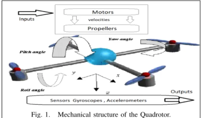
Comparative Study of Control Approaches Designed for a Quadrotor in a Visual Servoing Task without Observers

concepts auxquels recouraient les spécialistes de politique internationale pour analyser celle-ci depuis la fin de la Seconde Guerre mondiale système bipolaire

34 Some ICDAR results of our method: even if the text detection is quite good, p and r statistics are very poor on these images because of ICDAR ground truth.. ICDAR metric Wolf

Then, an adaptive sliding mode controller is synthesized in order to stabilize both bank and pitch angles while tracking heading and altitude trajectories and to compensate

3.2.3 redMaPPer catalogue In the redMaPPer catalogue, we also restrict the sample to those clusters in the 0.1 < z < 0.4 redshift range and with six or more galaxies with

CONCLUSIONS AND FUTURE WORKS This paper presents a vehicle control system for a quadro- tor Micro-UAV based on a combined control strategy in- cluding feedback linearization to

Lorsque le cathéter est laissé en place, dans les recommandations américaines, un traitement antibiotique par voie générale de 10–15 jours associé à un verrou

An approximation of the sign function has been given based on delayed values of the processed variable, which ensures chattering reduction for the sliding mode control and

The challenging problem of active control of separated flows is tackled in the present paper using model-based design principles, and applied to data issued from a