HAL Id: hal-01192732
https://hal.inria.fr/hal-01192732
Submitted on 6 Mar 2018
HAL is a multi-disciplinary open access
archive for the deposit and dissemination of
sci-entific research documents, whether they are
pub-lished or not. The documents may come from
teaching and research institutions in France or
abroad, or from public or private research centers.
L’archive ouverte pluridisciplinaire HAL, est
destinée au dépôt et à la diffusion de documents
scientifiques de niveau recherche, publiés ou non,
émanant des établissements d’enseignement et de
recherche français ou étrangers, des laboratoires
publics ou privés.
Towards Application Variability Handling with
Component Models: 3D-FFT Use Case Study
Vincent Lanore, Christian Pérez, Jérôme Richard
To cite this version:
Vincent Lanore, Christian Pérez, Jérôme Richard. Towards Application Variability Handling with
Component Models: 3D-FFT Use Case Study. UnConventional High Performance Computing 2015,
Jens Breitbart, Technische Universität München, DE; Josef Weidendorfer, Technische Universität
München, DE, Aug 2015, Vienne, Austria. pp.12, �10.1007/978-3-319-27308-2_61�. �hal-01192732�
Towards Application Variability Handling with
Component Models: 3D-FFT Use Case Study
Vincent Lanore?, Christian Perez†, and J´erˆome Richard†
?Ecole Normale Sup´erieure de Lyon,´ †
Inria Avalon Research Team, LIP, Lyon, France
Abstract. To harness the computing power of supercomputers, HPC application algorithms have to be adapted to the underlying hardware. This is a costly and complex process which requires handling many al-gorithm variants. This paper studies the ability of the component model L2C to express and handle the variability of HPC applications. The goal
is to ease application adaptation. Analysis and experiments are done on a 3D-FFT use case. Results show that L2C, and components in general,
offer a generic and simple handling of 3D-FFT variants while obtaining performance close to well-known libraries.
Keywords: Application Adaptation, Component Models, High-Performance Computing
1
Introduction
To harness the computing power of supercomputers, high-performance comput-ing (HPC) applications must have their algorithms adapted to the underlycomput-ing hardware. Adaptation to a new hardware can involve in-depth transformations or even algorithm substitutions because of different scales, features, or communica-tion/computation ratios. Since hardware evolves continuously, new optimizations are regularly devised. As a consequence, application codes must often be tweaked to adapt to new architectures so as to maximize performance; maintainability is rarely taken into account.
Adapting an application code to a specific use has a cost in terms of devel-opment time and requires very good knowledge of both the target platform and the application itself. It might also prove difficult for someone other than the original code developer(s). Moreover, unless automated, adapting the code for a specific run is, in many cases, too costly.
A promising solution to simplify application adaptation is to use component-based software engineering techniques [14]. This approach proposes to build ap-plications by assembling software units with well-defined interfaces; these units are called components. Components are connected to form an assembly. Syn-tax and semantics of interfaces and assemblies are given by a component model. Such an approach enables easy reuse of (potentially third-party) components and simplifies adaptation thanks to assembly modifications. Also, some component models and tools enable automatic assembly generation and/or optimization [5,
8]. Component models bring many software engineering benefits but very few provide enough performance for high-performance scientific applications. Among them is L2C [4], a low-level general purpose high-performance component model
built on top of C++ and MPI.
This paper studies the ability of L2C to handle HPC application variability on a 3-dimensional Fast Fourier Transform (3D-FFT) use case: a challenging numerical operation widely used in several scientific domains to convert signals from a spatial (or time) domain to a frequency domain or the other way round. Our experiments and adaptation analysis show that it is possible to easily spe-cialize 3D-FFT assemblies (hand-written, with high reuse, without delving into low-level code and with as little work as possible) while having performance comparable to that of well-known 3D-FFT libraries.
The paper is structured as follows. Section 2 gives an overview of related work. Then, Section 3 deals with component models and introduces L2C. Section 4
describes the assemblies that we have designed and implemented with L2C for
various flavors of 3D-FFTs. Section 5 compares the 3D-FFT L2C assemblies with
existing FFT libraries both in terms of performance and in terms of reuse/ease of adaptation. Section 6 concludes the paper and gives some perspectives.
2
Related Work
This section briefly discusses related works in HPC application adaptation. For space reasons, only selected relevant publications are presented.
To efficiently run applications on several hardware architectures, it is usually required to have algorithm variants that specifically target each architecture. An efficient variant can then be chosen and executed according to hardware and software characteristics.
Variants and choices can be directly implemented in the application code using conditional compilation or using conditional constructs. But, it leads to a code difficult to maintain and to reuse due to the multiplication of concerns in a same code (e.g., functional and non-functional concerns).
Other approaches rely on compilation techniques to handle variants or choices. Many domain-specific languages (e.g., Spiral [7]) allow the generation of efficient FFT codes but do not allow the application developers to easily handle variants since they are implemented inside compilers or associated frameworks. Some ap-proaches like PetaBricks [1] aim to describe an FFT algorithm in a high-level language and provide multiple implementations for a given piece of function-ality. This enables the expression of algorithms and their variations. However variants can be complex to reuse through multiple applications since it is the responsibility of the developer to support compatibility by providing portable interfaces.
Other approaches such as the FFTW codelet framework [10] and the Open-MPI MCA framework [13] build efficient algorithm implementations by com-posing units such as pieces of code or components for a specific purpose. These approaches solve a problem by decomposing it into smaller problems and use
a set of specialized units to solve each one. These approaches provide some forms of adaptation framework but, to our knowledge, it is not possible to eas-ily integrate new and/or unique optimizations. Also, both these examples are specialized frameworks whose top-level algorithms are difficult to change.
This paper aims to show that components with assembly can be used to adapt HPC applications in a simpler and more generic manner than commonly used approaches.
3
Component Models
3.1 Overview
Component-based software engineering [11] is a programming paradigm that proposes to compose software units called components to form a program. A component model defines components and component composition. A classical definition has been proposed by Clemens Szyperski [14]: A software component is a unit of composition with contractually specified interfaces and explicit context dependencies only. A software component can be deployed independently and is subject to third-party composition. In many component models, interfaces are called ports and have a name. To produce a complete application, components must be instantiated and then assembled together by connecting interfaces. The result of this process is called an assembly. The actual nature of connections is defined by the component model and may vary from one model to another.
Component models help to separate concerns and to increase reuse of third-party software. Separation of concerns is achieved by separating the role of component programming (low-level, implementation details) from component assembly (high-level, application structure). Reuse of third-party components is possible because component interfaces are all that is needed to use a component; it is thus not necessary to be familiar with low-level details of the implementa-tion of a component to use it. Component models also allow different pieces of code to use different implementation of the same service as opposed to libraries. Separation of concerns and reuse would allow to easily mix pieces of codes from different sources to make specialized assemblies. Thus, adaptation would no longer require in-depth understanding of existing implementations (separation of concerns) or re-development of existing optimizations (reuse).
Many component models have been proposed. The CORBA Component Model [6] (CCM) and the Grid Component Model (GCM) [2] are notable ex-amples of distributed models. However, they generate runtime overheads [15] that are acceptable for distributed application but not for HPC. The Common Component Architecture [3] (CCA) is the result of an US DoE effort to enhance composability in HPC. However, CCA is mainly a process-local standard that relies on external models such as MPI for inter-process communication. As a consequence, such interactions do not appear in component interfaces. The Low Level Components [4] (L2C) is a minimalist HPC component model built on top
primitive components, local connections (process local uses/provides ports), MPI connections (MPI communicator sharing), and optionnally remote con-nections (CORBA based uses/provides ports).
As this paper studies the use of L2C to ease HPC applications, the next
section presents L2C in more detail.
3.2 L2C Model
The L2C model is a low level component model that does not hide system is-sues. Indeed, each component is compiled as a dynamic shared object file. At launch time, components are instantiated and connected together according to an assembly description file or to an API.
L2C supports features like C++ method invocation, message passing with
MPI, and remote method invocation with CORBA. L2C components can provide
services thanks to provides ports and use services with uses ports. Component dependencies are inferred from connections between interfaces. Multiple uses ports can be connected to a unique provides port. A port is associated with an object interface and a name. Communication between component instances is done by member function invocations on ports. L2C also provides MPI ports as a
way to share MPI communicators between components. Components can expose attributes used to configure component instances. The C++ mapping defines components as plain C++ classes with a few annotations (to declare ports and attributes). Thus library codes can easily be wrapped into components.
A L2C assembly can be described using a L2C assembly descriptor file (LAD). This file contains a description of all component instances, their attributes values, and the connections between instances. Each component is part of a process and each process has an entry point (an interface called when the application starts). It also contains the configuration of MPI ports.
As described in [4], L2C has been successfully used to describe a stencil-like
application with performance similar to native implementations.
4
Designing 3D-FFT Algorithms with L
2C
This section analyses how L2C, as an example of a HPC component model, can
be used to implement distributed 3D-FFT assemblies. To that end, we have first designed a basic 3D-FFT assembly. Then, we have modified it to incorporate several optimizations. All the assemblies presented here have been implemented in C++/L2C, and relevant assemblies are evaluated in Section 5. Let us first
focus on the methods used to compute a 3D-FFT. 4.1 3D-FFT Parallel Computation Methods
3D-FFT parallel computation can be done using 1D or 2D domain decomposi-tion [12]. The whole computadecomposi-tion can be achieved by interleaving data compu-tation steps and data transposition steps. Compucompu-tation steps involve applying
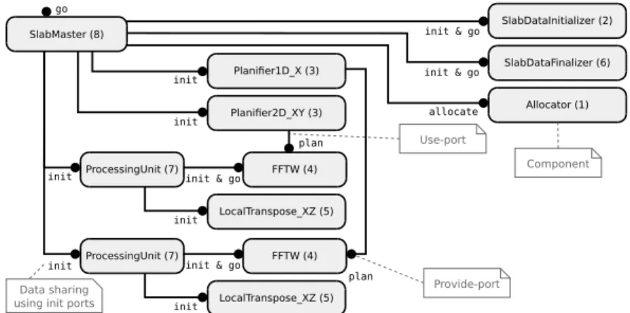
go SlabMaster (8) SlabDataInitializer (2) SlabDataFinalizer (6) ProcessingUnit (7) FFTW (4) Allocator (1) LocalTranspose_XZ (5) init & go init & go allocate init & go Planifier1D_X (3) init plan plan Planifier2D_XY (3) init init init ProcessingUnit (7) FFTW (4) LocalTranspose_XZ (5) init & go init init Component Use-port Provide-port Data sharing
using init ports
Fig. 1: Local (one process) basic 3D-FFT assembly using 1D decomposition.
multiple sequential 1D/2D FFTs. Data transposition can be achieved by using all-to-all global exchanges. Transposition performance is the major bottleneck.
1D decomposition involves 2 local computation steps, and 1 or 2 transpo-sitions depending on the final data layout. For a given cube of data of size N × N × N , this approach is scalable up to N processing elements (PEs) at which point each PE has a slab of height 1.
2D decomposition involves 3 local computation steps, and between 2 and 4 transpositions depending on the final data layout. It scales up to N × N PEs.
To increase 3D-FFT computation performance and to enable a better adap-tation to hardware, a sequential 3D-FFT algorithm variant can be selected at initialization using a planning step. Information about the algorithm selection is stored in a plan that is then executed at runtime.
4.2 Basic Sequential Assembly
Figure 1 displays a single node sequential assembly that implements the 1D-decomposition algorithm presented above. It will be the base for parallel as-semblies. It is based on the identification of 8 tasks that are then mapped to components: 6 for the actual computation, and 2 for the control of the compu-tation. The computation-oriented components implement the following tasks:
1. Allocator: allocate 3D memory buffers. 2. SlabDataInitializer: initialize input data.
3. Planifier1D X and Planifier2D XY: plan fast sequential FFTs.
4. FFTW: compute FFTs (wrapping of FFTW library, with SIMD vectorization). 5. LocalTranspose XZ: locally transpose data.
6. SlabDataFinalizer: finalize output data by storing or reusing it. The two control components implement the following tasks:
8. SlabMaster: drive the application (e.g., initialize/run FFT computations). Task 2 (SlabDataInitializer), 6 (SlabDataFinalizer) and 8 (SlabMaster) are specific to the 1D decomposition. These tasks and Task 5 (LocalTranspose
XZ) are specific to a given parallelization strategy, here sequential. Task 3 (Planifier1D X and Planifier2D XY) and Task 4 (FFTW) are specific to a chosen sequential FFT library (to compute 1D/2D FFT).
All computation-oriented components except Allocator rely on memory buffers. They can use two buffers (i.e., an input buffer and an output buffer) or just one for in-place computation. These buffers are initialized by passing memory pointers during the application startup. For this purpose, these compo-nents provide an init port to set input and output memory pointers, but also to initialize or release memory resources. All computation-oriented components except Allocator provide a go port which is used to start their computation.
As FFT plans depend on the chosen sequential FFT library, Component FFTW (Task 4) exposes a specific Plan interface that is used by Planifier1D X and Planifier2D XY (Task 3). This connection is used to configure the FFT components after the planning phase.
The application works in three stages. The first stage consists in initializing the whole application by allocating buffers, planning FFTs and broadcasting pointers and plans to component instances. In the second stage, the actual com-putation happens, driven by calls on the go ports of component instances in such a manner as to interleave computations and communications. The last stage con-sists in releasing resources such as memory buffers. The whole process is started using the go port of the SlabMaster component.
The assembly has been designed to be configured for a specific computation of a 3D-FFT. Buffer sizes and offsets are described as components attributes; they are not computed at runtime.
4.3 Parallel Assembly for Distributed Architectures
The distributed version of the assembly is obtained by deriving an MPI version of SlabDataInitializer (Task 2), SlabDataFinalizer (Task 6), SlabMaster (Task 8). Basically, it consists in adding a MPI port to them. LocalTranspose XZ components are replaced by MpiTransposeSync XZ which also exhibit MPI ports used for distributed matrix transpositions. Furthermore, this assembly is dupli-cated on each MPI process (with different attributes). MpiTransposeSync XZ in-stances of a same computation phase are interconnected through their MPI ports, so that they share an MPI communicator. It is also the case for SlabMaster, SlabInitializer, and SlabFinalizer instances. Data distribution depends on the chosen decomposition (1D or 2D).
4.4 Assembly Adaptation
This section presents three possible adaptations of the parallel assembly pre-sented above: load balancing for an heterogeneous distributed system, adjust-ments of the number of transpositions, and use of a 2D decomposition.
Heterogeneous Assembly A first example of adaptation is taking into ac-count heterogeneous hardware architectures, such as for example the thin and large nodes of the Curie supercomputer. When all nodes do not compute at the same speed and data is evenly distributed between nodes, the slower nodes limit the whole computation speed due to load imbalance. To deal with this problem, load balancing is needed and thus data must be unevenly distributed between nodes. Since load balancing of 3D-FFTs depends on data distribution, a solution is to control data distribution through component attributes. A new transposi-tion component must be implemented to handle uneven data distributransposi-tion. Thus, handling heterogeneous systems can be easily done by reusing components from the previous section with small modifications.
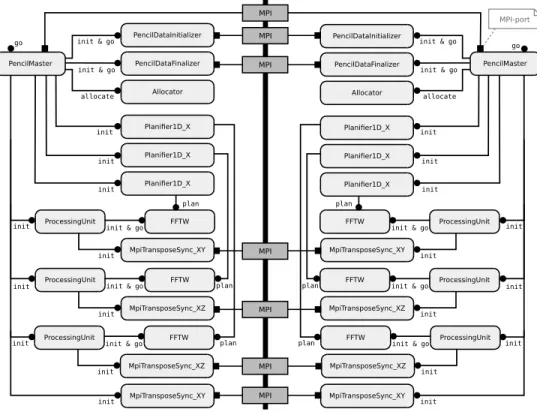
Reducing the Number of Transpositions Optimizing the transposition phase is important as it is often the main bottleneck. As explained in Section 4.1, the final transposition can possibly be removed with 1D decomposition (and up to two transpositions using a 2D decomposition) depending on the desired ori-entation of the output matrix. This can be done by adding an attribute to the Mastercomponent: in each process, the second ProcessingUnit component in-stance connected to the SlabMaster via init and go ports is removed, and the transposition component is connected to it via the same port type; the go and init uses ports of the SlabMaster component are directly connected to the associated provides ports of components implementing the Task 4 of the last phase. As the SlabMaster behavior during the initialization depends on whether a final transposition is used or not (the final buffer differs), a boolean attribute is added to the SlabMaster to configure it. So, the number of transpositions can be easily adjusted using assembly adaptation and component replacement. 2D Decomposition Assembly 2D decomposition assemblies are needed to scale beyond the limitation of the 1D decomposition described in Section 4.1. This can be done by adapting the assembly as displayed in Figure 2. A new trans-position component is introduced as well as PencilMaster, PencilInitializer, and PencilFinalizer components which replace SlabMaster, SlabInitializer, and SlabFinalizer. These new components provide two MPI ports to commu-nicate with instances, that handle the block of the 2D decomposition of the same processor row, or on the same processor column. In this new assembly (not well optimized), two computing phases are also added and are managed by the PencilMaster. Because the 2D decomposition introduces a XY transposition of distributed data not needed in the 1D decomposition, a new transpose compo-nent was needed. However, the XZ transposition compocompo-nent can be reused from the 1D decomposition. Although 2D decomposition requires writing multiple new components (with a code similar to those into 1D decomposition assem-blies), most optimizations from 1D decomposition assemblies can be applied. Discussion Studied 3D-FFT assembly variants are derived from other assem-blies with local transformations such as adding, removing, or replacing
compo-go PencilDataInitializer PencilDataFinalizer ProcessingUnit FFTW Allocator MpiTransposeSync_XY Planifier1D_X init & go init & go init allocate init & go Planifier1D_X init plan plan Planifier1D_X init init init ProcessingUnit FFTW MpiTransposeSync_XZ init & go init init ProcessingUnit FFTW MpiTransposeSync_XZ init & go plan init init MpiTransposeSync_XY init go PencilDataInitializer PencilDataFinalizer ProcessingUnit FFTW Allocator MpiTransposeSync_XY Planifier1D_X init & go init & go init allocate init & go Planifier1D_X init plan plan Planifier1D_X init init init ProcessingUnit FFTW MpiTransposeSync_XZ
init & go init
init ProcessingUnit FFTW MpiTransposeSync_XZ init & go plan init init MpiTransposeSync_XY init MPI PencilMaster PencilMaster MPI-port MPI MPI MPI MPI MPI MPI
Fig. 2: Distributed 3D-FFT for 2 MPI processes using 2D decomposition.
nents, or just tuning component parameters. Usually, these transformations are simple to apply, enabling easy generation of many 3D-FFT variants.
Global transformations are modifications that impact the whole assembly (components and connections). They usually correspond to a major algorithmic variation. As such, they are more difficult to apply.
5
Performance and Adaptability Evaluation
This section evaluates the component-based approach in terms of performance and adaptability of some assemblies described in the previous section. Perfor-mance and scalability are evaluated on up to 8,192 cores on homogeneous ar-chitectures and up to 256 cores on heterogeneous arar-chitectures. Adaptability is defined as the ease to implement various optimizations, and how much code has been reused from other assemblies.
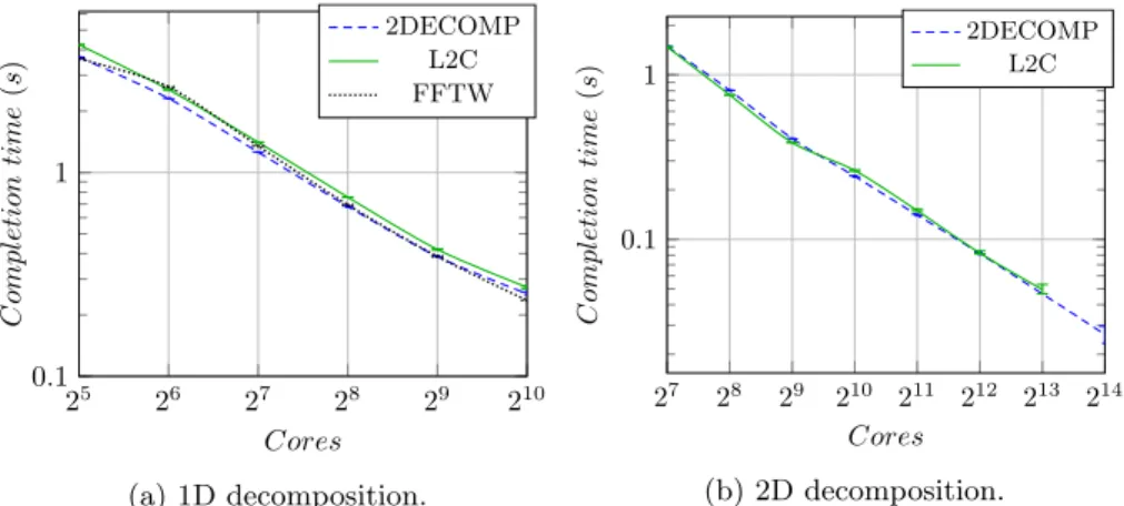
25 26 27 28 29 210 0.1 1 Cores C ompl etion time (s ) 2DECOMP L2C FFTW (a) 1D decomposition. 27 28 29 210 211 212 213 214 0.1 1 Cores C ompl etion time (s ) 2DECOMP L2C (b) 2D decomposition.
Fig. 3: Completion time of 10243complex-to-complex homogeneous 3D-FFT on
Curie using both 1D (a) and 2D decompositions (b).
Variability experiments were done on 5 clusters of the Grid’5000 experimental platform [9]: Griffon1, Graphene2, Edel3, Genepi4 and Sol5. Performance and
scalability experiments were done on thin nodes of the Curie supercomputer6.
Each experiment has been done 100 times and the median is displayed. Error bars on plots correspond to the first and last quartile.
All experiments involve complex-to-complex 3D-FFTs and use a minimum number of transpositions (i.e., 1 with 1D decomposition, 2 with 2D decompo-sition). The FFT libraries used as reference are FFTW 3.3.4 and 2DECOMP 1.5. All libraries are configured to use a synchronous complex-to-complex 3D-FFT using 3D-FFTW sequential implementation (with 3D-FFTW MEASURE planning) and double precision floating point.
5.1 Performance and Scalability Evaluation
Figure 3 displays the completion time obtained for matrices of size 10243 on
the Curie thin nodes for a 1D decomposition (Figure 3a) and 2D decomposition (Figure 3b). Overall, the performance of L2C assemblies, FFTW and 2DECOMP
are close with both 1D and 2D decomposition. With 1D decomposition, we note that L2C is slightly slower than 2DECOMP and the FFTW (up to 17%). This
gap is due to the local transposition not being optimized enough in the 3D-FFT L2C implementation (e.g., cache-use optimization). Due to the lack of 2D
decomposition support of the FFTW, this library does not appear on Figure 3b.
1 92 nodes, 2 CPU/node, 4 cores/CPU, Xeon L5420 (2.5 GHz), 20G InfiniBand 2 144 nodes, 1 CPU/node, 4 cores/CPU, Xeon X3440 (2.53 GHz), 20G InfiniBand 3 34 nodes, 2 CPU/node, 4 cores/CPU, Xeon E5520 (2.27 GHz), 40G InfiniBand 4 72 nodes, 2 CPU/node, 4 cores/CPU, Xeon E5420 QC (2.5 GHz), 40G InfiniBand 5 50 nodes, 2 CPU/node, 2 cores/CPU, AMD Opteron 2218 (2.6 GHz), 1G Ethernet 6 5040 nodes, 2 CPU/node, 8 cores/CPU, Xeon E5-2680 (2.7 GHz), 40G InfiniBand
20 21 22 23 24 25 26 27 28 0.01 0.1 1 Cores C ompl etion time (s ) 2DECOMP L2C
Fig. 4: Completion time of 2563
complex-to-complex heterogeneous 3D-FFT on Edel and Genepi using 2D decomposition.
Version C++ LOC Reused code 1D-hm-2t-naive 944 -1D-hm-2t-opt 1041 69% 1D-hm-1t 932 77% 1D-ht-2t 1101 71% 1D-ht-1t 985 80% 2D-hm-2t 1100 86% 2D-ht-2t 1150 68% 2D-ht-4t 1150 100%
Fig. 5: Number of lines of code (LOC) for several versions of the 3D-FFT application. hm: homo-geneous; ht: heterohomo-geneous; nt: n transpositions.
With 2D decomposition, the gap between 2DECOMP and L2C is lower (less
than 8%). This is a very good result as 3D-FFT L2C implementations have been
done in some weeks, and therefore they are not highly optimized. The results also show that L2C scales well up to 8,192 cores on 2D decomposition. Beyond
this limit, the L2C deployment phase has yet to be optimized to support it.
5.2 Adaptation and Reuse Evaluation
Heterogeneous Experiments Figure 4 shows the completion times obtained for matrices of size 2563 on the clusters Edel and Genepi up to 256 cores for a
2D decomposition (Figure 4). Orange area corresponds to the homogeneous case because only one Edel 8-core node is used. From 16 cores and up, half the cores are from Edel nodes and the other half from Genepi nodes. The Edel cluster is overall faster than the Genepi cluster.
We observe that from 8 to 16 nodes 2DECOMP performance decreases and L2C performance improves. That is because 2DECOMP does not balance its load and is thus limited by the speed of the slowest cluster. It means the heterogeneous L2C assembly successfully takes advantage of both clusters and is not limited by
the speed of the slowest one.
Reuse Table 5 displays code reuse (in terms of number of C++ lines) between some of the L2C assemblies. Reuse is the amount of code that is reused from the
assemblies listed higher in the table. Version code names are decomposition type (1D or 2D), followed by hm for homogeneous assemblies or ht for heterogeneous assemblies, and end with nt where n is the number of transpositions used.
We observe a high code reuse between specialized assemblies: from 68% to 100% without any low-level modification. Also note that our L2C
implementa-tions are much smaller than 2DECOMP (11,570 lines of FORTRAN code); that is also because 2DECOMP implements more features.
Since our components are medium-grained and they have simple interfaces (see Section 4), modifying an assembly for one processing element is only a mat-ter of changing a few paramemat-ters, connections and adding/removing instances. This process involves no low-level code modification. It is done at architecture level and is independent of possible changes in the component implementations. Thus, components ease the integration of new or unique optimizations.
Discussion Performance results show that L2C assemblies scale up to 8,192
cores with performance comparable to the reference libraries on Curie using 1D/2D decompositions. Adaptation results show that components help to ease implementation of new optimizations and help to combine them. Several spe-cialized assemblies have been written with high code reuse (from 68% to 100% reused code without any low-level modification). Specialization (e.g., heteroge-neous case) is often achieved using simple assembly transformations.
6
Conclusion and Future Work
To achieve adaptability of high-performance computing applications on various hardware architectures, this paper has evaluated the use of component models to handle HPC application variability. A 3D-FFT use case has been evaluated. 3D-FFT algorithms have been modelled and specialized using component models features (component replacement, attribute tuning, and assemblies). The same work could be applied on other HPC applications to ease their adaptations.
The experimental results obtained on Grid’5000 clusters and on the Curie su-percomputer show that 3D-FFT L2C assemblies can be competitive with existing
libraries in multiple cases using 1D and 2D decompositions. It is consistent with previous results obtained on a simpler use case [4]. So, using an HPC-oriented component model adds a negligible overhead while providing better software en-gineering features. Adaptation results show that performance of libraries can be increased in some special cases (e.g., heterogeneous cases) by adapting assem-blies. Re-usability results show that components enable the writing of specialized applications by reusing parts of other versions.
Results are encouraging even though more work on the L2C implementation
is needed to let it scale to at least tens of thousands of nodes. Moreover, assembly descriptions need to be rewritten for each specific hardware. As this process is fastidious and error-prone, such descriptions should be automatically generated to ease assembly building.
Possible future works include working on automating assembly generation to ease maintenance and development of assemblies by using a high-level compo-nent model which offers this possibility. One such model is HLCM [5] developed in the Avalon team. Finally, adding parameter tuning on top of high-level as-sembly would allow auto-tuning for efficient automatic generation of low-level assemblies.
References
1. Ansel, J., Chan, C., Wong, Y.L., Olszewski, M., Zhao, Q., Edelman, A., Amaras-inghe, S.: PetaBricks: a language and compiler for algorithmic choice, vol. 44. ACM (2009)
2. Baude, F., Caromel, D., Dalmasso, C., Danelutto, M., Getov, V., Henrio, L., P´erez, C.: GCM: a grid extension to Fractal for autonomous distributed components. Annales des T´el´ecommunications 64(1-2), 5–24 (2009)
3. Bernholdt, D.E., Allan, B.A., Armstrong, R., Bertrand, F., Chiu, K., Dahlgren, T.L., Damevski, K., Elwasif, W.R., Epperly, T.G., Govindaraju, M., et al.: A Component Architecture for High Performance Scientific Computing. International Journal of High Performance Computing Applications (May 2006)
4. Bigot, J., Hou, Z., P´erez, C., Pichon, V.: A low level component model easing performance portability of HPC applications. Computing (Nov 2013), http://hal.inria.fr/hal-00911231
5. Bigot, J., P´erez, C.: High Performance Composition Operators in Component Models. In: High Performance Computing: From Grids and Clouds to Exas-cale, Advances in Parallel Computing, vol. 20, pp. 182 – 201. IOS Press (2011), http://hal.inria.fr/hal-00692584
6. Boldt, J.: The Common Object Request Broker: Architecture and Specification (July 1995), http://www.omg.org/cgi-bin/doc?formal/97-02-25
7. Bonelli, A., Franchetti, F., Lorenz, J., P¨uschel, M., Ueberhuber, C.W.: Automatic Performance Optimization of the Discrete Fourier Transform on Distributed Mem-ory Computers. In: International Symposium on Parallel and Distributed Process-ing and Application (ISPA). Lecture Notes In Computer Science, vol. 4330, pp. 818–832. Springer (2006)
8. Bozga, M., Jaber, M., Sifakis, J.: Source-to-Source Architecture Transformation for Performance Optimization in BIP. Industrial Informatics, IEEE Transactions on 6(4), 708–718 (Nov 2010)
9. Desprez, F., Fox, G., Jeannot, E., Keahey, K., Kozuch, M., Margery, D., Neyron, P., Nussbaum, L., P´erez, C., Richard, O., Smith, W., Von Laszewski, G., V¨ockler, J.: Supporting Experimental Computer Science. Rapport de recherche RR-8035, INRIA (Jul 2012), http://hal.inria.fr/hal-00722605
10. Frigo, M., Johnson, S.: The Design and Implementation of FFTW3. Proceedings of the IEEE 93(2), 216–231 (Feb 2005)
11. McIlroy, M.D.: Mass-produced Software Components. Proc. NATO Conf. on Soft-ware Engineering, Garmisch, Germany (1968)
12. Pekurovsky, D.: P3DFFT: A Framework for Parallel Computations of Fourier Transforms in Three Dimensions. SIAM J. Scientific Computing 34(4) (2012), http://dblp.uni-trier.de/db/journals/siamsc/siamsc34.html#Pekurovsky12 13. Squyres, J.M., Lumsdaine, A.: The Component Architecture of Open MPI:
En-abling Third-Party Collective Algorithms. In: Component Models and Systems for Grid Applications, pp. 167–185. Springer (2005)
14. Szyperski, C.: Component Software: Beyond Object-Oriented Programming. Addison-Wesley Longman Publishing Co., Inc., Boston, MA, USA, 2nd edition edn. (2002)
15. Wang, N., Parameswaran, K., Kircher, M., Schmidt, D.C.: Applying Reflective Middleware Techniques to Optimize a QoS-Enabled CORBA Component Model Implementation. In: COMPSAC. pp. 492–499. IEEE Computer Society (2000), http://dblp.uni-trier.de/db/conf/compsac/compsac2000.html#WangPKS00