HAL Id: hal-02926464
https://hal.inria.fr/hal-02926464
Submitted on 31 Aug 2020
HAL is a multi-disciplinary open access
archive for the deposit and dissemination of
sci-entific research documents, whether they are
pub-lished or not. The documents may come from
teaching and research institutions in France or
abroad, or from public or private research centers.
L’archive ouverte pluridisciplinaire HAL, est
destinée au dépôt et à la diffusion de documents
scientifiques de niveau recherche, publiés ou non,
émanant des établissements d’enseignement et de
recherche français ou étrangers, des laboratoires
publics ou privés.
Scalable Joint Optimization of Placement and
Parallelism of Data Stream Processing Applications on
Cloud-Edge Infrastructure
Felipe Rodrigo de Souza, Alexandre da Silva Veith, Marcos Dias de Assuncao,
Eddy Caron
To cite this version:
Felipe Rodrigo de Souza, Alexandre da Silva Veith, Marcos Dias de Assuncao, Eddy Caron. Scalable
Joint Optimization of Placement and Parallelism of Data Stream Processing Applications on
Cloud-Edge Infrastructure. ICSOC 2020 - 18th International Conference on Service Oriented Computing,
Dec 2020, Dubai, United Arab Emirates. �hal-02926464�
Parallelism of Data Stream Processing
Applications on Cloud-Edge Infrastructure
Felipe Rodrigo de Souza1, Alexandre Da Silva Veith2,
Marcos Dias de Assun¸c˜ao1, and Eddy Caron1
1 Univ Lyon, EnsL, UCBL, CNRS, Inria, LIP, F-69342, LYON Cedex 07, France
2
University of Toronto, Canada
Abstract. The Internet of Things has enabled many application sce-narios where a large number of connected devices generate unbounded streams of data, often processed by data stream processing frameworks deployed in the cloud. Edge computing enables offloading processing from the cloud and placing it close to where the data is generated, whereby re-ducing both the time to process data events and deployment costs. How-ever, edge resources are more computationally constrained than their cloud counterparts. This gives rise to two interrelated issues, namely de-ciding on the parallelism of processing tasks (a.k.a. operators) and their mapping onto available resources. In this work, we formulate the scenario of operator placement and parallelism as an optimal mixed integer lin-ear programming problem. To overcome the issue of scalability with the optimal model, we devise a resource selection technique that reduces the number of resources evaluated during placement and parallelization deci-sions. Experimental results using discrete-event simulation demonstrate that the proposed model coupled with the resource selection technique is 94% faster than solving the optimal model alone, and it produces so-lutions that are only 12% worse than the optimal, yet it performs better than state-of-the-art approaches.
Keywords: Data Stream Processing· Operator Placement · Operator
Parallelism· End-to-end Latency · Edge Computing.
1
Introduction
A Data Stream Processing (DSP) application is often structured as a directed graph whose vertices represent data sources, operators that execute a function over incoming data, and data sinks; and edges that define the data interdepen-dencies between operators [4]. DSP applications are often deployed in the cloud to explore the large number of available resources and benefit from its pay-as-you-go business model. The growth of the Internet of Things (IoT) has led to scenarios where geo-distributed resources at the edge of the network act both as data sources and actuators or consumers of processed data. Streaming all this data to a cloud through the Internet, and sometimes back, takes time and quickly becomes costly [4].
Exploration of computing resources from both the cloud and the Internet edges is called as cloud-edge infrastructure. This paradigm combines cloud, micro datacenters, and IoT devices and can minimize the impact of network communi-cation on the latency of DSP applicommuni-cations. An inherent problem, however, relies upon deciding how much and which parts of a DSP application to offload from the cloud to resources elsewhere. This problem, commonly known as operator placement and shown to be NP-Hard [2], consists in finding a set of resources to host operators while meeting the application requirements. The search space can be large depending on the size and heterogeneity of the infrastructure.
When offloading operators from the cloud, the DSP framework needs to ad-just the operators’ parallelism and hence decide how to create the number of op-erator instances to achieve a target throughput. The opop-erator placement needs to address two interrelated issues, namely deciding on the number of instances for each operator and finding the set of resources to host the instances; while guaranteeing performance metrics such as application throughput and end-to-end latency. As an additional level of complexity, the deployment of DSP appli-cations in public infrastructure, such as a cloud, incurs monetary costs, which must be considered when deciding on where to place each DSP operator and how many replicas to create.
This work describes the Cloud-Edge Stream Model (CES), an extension of an optimal Mixed Integer Linear Programming (MILP) model introduced in our previous work [16] for the problem of determining the degree of parallelism and placement of DSP applications onto cloud-edge infrastructure. The model is enhanced with a heuristic that improves its scalability. We devise a solution for estimating the number of replicas, and the processing and bandwidth re-quirements of each operator to respect a given throughput and minimize the application end-to-end latency and deployment costs. The contributions of this work are therefore: (i) it presents a MILP model for the joint-optimization of operator parallelism and placement on cloud-edge infrastructure to minimize the data transfer time and the application deployment costs (§2); (ii) it introduces a resource selection technique to improve the system scalability (§3); and (iii) it evaluates the model and the resource selection technique against traditional and state-of-the-art solutions (§4).
2
Proposed Model
This section introduces preliminaries, the placement problem and CES.
2.1 System Model
This work considers a three-layered cloud-edge infrastructure, as depicted in Figure 1, where each layer contains multiple sites. The IoT layer contains nu-merous geo-distributed computational constrained resources, therefore, often acting as source or sinks, but with non negligible computational capacity to support some DSP operators. Micro Datacenters (MDs) provide geo-distributed
resources (e.g., routers, gateways, and micro datacenters), but with less strin-gent computational constraints than those in the IoT layer. The cloud comprises high-end servers with fewer resource constraints [13].
...
IoT Sites Private Infrastructure Public Infrastructure Micro Datacenters Cloud Sites ... ... ... ... ... ...Fig. 1. Target infrastructure. The three-layered cloud-edge
infrastruc-ture is represented as a graph GI = hR, Pi,
where R is the set of computing resources of all layers (RIoT ∪ RM D ∪ Rcloud), and
P is the set of network interconnections be-tween computing resources. Each k ∈ R has CPU (CP Uk) and memory (M emk)
capaci-ties, given respectively in 100×num of cores, and bytes. The processing speed of a resource (Vk) is its CPU clock in GHz. Similar to
exist-ing work [9], the network has a sexist-ingle intercon-nection between a pair of computing resources k and l, and the bandwidth of this intercon-nection is given by Bwk,l and its latency is Latk,l.
The application graph specified by a user is a directed graph GA = hO, E i,
where O represents data source(s) SourceO, data sink(s) SinkO and transforma-tion operators T ransO, and E represents the streams between operators, which are unbounded sequences of data (e.g., messages, packets, tuples, file chunks) [4]. The application graph contains at least one data source and one data sink. Each operator j ∈ O is the tuple hSj, Cj, Uj, ARji, where Sj is the selectivity
(mes-sage discarding percentage), Cj is the data transformation factor (how much it increases/decreases the size of arriving messages), Uj is the set of upstream operators directly connected to j, and ARj is the input rate in Bps that arrives at the operator. When operator j is a data source (i.e., j ∈ SourceO) its input rate is the amount of data ingested into the application since Uj= ∅. Otherwise, ARj is recursively computed as:
ARj = X
i∈Uj
ρi→j× DRi (1)
where ρi→j is the probability that operator i will send an output message to
operator j, capturing how operator i distributes its output stream among its downstream operators. DRi is the departure rate of operator i after applying
selectivity Si and the data transformation factor Ci to the input stream:
DRi= ARi× (1 − Si) × Ci (2)
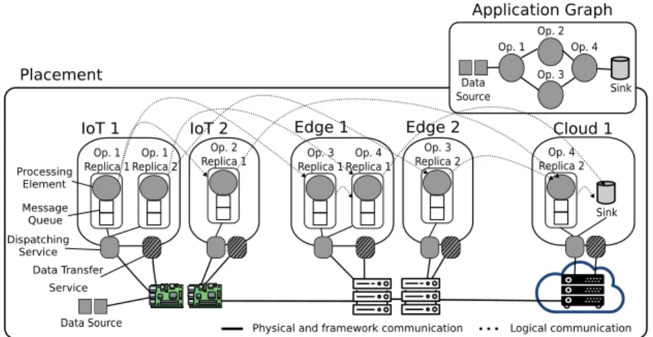
A physical representation of the application graph is created when operators are placed onto available resources as depicted in Figure 2. Operators placed within the same host communicate directly whereas inter-resource communica-tion is done via the Data Transfer Service. Messages that arrive at a computing resource are received by the Dispatching Service, which then forwards them to the destination operator within the computing resource. This service also passes messages to the Data Transfer Service when inter-resource communication is
required. Each operator comprises an internal queue and a processing element, which are treated as a single software unit when determining the operator prop-erties (e.g., selectivity and data transformation factor), and its CPU and memory requirements. Moreover, an operator may demand more CPU than what a single resource can offer. In this case, multiple operator replicas are created in a way that each individual replica fits a computing resource.
Physical and framework communication Logical communication
IoT 1 Message Queue IoT 2 Data Transfer Service Dispatching Service Data Source Placement Sink Data Source Op. 1 Op. 2 Op. 3 Op. 4 Op. 4 Replica 1 Op. 3 Replica 1 Op. 3 Replica 2 Op. 1 Replica 2 Op. 1 Replica 1 Op. 2
Replica 1 Replica 2Op. 4 Sink
Edge 1 Edge 2 Cloud 1
Processing Element
Application Graph
Fig. 2. Application graph adjusted to the computing resource capacities (placement). The quality of a placement is guaranteed by meeting the application require-ments. The CPU and memory requirements of each operator j for processing its incoming byte stream are expressed as Reqj
cpuand Reqjmemand they are
ob-tained by profiling the operator on a reference resource [1]. Refj
cpu, Refmemj and
Refdataj refers to the reference CPU, memory and processed data of operator j, respectively. Since CPU and memory cannot be freely fractioned, the reference values are rounded up and combined with ARj of j in order to compute Reqjcpu
and Reqj
mem that handle the arriving data stream:
Reqcpuj = & Refj cpu× ARj Refdataj '
and Reqmemj = & Refj mem× ARj Refdataj ' (3) 2.2 Problem Formulation
The problem is modeled as a MILP with variables x(j, l) and f (i, k → j, l). Variable x(j, l) accounts for the amount of bytes that a replica of operator j can process on resource l, whereas variable f (i, k → j, l) corresponds to the number of bytes that operator replica i on resource k sends to downstream operator replica j deployed on resource l.
The data ingestion rate in sources is constant and stable. Hence, it is possible to compute CPU and memory requirements recursively to the entire application
to handle the expected load. Placing an application onto computing resources incurs a cost. This cost is derived from Amazon Fargate’s pricing scheme3.The
cost of using one unit of CPU and storing one byte in memory at resource l is given by Ccpu(l) and Cmem(l), respectively. While the cost of transferring a byte
over the network from resource k to l is denoted by Cbw(k, l).
As cloud-edge infrastructure comprises heterogeneous resources, the model applies a coefficient Ωl = RefVj/Vl to adapt the operator requirements to
re-source l. RefVj is the reference processing speed of the resource for operator j, and Vlis the clock speed of resource l. The computational cost is given by:
CC =X l∈R X j∈O Ccpu(l) × Reqcpuj Ωl ×β×x(j,l) ARj max Ccpu(l) +Cmem(l) × Reqj mem×x(j,l) ARj max Cmem(l) (4)
where max Ccpu(l) and max Cmem(l) are the cost of using all the CPU and
memory capacity of resource l. The CPU and memory costs are normalized using their maximum amounts resulting in values between 0 and 1. β refers to a safety margin to each replica requirements aiming to a steady safe system. This margin relies on Queueing Theory premises to avoid an operator reaching the CPU limits of a given computing resource, which requires a higher queuing time.
The network cost N C is computed as: N C =X p∈P X a,b∈p X j∈O X i∈Uj Cbw(a, b) × f (i, ps→ j, pd) max Cbw(a, b) (5)
where a, b is a link that represents one hop of path p, and a, b can belong to multiple paths. The resources at the extremities of path p hosting replicas i and j are given by ps and pd, respectively. N C is normalized by max Cbw(a, b), the
cost of using all the bandwidth available between resources a and b.
The Aggregate Data Transfer Time (ATT) sums up the network latency of a link and the time to transfer all the data crossing it, and is normalized by the time it takes to send an amount of data that fills up the link capacity:
AT T =X p∈P X k,l∈p X j∈O X i∈Uj f (i, ps→ j, pd) × (Latk,l+Bw1k,l) Latk,l+ 1 (6)
The multi-objective function aims at minimizing the data transfer time and the application deployment costs:
min : AT T + CC + N C (7)
The objective function is subject to:
Physical constraints: The requirements of each operator replica j on re-source l are a function of x(j, l); i.e., a fraction of the byte rate operator j
3
should process (ARj) with a safety margin (β). The processing requirements of
all replicas deployed on l must not exceed its processing capacity, as follows:
CP Ul≥ X j∈O Reqcpuj Ωl × β × x(j, l) ARj and M eml≥ X j∈O Reqj mem× x(j, l) ARj (8)
To guarantee that the amount of data crossing every link a, b must not exceed its bandwidth capacity:
X
j∈O
X
i∈Uj
f (i, ps→ j, pd) ≤ Bwa,b ∀a, b ∈ p; ∀p ∈ P (9)
Processing constraint: The amount of data processed by all replicas of j must be equal to the byte arrival rate of j:
ARj=X
l∈R
x(j, l) ∀j ∈ O (10)
Flow constraints: Except for sources and sinks, it is possible to create one replica of operator j per resource, although the actual number of replicas, the processing requirements, and the interconnecting streams are decided within the model. The amount of data that flows from all replicas of i to all the replicas of j is equal to the departure rate of upstream i to j:
DRi× ρi→j= X
k∈R
X
l∈R
f (i, k → j, l) ∀j ∈ O; ∀i ∈ Uj (11)
Likewise, the amount of data flowing from one replica of i can be distributed among all replicas of j:
x(i, k) × (1 − Si) × Ci× ρi→j =X
l∈R
f (i, k → j, l) ∀k ∈ R; ∀j ∈ O; ∀i ∈ Uj
(12)
On the other end of the flow, the amount of data arriving at each replica j of operator i, must be equal to the amount of data processed in x(j, l):
X
i∈Uj
X
k∈R
f (i, k → j, l) = x(j, l) ∀j ∈ O; ∀l ∈ R (13)
Domain constraints: The placement k of sources and sinks is fixed and pro-vided in the deployment requirements. Variables x(j, l) and f (i, k → j, l) repre-sent respectively the amount of data processed by j in l, and the amount of data sent by replica i in k to replica j in l. Therefore the domain of these variables is a real value greater than zero:
x(j, l) = ARj ∀j ∈ SourceO∪ SinkO; ∀l ∈ R (14) x(j, l) ≥ 0 ∀j ∈ T ransO; ∀l ∈ R (15) f (i, k → j, l) ≥ 0 ∀k, l ∈ R; j ∈ O; i ∈ Uj (16)
3
Resource Selection Technique
The three-layered cloud-edge infrastructure may contain thousands of computing resources resulting in an enormous combinatorial search space when finding an optimal operator placement. This work therefore proposes a pruning technique that reduces the number of evaluated resources and finds a sub-optimal solution under feasible time. The proposed solution extends the worst fit sorting heuristic from Taneja et al. [17] by applying a resource selection technique to reduce the number of considered computing resources when deploying operators.
The resource selection technique starts by identifying promising sites in each layer from which to obtain computing resources. Following a bottom-up ap-proach, it selects all IoT sites where data sources and data sinks are placed. Then, based on the location of the selected IoT sites, it picks the MD site with the shortest latency to each IoT site plus the MD sites where there are data sources and data sinks placed. Last, the cloud sites are chosen considering their latency-closeness to the selected MD sites as well as those with data sources and data sinks. After selecting sites from each layer, the function GetResources (Algorithm 1) is called for each layer.
As depicted in Algorithm 1, GetResources has as input the layer name, the vector of selected sites in the layer and the set of operators. First, it calls GetResourcesOnSites, to get all computing resources from the selected sites, sorted by CPU and memory in a worst-fit fashion (line 3). Second, it selects resources that host sources or sinks (lines 4-7). Third, CPU and memory re-quirements from the operators that are neither sources or sinks are summed to ReqCP U and ReqM em, respectively (line 9). When the evaluated layer is IoT, ReqCP U and ReqM em are used to select a subset of computing resources whose combined capacity meets the requirements (lines 18-21). For each operator of the other two layers, the function selects a worst-fit resource that supports the operator requirements. Since the goal is just to select candidate resources and not a deployment placement, if there is no resource fit, it ignores the operator and moves to the next one (lines 11-16). At last, the combination of resources evaluated by the model contains those selected in each layer.
4
Performance Evaluation
This section describes the experimental setup, the price model for computing resources, and performance evaluation results.
4.1 Experimental Setup
We perform an evaluation in two steps as follows. First CES is compared against a combination of itself with the resource selection technique, hereafter called CES-RS, to evaluate the effects that the resource pruning has on the quality of solutions and on resolution time. Second, we compare CES-RS against state-of-the-art solutions. The evaluations differ in the number of resources in the
Algorithm 1: Resource selection technique.
1 Function GetResources(layer, Sites, O)
2 Selected ← {}, ReqCP U ← 0, ReqM em ← 0
3 Resources ← GetResourcesOnSites (Sites)
4 foreach j ∈ (SourceO∪ SinkO
) do
5 if j.placement ∈ Resources then
6 Selected ← Selected ∪ j.placement
7 Resources ← Resources − j.placement
8 foreach j ∈ (O − (SourceO∪ SinkO
)) do
9 ReqCP U ← ReqCP U + CP Uj, ReqM em ← ReqM em + M emj
10 if layer! = IoT then
11 foreach r ∈ Resources do 12 if CP Ur≥ CP Ujand M emr ≥ M emjthen 13 selected ← selected ∪ r 14 Resources ← Resources − r 15 break 16 Sort (Resources)
17 if layer == IoT then
18 foreach r ∈ Resources do
19 if CP Ur≤ ReqCP U or M emr≤ ReqM em then
20 Selected ← Selected ∪ r
21 ReqCP U ← ReqCP U − CP Ur, ReqM em ← ReqM em − M emr
22 else
23 break
24 return Selected
infrastructure and the solutions evaluated. Both evaluations are performed via discrete-event simulation using a framework built on OMNET++ to model and simulate DSP applications. We resort to simulation as it offers a controllable and repeatable environment. The model is solved using CPLEX v12.9.0.
The infrastructure comprises three layers with an IoT site, one MD and one cloud. The resource capacity was modeled according to the characteristics of the layer in which a resource is located, and intrinsic characteristics of DSP appli-cations. IoT resources are modeled as Raspberry Pi’s 3 (i.e., 1 GB of RAM, 4 CPU cores at 1,2 GHz). As DSP applications are often CPU and memory inten-sive, the selected MD and cloud resources should be optimized for such cases. The offerings for MD infrastructure are still fairly recent and, although there is a lack of consensus surrounding what the MD is composed of, existing work highlights that the options are more limited than those of the cloud, with more general-purpose resources. In an attempt to use resources similar to those avail-able on Amazon EC2, MD resources are modeled as general purpose t2.2xlarge machines (i.e., 32 GB of RAM, 8 CPU cores at 3.0 GHz), and cloud servers are high-performance C5.metal machines (i.e., 192 GB of RAM, 96 CPU cores at
3.6 GHz). Resources within a site communicate via a LAN, whereas IoTs, MDs, and cloud are interconnected by single WAN path. The LAN has a bandwidth of 100 Mbps and 0.8 ms latency. The WAN bandwidth is 10 Gbps and is shared on the path from the IoT to the MD or to the cloud, and the latency from IoT is 20 ms and 90 ms to the MD and cloud, respectively. The latency values are based on those obtained by empirical experiments carried out by Hu et. al [9].
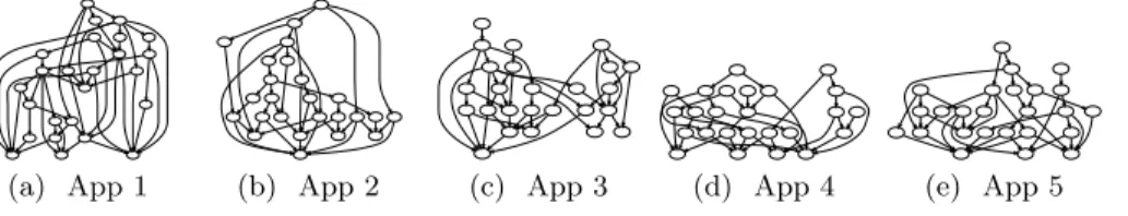
Existing work evaluated application graphs of several orders and intercon-nection probabilities, usually assessing up to 3 different graphs [4, 7, 8, 10]. To evaluate CES and CES-RS we crafted five graphs to mimic the behaviour of large DSP applications using a built-in-house python library. The graphs have varying shapes and data replication factors for each operator as depicted in Fig. 3. The applications have 25 operators, often more than what is considered in the liter-ature [18]. They also have multiple sources, sinks and paths, similar to previous work by Liu and Buyya [10]. As the present work focuses on IoT scenarios, the sources are placed on IoT resources, and sinks are uniformly and randomly dis-tributed across layers as they can be actuators – except for one sink responsible for data storage, which is placed on the cloud.
(a) App 1 (b) App 2 (c) App 3 (d) App 4 (e) App 5
Fig. 3. Application graphs used in the evaluation.
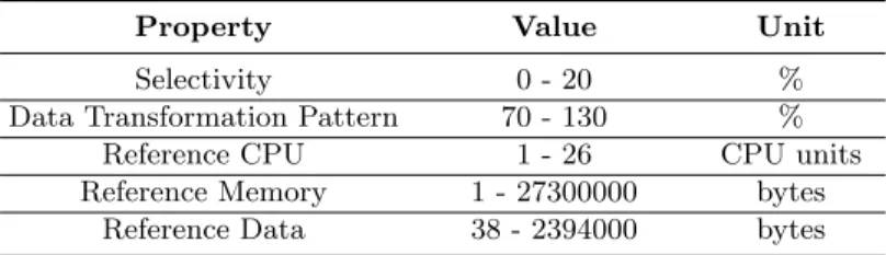
The operator properties were based on the RIoTBench IoT application bench-mark [15]. RIoTBench offers 27 operators common to IoT applications and 4 datasets with IoT data. The CITY dataset is used with 380 byte messages col-lected every 12 seconds containing environmental information (temperature, hu-midity, air quality) from 7 cities across 3 continents. It has a peak rate of 5000 tuples/s, which in the experiments is continuous and divided among sources. The remaining properties are drawn from the values in Table 1.
We consider that Refj cpu, Ref
j
data, the arrival byte rate AR
j, probability
that an upstream operator i sends data to j ρi→j, selectivity Sj, and data transformation pattern Cj, are average values obtained via application profiling, using techniques proposed in existing work [1]. With Refcpuj and Ref
j
datawe are
able to compute requirements for each operator To create a worst case scenario in terms of load, ρi→jis set to 1 for all streams in the application request. As the
model creates multiple replicas, ρi→j gets divided among instances of operator
j, hence creating variations on the arrival rate of downstream operators during runtime. The operator processing requirements estimated by the model may not be enough to handle the actual load during certain periods, so resulting in large operator queues. To circumvent this issue we add a small safety margin, the β factor, as mentioned in Section 2.2, which is a percentage increase in the
Table 1. Operator properties in the application graphs.
Property Value Unit
Selectivity 0 - 20 %
Data Transformation Pattern 70 - 130 %
Reference CPU 1 - 26 CPU units
Reference Memory 1 - 27300000 bytes
Reference Data 38 - 2394000 bytes
application requirements estimated by the proposed model. A β too high results in expensive over-provisioning. After multiple empirical evaluations, β was set to 10% of each replica requirement.
Price model: The price of using resources is derived from Amazon AWS ser-vices, considering the US East Virginia location. The CPU and memory prices are computed based on the AWS Fargate Pricing4 under a 24/7 execution.
Re-garding the network, we consider a Direct Connection5 between the IoT site
and the AWS infrastructure. Direct Connections are offered under two options, 1 GB/s and 10 GB/s. As DSP applications generate large amounts of data, we consider the 10 GB/s offer. The data sent from the IoT to AWS infrastructure uses AWS IoT Core6. Connections between operators on the edge or on IoT
resources to the cloud use Private Links7. Amazon provides the values for CPU,
memory and network as, respectively, fraction of a vCPU, GB and Gbps, but in our formulation the values for the same metrics are computed in CPU units (100 ∗ num cores), bytes and Mbps. The values provided by Amazon converted to the scale used in our formulation are presented in Table 2. As the environment combines both public and private infrastructure, deployment costs are applied only to MD and cloud resources, the network between these two, and the network between these two and IoT resources. As IoT resources are on the same private network infrastructure, the communication between IoT resources is free.
Evaluated approaches and metrics: Five different configurations of de-ployment requests are submitted for each application. The reported values for each application are averages of these five executions. Each deployment request has a different placement for sources and sinks with sources always on IoT re-sources and at least one sink in the cloud. The operator properties such as selectivity and data transformation pattern vary across configurations.
The performance of DSP applications is usually measured considering two main metrics, namely throughput, which is the processing rate, in bytes/s, of all sinks in the application; and end-to-end latency, which is the average time span from when a message is generated until it reaches a sink. The MILP model
4 https://aws.amazon.com/fargate/ 5 https://aws.amazon.com/directconnect/ 6 https://aws.amazon.com/iot-core/ 7 https://aws.amazon.com/privatelink/
Table 2. Computing and network costs.
Resource Unit Cost
CPU CPU/month $0.291456
Memory byte/month $3.2004e-09
Direct Link IoT to AWS 10GB link/Month $1620
Link IoT to AWS Connection/Month $0.003456
KB $0.0000002
Communication IoT to cloud,
GB $7.2 + 0.01 per GB
IoT to MD, and MD to cloud
takes the throughput into account in the constraints, and the end-to-end latency indirectly by optimizing the Aggregate Data Transfer Time.
4.2 Resolution Time versus Solution Quality
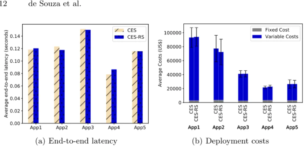
Here we evaluate how much the quality of a solution is sacrificed by reducing the search space. The simulation, which runs for 220 seconds, considers 100 IoT devices, a MD with 50 resources and a cloud with 50 resources. The throughput is the same in all scenarios since it is guaranteed as a model constraint.
Figure 4 shows the end-to-end latency and deployment costs under CES and CES-RS. There are some variations regarding the end-to-end latency both on CES and on CES-RS. Since CES-RS aims to reduce the search space, it might be counter intuitive to see cases where the resource selection with less options obtains better end-to-end latency, such as in App3. However, the objective func-tion considers both latency and execufunc-tion costs as optimisafunc-tion metrics. As CES searches to strike a balance between cost and end-to-end latency, the average deployment costs obtained with CES-RS for App 3 (Figure 4(b)) are higher. This behavior happens because under the limited search space, CES-RS finds sub-optimal solutions, where the best trade-off resulted in better end-to-end la-tency. To do so, it needed to use more edge or cloud devices, which incurs higher computational and network costs.
As CES considers the whole search space, it explores more options and yields better results. Despite reduced search space CES-RS can produce very similar results – in the worst case yielding an end-to-end latency ' 12% worse, and deployment costs ' 12% higher. The resolution time (Figure 5), clearly shows that CES considering the whole infrastructure faces scalability issues. Despite producing results that sometimes are worse than those achieved under CES, CES-RS can obtain a solution up to ' 94% faster. CES-RS would yield even more similar results on a larger infrastructure because their search space is limited by the application size and requirements rather then by the infrastructure size. 4.3 Comparing CES-RS Against the State-of-the-Art
CES-RS is compared against two state-of-the-art approaches, namely Cloud-Only and Taneja’s Cloud-Edge Placement (TCEP). Cloud-Only applies a random walk
App1 App2 App3 App4 App5 0.00 0.02 0.04 0.06 0.08 0.10 0.12 0.14
Average end-to-end latency (seconds)
CES CES-RS
(a) End-to-end latency
CES App1CES-RS App1 CES App2CES-RS App2 CES App3CES-RS App3 CES App4CES-RS App4 CES App5CES-RS App5 0 20000 40000 60000 80000 100000
Average Costs (US$)
Fixed Cost Variable Costs
(b) Deployment costs Fig. 4. End-to-end latency and deployment costs under CES and CES-RS.
CES App1CES-RS CES App2CES-RS CES App3CES-RS CES App4CES-RS CES App5CES-RS 0 10 20 30 40
Solution Time (seconds)
Fig. 5. Resolution time to obtain a deployment solution.
considering only cloud resources, and TCEP is the work proposed by Taneja et al. [17], where all resources (IoT, MD and cloud) are sorted accordingly with their capacities, and for each operator it s elects a resource from the middle of the sorted list. This experiment was executed during 120 seconds and considered 400 IoT devices, 100 resources on the MD and 100 resources on the cloud.
Figure 6 shows the throughput and end-to-end latency for all solutions, with averages for each application. Since CES-RS guarantees a maximum throughput through a constraint, on the best case the other approaches would achieve the same values, and this can be observed on App3, App4 and App5. But under App1 and App2 Cloud-Only struggles because these applications perform a lot of data replication, thus producing large volumes of data. The large volume of messages generated by App1 and App2 has an even bigger effect on the end-to-end latency for Cloud-Only. When compared to Cloud-Only, TCEP provided better results, but still ' 80% worse than the results provided by RS. CES-RS achieves low values because, different from Cloud-Only and TCEP, it creates several replicas, being able to better explore the IoT resources considering their computational capacities and even further reducing the amount of data that is send through the internet, facing less network congestion.
App1 App2 App3 App4 App5 0 5 10 15 20 25 30 Average Throughput (Mbps) Cloud-Only TCEP CES-RS (a) Throughput
App1 App2 App3 App4 App5
102
103
104
Average end-to-end latency (ms)
Cloud-Only TCEP CES-RS
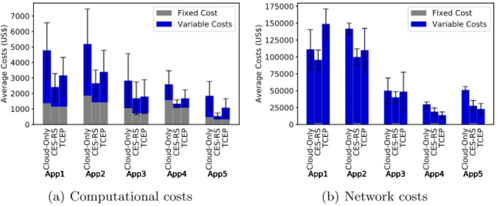
(b) End-to-end latency Fig. 6. Throughput and latency under CES-RS and state-of-the-art solutions. Figure 7 contains the costs results. Beyond better end-to-end latency, CES-RS provides better computational costs. The reason that makes CES-CES-RS achieve computational costs at least ' 6% better than the traditional approaches is the creation of replicas. The considered cost model, accounts for an IoT infrastruc-ture without deployment costs, making such devices very attractive for deploy-ment. Since IoT devices have constrained computational capacity, it is hard to deploy on such devices. Due to CES, CES-RS breaks an operator into several small replicas, allowing the use of IoT resources.
Regarding network costs, CES-RS provides cheaper deployments on most cases except on App4 and App5. In these two applications, IoT resources support the operators’ requirements without creating operator replicas allowing TCEP to exploit it and result in fewer data transfers. TCEP has higher computational costs because it cannot split operators into multiple replicas, thus resulting in placing the whole operator on powerful and expensive computing resources lo-cated on the cloud or a MD. When CES-RS is compared to TCEP, it achieves a lower computational cost and a shorter end-to-end latency.
Cloud-OnlyApp1CES-RS App1 TCEP App1 Cloud-OnlyApp2 CES-RS App2 TCEP App2 Cloud-OnlyApp3 CES-RS App3 TCEP App3 Cloud-OnlyApp4 CES-RS App4 TCEP App4 Cloud-OnlyApp5 CES-RS App5 TCEP App5 0 1000 2000 3000 4000 5000 6000 7000
Average Costs (US$)
Fixed Cost Variable Costs
(a) Computational costs
Cloud-OnlyApp1CES-RS App1 TCEP App1 Cloud-OnlyApp2 CES-RS App2 TCEP App2 Cloud-OnlyApp3 CES-RS App3 TCEP App3 Cloud-OnlyApp4 CES-RS App4 TCEP App4 Cloud-OnlyApp5 CES-RS App5 TCEP App5 0 25000 50000 75000 100000 125000 150000 175000
Average Costs (US$)
Fixed Cost Variable Costs
(b) Network costs
5
Related Work
The problem of placing DSP dataflows onto heterogeneous resources has been shown to be at least NP-Hard [2]. Moreover, most of the existing work neglects the communication overhead [6], although it is relevant in geo-distributed in-frastructure [9]. Likewise, the considered applications are often oversimplified, ignoring operator patterns such as selectivity and data transformation [14].
Effort has been made on modeling the operator placement on cloud-edge in-frastructure, including sub-optimal solutions [5,17], heuristic-based approaches [12, 19], while others focus on end-to-end latency neglecting throughput, application deployment costs, and other performance metrics when estimating the oper-ator placement [3, 4]. Existing work also explores Network Function Virtual-ization (NFV) for placing IoT application service chains across fog infrastruc-ture [11]. Solutions for profiling DSP operators are also available [1]. The present work addresses operator placement and parallelism across cloud-edge infrastruc-ture considering computing and communication constraints by modeling the sce-nario as a MILP problem and offering a solution for reducing the search space.
6
Conclusion
This work presented CES, a MILP model for the operator placement and paral-lelism of DSP applications that optimizes the end-to-end latency and deployment costs. CES combines profiling information with the computed amount of data that each operator should process whereby obtaining their processing require-ments to handle the arriving load and achieve maximum throughput. The model creates multiple lightweight replicas to offload operators from the cloud to the the edge, thus obtaining lower end-to-end latency.
To overcome the issue of scalability with CES, we devise a resource selection technique that reduces the number of resources evaluated during placement and parallelization decisions. The proposed model coupled with the resource selec-tion technique (i.e., CES-RS) is 94% faster than solving CES alone, it produces solutions that are only 12% worse than those achieved under CES and per-forms better than traditional and state-of-the-art approaches. As a future work we intent to apply the proposed model along with its heuristic to a real-world scenario.
References
1. Arkian, H., Pierre, G., Tordsson, J., Elmroth, E.: An experiment-driven perfor-mance model of stream processing operators in Fog computing environments. In: ACM/SIGAPP Symp. On Applied Computing (SAC 2019). Brno, Czech Republic (Mar 2020)
2. Benoit, A., Dobrila, A., Nicod, J.M., Philippe, L.: Scheduling linear chain streaming applications on heterogeneous systems with failures. Future Gener. Comput. Syst. 29(5), 1140–1151 (Jul 2013)
3. Canali, C., Lancellotti, R.: GASP: genetic algorithms for service placement in fog computing systems. Algorithms 12(10), 201 (2019)
4. Cardellini, V., Lo Presti, F., Nardelli, M., Russo Russo, G.: Optimal operator deployment and replication for elastic distributed data stream processing. Concur-rency and Computation: Practice and Experience 30(9), e4334 (2018)
5. Chen, W., Paik, I., Li, Z.: Cost-aware streaming workflow allocation on geo-distributed data centers. IEEE Transactions on Computers (Feb 2017)
6. Cheng, B., Papageorgiou, A., Bauer, M.: Geelytics: Enabling on-demand edge an-alytics over scoped data sources. In: IEEE Int. Cong. on BigData (2016)
7. Gedik, B., Schneider, S., Hirzel, M., Wu, K.L.: Elastic scaling for data stream processing. IEEE Tr. on Parallel and Distributed Systems 25(6), 1447–1463 (2013) 8. Hiessl, T., Karagiannis, V., Hochreiner, C., Schulte, S., Nardelli, M.: Optimal place-ment of stream processing operators in the fog. In: 2019 IEEE 3rd Int. Conf. on Fog and Edge Computing (ICFEC). pp. 1–10. IEEE (2019)
9. Hu, W., Gao, Y., Ha, K., Wang, J., Amos, B., Chen, Z., Pillai, P., Satyanarayanan, M.: Quantifying the impact of edge computing on mobile applications. In: Proc. of the 7th ACM SIGOPS Asia-Pacific Workshop on Systems. p. 5. ACM (2016) 10. Liu, X., Buyya, R.: Performance-oriented deployment of streaming applications on
cloud. IEEE Tr. on Big Data 5(1), 46–59 (March 2019)
11. Nguyen, D.T., Pham, C., Nguyen, K.K., Cheriet, M.: Placement and chaining for run-time IoT service deployment in edge-cloud. IEEE Transactions on Network and Service Management pp. 1–1 (2019)
12. Peng, Q., Xia, Y., Wang, Y., Wu, C., Luo, X., Lee, J.: Joint operator scaling and placement for distributed stream processing applications in edge computing. In: Int. Conf. on Service-Oriented Computing. pp. 461–476. Springer (2019)
13. Puthal, D., Obaidat, M.S., Nanda, P., Prasad, M., Mohanty, S.P., Zomaya, A.Y.: Secure and sustainable load balancing of edge data centers in fog computing. IEEE Communications Magazine 56(5), 60–65 (2018)
14. Sajjad, H.P., Danniswara, K., Al-Shishtawy, A., Vlassov, V.: Spanedge: Towards unifying stream processing over central and near-the-edge data centers. In: 2016 IEEE/ACM Symp. on Edge Comp. (Oct 2016)
15. Shukla, A., Chaturvedi, S., Simmhan, Y.: Riotbench: A real-time iot benchmark for distributed stream processing platforms. corr abs/1701.08530 (2017). arxiv. org/abs/1701.08530 (2017)
16. de Souza, F.R., da Silva Veith, A., Dias de Assun¸c˜ao, M., Caron, E.: An optimal model for optimizing the placement and parallelism of data stream processing applications on cloud-edge computing. In: 32nd IEEE Int. Symp. on Computer Architecture and High Performance Computing. IEEE (2020), in press
17. Taneja, M., Davy, A.: Resource aware placement of iot application modules in fog-cloud computing paradigm. In: IFIP/IEEE Symp. on Integrated Net. and Service Mgmt (IM) (May 2017)
18. Zeuch, S., Monte, B.D., Karimov, J., Lutz, C., Renz, M., Traub, J., Breß, S., Rabl, T., Markl, V.: Analyzing efficient stream processing on modern hardware. Proc. VLDB Endow. 12(5), 516–530 (Jan 2019)
19. Zhang, S., Liu, C., Wang, J., Yang, Z., Han, Y., Li, X.: Latency-aware deployment of iot services in a cloud-edge environment. In: Int. Conf. on Service-Oriented Computing. pp. 231–236. Springer (2019)