HAL Id: hal-01663802
https://hal.archives-ouvertes.fr/hal-01663802
Submitted on 26 Apr 2018
HAL is a multi-disciplinary open access
archive for the deposit and dissemination of
sci-entific research documents, whether they are
pub-lished or not. The documents may come from
teaching and research institutions in France or
abroad, or from public or private research centers.
L’archive ouverte pluridisciplinaire HAL, est
destinée au dépôt et à la diffusion de documents
scientifiques de niveau recherche, publiés ou non,
émanant des établissements d’enseignement et de
recherche français ou étrangers, des laboratoires
publics ou privés.
conductor and fluctuation-dissipation relation
Luca Magazzù, Davide Valenti, Bernardo Spagnolo, Thierry Martin, Giuseppe
Falci, Elisabetta Paladino
To cite this version:
Luca Magazzù, Davide Valenti, Bernardo Spagnolo, Thierry Martin, Giuseppe Falci, et al..
De-tector’s quantum backaction effects on a mesoscopic conductor and fluctuation-dissipation relation.
Fortschritte der Physik / Progress of Physics, 2017, Special Issue: International Conference Frontiers
of Quantum and Mesoscopic Thermodynamics Prague, Czech Republic 27 July– 1 August 2015, 65
(6-8), pp.1600059. �10.1002/prop.201600059�. �hal-01663802�
Detector’s quantum backaction effects on a mesoscopic
conductor and fluctuation-dissipation relation
Luca Magazzù
1,2,3, Davide Valenti
1, Bernardo Spagnolo
1,2,4, Thierry Martin
5,
Giuseppe Falci
4,6,7, and Elisabetta Paladino
4,6,7∗When measuring quantum mechanical properties of charge transport in mesoscopic conductors, backac-tion effects occur. We consider a measurement setup with an elementary quantum circuit, composed of an inductance and a capacitor, as detector of the current flowing in a nearby quantum point contact. A quantum Langevin equation for the detector variable including backaction effects is derived. Differences with the quan-tum Langevin equation obtained in linear response are pointed out. In this last case, a relation between fluc-tuations and dissipation is obtained, provided that an effective temperature of the quantum point contact is defined.
1 Introduction
Probing a quantum system implies disturbing its state according to the Heisenberg uncertainty principle. Mea-surements on a mesoscopic system require quantum de-tectors, and measurement-induced disturbances result in quantum backaction. Research on quantum electronics has progressed to the point where backaction effects, of-ten near to the limit imposed by the uncertainty relations, are of key relevance to experiments [1–5]. This is the case of nanoelectromechanical systems where quantum elec-tronic conductors have been used as position detection of nanomechanical oscillators [6–11]. Analogous backac-tion effects occur when measuring quantum mechanical properties of charge transport in mesoscopic conductors. In fact, to perform time-resolved detection of the quan-tum mechanical current in a quanquan-tum transport process, mesoscopic on-chip detectors are required. Some effects of the detector backaction have been addressed already in the literature [12–18] also in connection with qubit measurements [19–29], a relevant issue for quantum net-working [30–32]
In the present work we address the quantum
backac-tion effects of a mesoscopic detector on a prototype quan-tum conductor, a quanquan-tum point contact (QPC) consisting of two metallic leads driven out of equilibrium by a static voltage bias which establishes a tunneling current [33–35]. We model the detector as a dissipative quantum LC cir-cuit which is coupled inductively to the QPC [36–42]. In this scheme, the detector is continuously weakly coupled to the mesoscopic conductor. Measurement-induced dis-turbances on the QPC affect the detector. These are the focus of our work. We derive a Quantum Langevin Equa-tion (QLE) for the charge on the capacitor’s plates, corre-sponding to the x coordinate of the quantum oscillator, accounting for backaction effects. The QLE, derived per-turbatively in the LC-QPC coupling, presents non trivial damping and frictional terms in addition to the traditional ones entering the QLE of a dissipative quantum harmonic oscillator [43, 44]. We compare this equation with the QLE for our dissipative detector coupled to the QPC obtained in linear response. In this case the QPC’s force noise is not related to the QPC damping kernel via the temperature, as it would be for an equilibrium system [43, 45, 46], [47, and references therein]. However, similarly to other
analy-∗ Corresponding author E-mail: [email protected]
1 Dipartimento di Fisica e Chimica, Group of Interdisciplinary Theoretical Physics, Università di Palermo and CNISM, Unità di Palermo, Viale delle Scienze, Edificio 18, I-90128 Palermo, Italy
2 Radiophysics Department, Lobachevsky State University of Nizhny Novgorod, Russia
3 Institute of Physics, University of Augsburg, Univer-sitätsstrasse 1, D-86135 Augsburg, Germany
4 Istituto Nazionale di Fisica Nucleare, Sezione di Catania, Italy 5 Aix Marseille Université, Université de Toulon, CNRS, CPT,
UMR 7332, 13288 Marseille, France
6 Dipartimento di Fisica e Astronomia, Università di Catania, Via Santa Sofia 64, 95123 Catania, Italy
7 CNR-IMM UOS Università (MATIS), Consiglio Nazionale delle Ricerche, Catania, Italy
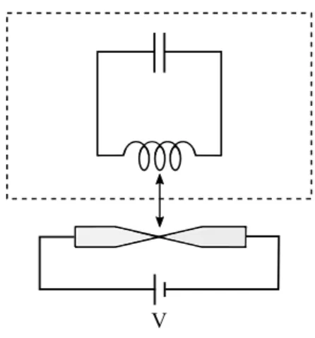
V
Figure 1 Scheme of the LC oscillator (upper part) coupled to
the quantum point contact with external biaseV = µL− µR
(lower part). The dashed box indicate the dissipative environ-ment in which the oscillator is embedded.
ses [15, 48–50], we find that, in linear response, for each given frequency, an effective temperature can be defined. In the present work, the measured system is a non-linear and non-equilibrium system. This places our work in the intriguing and timely research field investigating connec-tions among quantum measurements, fluctuaconnec-tions theo-rems and non-equilibrium systems [51–57].
The paper is organized as follows. In the next section we introduce the model. The full Hamiltonian consists of three parts, namely the dissipative resonant circuit described by the Caldeira-Leggett model, the QPC part and the inductive QPC-detector coupling. In Sec. 3 the Heisenberg equation for the QPC current including back-action contributions is solved and the full QLE is derived. Within linear response theory, we derive a QLE analogous to that found for a classical variable whose average is the expectation value of the operator x [15, 49]. In Sec. 4, a fluctuation-dissipation relation for our system, in linear response regime, is derived provided that an effective tem-perature related to the QPC is introduced. Finally, in Sec. 5 we draw conclusions.
2 Model
The Hamiltonian of our measurement setting is the sum of the dissipative LC circuit term, the QPC term, and the LC-QPC interaction term
H = HLC+ HQPC+ Hint. (1)
The dissipative LC circuit is modeled by a quantum har-monic oscillator of position and momentum operators x and p, respectively, where x is the charge in the capacitor of the LC circuit. The oscillator is linearly interacting with a dissipative environment at finite temperature, which is modeled as a thermal reservoir, or heat bath, of N in-dependent quantum harmonic oscillators of coordinates xj and momenta pj. The coupling with the heat bath is
not constrained to be small and, to keep the discussion as general as possible, we do not specify a particular spectral density for the oscillators in what follows [44, 58, 59]. The corresponding Hamiltonian is the celebrated Caldeira-Leggett model [60] HLC= p2 2M+ 1 2D x 2 +1 2 X j "p2 j mj + mjω 2 j à xj− gj mjω2j x !2# . (2)
Identifying the bare oscillator mass M with the induc-tance L, and the coefficient D with the inverse of the ca-pacitance C yields the resonance frequency of the LC cir-cuitΩ =p1/LC =pD/M .
The second term in Hamiltonian (1) is the QPC part
HQPC= X r ∈R Erc†rcr+ X l ∈L Elcl†cl+ ħ X r,l ∆r,l ³ c†lcr+ c†rcl ´ . (3)
This Hamiltonian has free left (L) and right (R) lead parts plus a tunneling term with energy-dependent tunneling frequencies∆r l. Creation and annihilation operators obey
Fermi anticommutation relations.
Finally, the inductive LC-QPC interaction in Hamilto-nian (1) couples the oscillator coordinate x with the derivative of the QPC current [36, 40]
Hint= αx ˙I, (4)
whereα is the inductive coupling strength, with dimen-sion e−2ω−1ħ [36, 40].
In what follows we assume that the heat bath is ini-tially in the canonical thermal state at temperature Tosc
and then the coupling with the LC oscillator is turned on. Similarly, we assume for the leads an initial canonical thermal state with temperature T . At t = t0the coupling
α is switched on and a voltage bias V , which keeps left and right leads at chemical potentialsµL andµR, with
3 Quantum Langevin equation for the LC
circuit coupled to the QPC
In order to take into account backaction effects we derive an equation for the quantum mechanical evolution of the whole system formed by the detector and the measured mesoscopic conductor. An analogous point of view has been taken to address the dynamics of the measurement process in quantum dot systems [61, 62]. The quantum Langevin equation for the LC circuit is derived from the second time derivative for the x operator whose evolution is induced by the full Hamiltonian (1). The Heisenberg equation for x is ˙ x = i ħ[H , x] = p M. (5)
By replacing this equation into ¨x =ħi[H , ˙x] , we get
M ¨x = −Dx +X j gj à xj− gj mjω2j x ! +i
ħα¡x[ ˙I,p] + iħ ˙I¢. (6) Further, by replacing the solution of the Heisenberg equa-tions for the coordinates xj of the bath oscillators into
Eq. (6) the quantum Langevin equation for the coordinate of the oscillator coupled to the QPC is obtained (t0= 0)
M ¨x + M Z t
0
d t0γ(t − t0) ˙x(t0) + Dx −i
ħα¡x[ ˙I,p] + iħ ˙I¢ = ξ(t ),
(7)
where the friction memory kernel reads [44]
γ(t) = Θ(t)1 M X j g2j mjω2j cos (ωjt ). (8)
The bath force operator is given by
ξ(t) = X j gj · xj(0) cos (ωjt ) + pj(0) mjωj sin (ωj t ) ¸ −Mγ(t )x(0). (9)
Note that the presence of the slippage term, dependent on the initial position of the oscillator, is an artifact due to the choice of a factorized initial condition with the harmonic bath in the thermal equilibrium state. Upon choosing a shifted thermal bath described by the density matrix
ρB= 1 Zexp ( −βosc X j " p2j 2mj + mjω2j 2 Ã xj− gj mjω2j x(0) !2#) , (10)
the bath force operator satisfies 〈ξ(t)〉 = 0 [43, 44].
Eq. (7) is the starting point of our analysis. In the fol-lowing we will derive the QPC current derivative operator, including the backaction effect of the meter (LC circuit) on the measured system (QPC).
3.1 Evaluation of the QPC current
The dynamics of the detector, described by the degree of freedom x, depends on the variables of the system to be measured, ˙I . Here we derive the current operator I and, via its Heisenberg equation, ˙I . We will distinguish terms describing the current flowing in the QPC in the absence of any coupling with the detector from terms due to backaction effects of the detector on the QPC.
The current I flowing from the left to the right lead of the QPC is given by
I =i
ħ[HQPC+ Hint,QR] ≡I0+ Iba,
(11)
where QR = ePr ∈Rcr†cr is the charge on the right lead.
Note that I is the sum of two terms: The first is the cur-rent which would flow in the QPC in the absence of the detector I0= X r,l i e∆r l ³ cl†cr− cr†cl ´ ≡X r,l I0,r l, (12)
and the second is the backaction current
Iba= αxIba, where Iba=
i
ħ[ ˙I ,QR]. (13) From Eq. (11) the time derivative of the current operator reads ˙I = ˙I0+ ˙Iba, where
˙ I0= i ħ[HQPC, I0] + i ħ[Hint, I0] ≡ ˙I (0) 0 + δ ˙I0, (14) and ˙ Iba=i ħ[HQPC+ HLC,αxIba] + i ħ[Hint,αxIba]. (15) Note that, whereas I0is of order zero inα, its time
deriva-tive ˙I0is the sum of the operators ˙I0(0)(of order zero inα)
andδ ˙I0which includes higher orders inα (see Eq. (14)).
In other words, the variation in time of the unperturbed current in the QPC depends on the detector’s variables. Both terms, ˙Ibaandδ ˙I0, represent the backaction effect
in the current derivative. We keep these terms separate for comparison with the linear response regime addressed in Section 4.
Up to now everything is exact. To leading order inα the QPC current is given by
I ≈ I0+ αxIba(0), (16)
whereIba(0)= i [ ˙I0(0),QR]/ħ (see Eq. (13)). The leading order
backaction effect in Eq. (7) is obtained by approximating ˙
I up to linear order inα. We find ˙ I ≈ ˙I0(0)+ αx ³ ˙ I0+ ˙Iba(0) ´ + α ˙xIba(0), (17)
where we approximatedδ ˙I0≈ αx ˙I0, with ˙I0≡ i [ ˙I0(0), I0]/ħ.
The terms appearing in Eq. (17) take, in the tunneling limit (second order in∆) [33], the following form
˙ I0(0) = eX r,l ∆r lωr l ³ cl†cr+ cr†cl ´ + 2eX r,l ,l0 ∆r l∆r l0cl†cl0− 2e X r,r0,l ∆r l∆r0lc†rcr0 (18) ˙ I0= e2 ħ X r,l ∆r l · X l0 ωr l0∆r l0 ³ cl†cl0+ c† l0cl ´ −X r0 ωr0l∆r0l ³ cr†cr0+ c† r0cr ´¸ (19) I(0) ba = i ħe 2X r,l ∆r lωr l ³ cl†cr− cr†cl ´ = e ħ X r l ωr lI0,r l (20) ˙ I(0) ba = e2 ħ X r,l ∆r lω2r l ³ cl†cr+ cr†cl ´ + ˙I0, (21)
whereωλ≡ Eλ/ħ with λ = l ,r , ωr l≡ ωr− ωl, and I0,r l is
given by Eq. (12). We remark that, for energy independent tunneling amplitudes∆r l ≡ ∆, and assuming the leads
at equal temperatures, the second order approximation is meaningful only in the presence of an applied bias, µL6= µR. This is signalled by the vanishing of the thermal
averages of Eqs. (18) - (21) under the above conditions and V = 0.
To obtain the explicit solution for ˙I (t ) we take the time derivative of Eq. (17). We find for each r l component ( ˙I = P r lI˙r l) ¨ Ir l= ¨I0,r l(0)+αx ¨I (0) ba,r l+α ˙x ³ ˙ I0,r l+ 2 ˙Iba,r l(0) ´ +α ¨xIba,r l(0) , (22) where we considered that the first non vanishing term in
¨
I0is O(∆3). The same happens with the last two terms of
the expression for ˙I0(0)in Eq. (18). By taking this fact into account and calculating the time derivatives of ˙I0(0)and
˙ I(0)
ba,r lvia the Heisenberg equations we find
¨
I0,r l(0) + αx ¨Iba,r l(0) ≈ −ω2r l(I0,r l(0) + αxIba,r l(0) ) ≈ −ω2r lIr l (23)
where in the last equality we used Eq. (16). Thus Eq. (22) can be cast in the form
¨ Ir l= − ω2r lIr l+ α ˙x ³ ˙ I0,r l+ 2 ˙Iba,r l(0) ´ + α ¨xIba,r l(0) , (24) which is readily solved by Laplace transform to give the r l component of the QPC current
Ir l(t ) = Ir l(0) cos(ωr lt ) + 1 ωr l ˙ Ir l(0) sin(ωr lt ) + α ωr l Z t 0 d t0x(t˙ 0)³I˙0,r l+ 2 ˙Iba,r l(0) ´ (t0) sin[ωr l(t − t0)] + α ωr l Z t 0 d t0x(t¨ 0)Iba,r l(0) (t0) sin[ωr l(t − t0)]. (25)
3.2 Quantum Langevin equation including the QPC backaction current
Taking the derivative of Eq. (25) with respect to t , we ob-tain the r l component of the operator ˙I appearing in the QLE (7) (t > 0)
˙
Ir l(t ) = −ωr lIr l(0) sin(ωr lt ) + ˙Ir l(0) cos(ωr lt )
+ α Z t 0 d t0x(t˙ 0)³I˙0,r l(t0) + 2 ˙Iba,r l(0) (t0) ´ cos[ωr l(t − t0)] + α Z t 0 d t0x(t¨ 0)Iba,r l(0) (t0) cos[ωr l(t − t0)]. (26)
This solution, summed over r and l , can be replaced in Eq. (7). By integrating by parts the last term in (26), the QLE in the full Hilbert space, including backaction, takes on the final form (t > 0)
M ¨x(t ) + M Z t 0 d t0γ(t − t0) ˙x(t0) + Dx(t) − α2x(t ) Z t 0 d t0X r l Xr l(t , t0) cos[ωr l(t − t0)] + α2 Z t 0 d t0x(t˙ 0)X r l n ³ ˙ I0,r l(t0) + ˙Iba,r l(0) (t0) ´ cos[ωr l(t − t0)] − Iba,r l(0) (t0)ωr lsin[ωr l(t − t0)] o + α2x(t )I˙ (0) ba(t ) = ξ(t ) + αX r l
¡Ir l(0)ωr lsin(ωr lt ) − ˙Ir l(0) cos(ωr lt )
¢
+ α2x(0)˙ X
r l
I(0)
ba,r l(0) cos(ωr lt ). (27)
The operators Xr l in Eq. (27) act in the full QPC-LC
detec-tor Hilbert space and read
Xr l(t , t0) ≡ i ħ[ ˙x(t 0), p(t )]³I˙ 0,r l(t0) + 2 ˙Iba,r l(0) (t0) ´ +i ħ[ ¨x(t 0), p(t )]I(0) ba,r l(t 0). (28)
Taking the average with respect to the factorized ther-mal state of the leads, which for lead Λ = R,L reads e−β(HΛ−µΛNΛ)
/ZΛ (where ZΛ= TrΛ{e−β(HΛ−µΛNΛ)
},HΛ= P
λ∈ΛEλcλ†cλ, NΛ=P
λ∈Λcλ†cλ), from Eq. (27) we get the
following QLE in the Hilbert space of the dissipative oscil-lator (t > 0) M ¨x(t ) + M Z t 0 d t0γ(t − t0) ˙x(t0) + Dx(t) − α2x(t ) Z t 0 d t0X r l 〈Xr l(t , t0)〉cos[ωr l(t − t0)] + α2 Z t 0 d t0x(t˙ 0)X r l n 〈 ˙I0,r l(t0) + ˙Iba,r l(0) (t0)〉cos[ωr l(t − t0)]
− 〈Iba,r l(0) (t0)〉ωr lsin[ωr l(t − t0)]
o
+ α2x(t )〈I˙ ba(0)(t )〉 = ξ(t ) + αX
r l
〈Ir l(0)ωr lsin(ωr lt ) − ˙Ir l(0) cos(ωr lt )〉, (29)
where we considered that 〈Iba,r l(0) (0)〉 = 0 (see Appendix A). Eq. (29) is the central result of this work. The detec-tor, considered as an open quantum system in contact with a heat bath including backaction effects on the mea-sured system, obeys a generalized QLE. It is a non-linear equation due to the presence of detector’s variables enter-ing 〈Xr l(t , t0)〉, in the second line of Eq. (29). We interpret
terms in the third and fourth lines as a QPC contribution to the friction memory kernel. In the second member of Eq. (29) we find a stochastic force contribution from the QPC.
3.3 Quantum Langevin Equation in linear response
In this section we derive the Quantum Langevin equation for the LC detector in linear response regime. To this end we identify ˙I in the interaction Hamiltonian Eq.(4) with the unperturbed current in the QPC, ˙I0(0), that is
Hint≈ αx ˙I0(0). (30)
Under these conditions, the effect on the meter of the current flowing in the QPC can be obtained following the same procedure used to solve the Heisenberg equations for the harmonic oscillators, namely by solving
...
I(0)0,r l= −ω2r lI˙0,r l(0) − ω2r lαx ˙I0,r l. (31)
Its solution is formally similar to that for a heath bath oscillator driven by the coordinate of the particle, namely
˙
I0,r l(0) (t ) = −ωr lI0,r l(0) sin(ωr lt ) + ˙I0,r l(0)(0) cos(ωr lt )
+ α Z t 0 d t0x(t˙ 0) ˙I0,r l(t0) cos[ωr l(t − t0)] − αx(t ) ˙I0,r l(t ) + αx(0) ˙I0,r l(0) cos(ωr lt ) , (32)
where we disregarded terms from the derivative of ˙I0,
to order∆2(see Appendix B for an outline of the deriva-tion). Inserting this solution into Eq. (7) and taking the average with respect to the thermal state of the QPC, we end up with the following QLE in the Hilbert space of the dissipative oscillator M ¨x(t ) + M Z t 0 d t0γ(t − t0) ˙x(t0) +¡D − D QPC− 〈D(t )〉¢ x(t) + α2 Z t 0 d t0x(t˙ 0)X r l 〈 ˙I0,r l(t0)〉cos[ωr l(t − t0)] (33) = ξ(t ) + 〈ξQPC(t )〉 − α2x(0) X r l 〈 ˙I0,r l(0)〉cos(ωr lt ) .
Here DQPCdescribes a renormalization of the LC potential.
In fact, by including time dependent terms to order∆2in Eq.(19) (see Appendix A), it follows that
DQPC ≡ 2α2 X r l 〈 ˙I0,r l(t )〉 = α24e 2 ħ X r l ∆2 r lωr l£ fL(ωl) − fR(ωr)¤ , (34)
where fΛ(ω) = {exp[β(ħω − µΛ)] + 1}−1is the Fermi func-tion for theΛ-lead. Also in this case the QLE is of non-linear form due to the additional contribution
D(t ) = α2i ħ n [x(0), p(t )]X r l ˙ I0,r l(0) cos(ωr lt ) + Z t 0 d t0[ ˙x(t0), p(t )]X r l ˙ I0,r l(t0) cos[ωr l(t − t0)] o . (35)
On the other side, because of the mentioned time inde-pendence of 〈 ˙I0,r l(t )〉 used in Eq.(34), the dissipative term
in Eq. (33) is convolutive and allows to cast the QLE in lin-ear response in the form
M ¨x(t ) + M Z t 0 d t0γ(t − t0) ˙x(t0) +¡D − DQPC− 〈D(t )〉¢ x(t) + M Z t 0 d t0γQPC(t − t0) ˙x(t0) = ξ(t ) + 〈ξQPC(t )〉 − MγQPC(t )x(0) (36)
where the QPC memory damping kernelγQPC(t ) is given by γQPC(t ) ≡ α2 MΘ(t)Xr l〈 ˙I0,r l(0)〉cos(ωr lt ) = α22e 2 M ħΘ(t)Xr l ∆2 r lωr l£ fL(ωl) − fR(ωr)¤ cos(ωr lt ) (37)
and the stochastic forceξQPC(t ) by
ξQPC(t ) ≡
αX
r l
³
ωr lI0,r l(0) sin(ωr lt ) − ˙I0,r l(0)(0) cos(ωr lt )
´
. (38)
Notice that this stochastic force contribution is the same as the one entering the QLE (29). Therefore it is not related to backaction effects. On passing, we observe that the slippage term dependent on x(0) of the RHS of Eq. (36) is analogous to that of Eq. (9).
4 Fluctuation-dissipation relation and
effective temperature
The QLE (36) for the detector in linear response includes, in addition to the damping and fluctuating force due to the equilibrium bath of harmonic oscillators, analogous contributions due the QPC, similarly to [15, 49]. Consid-ering that 〈ξ(t)〉 = 0, the correlation function of the full forceξ(t) + ξQPC(t ) has no cross terms of mixed origin
(heat bath and QPC). Since the QPC is a non-equilibrium system, we cannot expect that the spectrum of the QPC stochastic force and the corresponding dissipative term are related by the standard equilibrium relation holding for the thermal bath
¯ Sξ(ω) = ħωcoth µ ħω 2KBT ¶ ˜ γ0 ξ(ω), (39)
where ¯Sξ(ω) is the symmetrized quantum noise spectral density ofξ(t). Neverthless, an indication of the asym-metry of the QPC’s quantum noise can be obtained by defining, for any given frequency, an effective tempera-ture [15, 49], Teff(ω), via the relation
¯ SξQPC(ω) = Mħωcoth µ ħω 2KBTeff(ω) ¶ ˜ γ0 QPC(ω). (40)
The QPC damping kernel in the continuum limit reads
γQPC(t ) = Θ(t)2α 2 M ħe 2Z dω0Z dω00ω00ρ L(ω0)ρR(ω0+ ω00) ×∆2(ω00)£ fL(ω0) − fR(ω0+ ω00)¤ cos(ω00t ) . (41)
The real part of the Fourier transform ofγQPC(t ) is
˜ γ0 QPC (ω) = πω α2 M ħe 2∆2(ω)Z dω0ρ L(ω0) × n £ ρR(ω0− ω) fR(ω0− ω) − ρR(ω0+ ω) fR(ω0+ ω) ¤ + fL(ω0)£ρR(ω0+ ω) − ρR(ω0− ω)¤ o . (42)
In the above expressions∆(ω) is the continuum limit of ∆r l, andρΛ(ω) denotes the density of states in the lead
Λ. By using the expression for the QPC force operator given in Eq. (38), we can calculate the symmetrised noise spectrum of the QPC force operator ¯SξQPC(ω)
¯ SξQPC(ω) = Z +∞ −∞ d t 〈ξ QPC(t )ξQPC(0)〉cos(ωt) =ω2πα2e2∆2(ω) Z dω0ρ L(ω0) × n ρR(ω0− ω)£ fL(ω0)¡1 − fR(ω0− ω) ¢ + fR(ω0− ω)¡1 − fL(ω0)¢ ¤ + ρR(ω0+ ω)£ fL(ω0)¡1 − fR(ω0+ ω) ¢ + fR(ω0+ ω)¡1 − fL(ω0) ¢ ¤o , (43)
where we neglected the squared average of the operator ˙
I0(0), which is of order∆4.
In the limit T → 0, assuming a constant density of states ρΛ= Γ around ω < (µL− µR)/ħ, Eq. (43) yields
¯
SξQPC(ω) ≈ 2πω2α2∆2(ω)Γ2(µ
L− µR)/ħ. (44)
Under the same conditions, the real part of the damping kernel in Fourier space reads
˜ γ0 QPC(ω) ≈ 2π M ħω 2 e2α2∆2(ω)Γ2. (45) The effective temperature Teff(ω), resulting of the
non-equilibrium fluctuations that arise during the evolution of the entire system follows from Eq. (40) and is given by
coth µ ħω 2KBTeff(ω) ¶ ≈µL− µR ħω . (46)
The frequency dependence of the effective temperature resulting from Eq. (46) is reported in Fig. 2. Under station-ary conditions,ω → 0, Teff(ω) reduces to
Teff(ω → 0) ≈
µL− µR
2kB
. (47)
Analogously to single electron transistor and tunnel junc-tion detectors [48,63,64], the effective temperature at zero
frequency is proportional to the applied source-drain volt-age drop V , that is KBTeff≈ eV . Physically, the finite
effec-tive temperature entering the QLE is a result of different excitation and relaxation rates of the oscillator caused by the shot noise in the QPC when the leads are at zero temperature. For a tunnel junction it has been shown [48] that the effective oscillator temperature is responsible for a quadratic term in the I-V characteristic. An analogous back-action effect can be expected in our case, but it is beyond the scope of the present paper.
In concluding this section we note that, by
0 0.5 0 0.5 1 kB Teff /( µL -µR ) ! ω/(µL-µR)
Figure 2 Behavior of the effective temperature defined by
Eq. (46) for small frequenciesω < (µL− µR)/ħ. It is a result of different excitation and relaxation rates of the oscillator caused by the shot noise in the QPC for zero temperature of the leads.
ing the full QLE (29) with backaction terms, additional contributions to the memory kernel are involved which display nontrivial time dependencies, while the QPC force operator is left untouched. Therefore, an analogous effec-tive temperature can not be defined when considering backaction effects in our non-equilibrium and non-linear system.
5 Conclusions
In the present work we addressed the quantum back-action effects of a mesoscopic detector on the tunnel-ing current in a QPC, a prototype quantum conductor. The detector has been modelled as a dissipative quan-tum LC circuit inductively coupled to the QPC as in Refs. [36, 40]. In those articles no backaction effect was included, whereas dissipation in the resonant circuit mea-suring finite-frequancy curren moments was the subject
of Ref. [40]. Measurement-induced disturbances on the QPC are originated by the continuos and weak meter-QPC coupling and we found that they enter both the backac-tion current and its derivative. These backacbackac-tion effects, treated in lowest order in the coupling strength, enter the non-linear QLE for the dissipative resonator, Eq.(29), which is the main result of this work. Backaction gives rise to non-trivial damping and frictional terms in the QLE. We also derived the QLE in linear response. In this case, the QPC’s force noise can be related to the damping kernel by a frequency-dependent effective temperature. Inter-estingly, the same QPC stochastic force enters the QLE in linear response and QLE including backaction effects. However, due to the more involved damping contribu-tions originated by backaction, the stochastic force noise and damping kernel can not be related via a similar re-lation. A further step of our work, currently in progress, consists in evalating the role of measurement induced disturbances (backaction) on measurable quantities, like the second current cumulant both under stationary con-ditions and at finite frequencies, extending the analysis of Ref. [40].
Acknowledgments
E. P. and T. M. acknowledge support from the Galileo Pro-gramme 2013-2014, project G13-67.
A Time evolution of the QPC operators
The Heisenberg equation for the QPC operator cl, to zero
order inα, is ˙ cl= − i ωlcl− i X r0 ∆r0lcr0. (48) Eq. (48) has solution
cl(t ) = cl(0)e−i ωlt− i X r0 ∆r0l Z t 0 d t0e−i ωl(t −t0)c r0(t0) ' cl(0)e−i ωlt− i X r0 ∆r0lcr0(0) Z t 0 d t0e−i ωl(t −t0)e−i ωr 0t0,(49)
where, in passing to the second line, we replaced the simi-lar solution for cr(t ) taken to zero order in∆.
By substituting Eq. (49) and the analogous expression for cr(t ) (and their Hermitian conjugates) into Eq. (20) we
get, to order∆2, I(0) ba(t ) = i ħe 2X r l ∆r lωr l ½ cl†(0)cr(0)e−i ωr lt− h.c. − X l0(6=r ) ∆r l0 · cl†(0)cl0(0)e −i ωl 0lt− e−i ωr lt ωr l0 − h.c. ¸ + X r0(6=l ) ∆r0l · cr†0(0)cr(0) e−i ωr r 0t− e−i ωr lt ωr0l − h.c. ¸ ¾ . (50)
Similarly, by replacing the solutions for c†(t ), c(t ) into Eq. (21), the time derivative of the operatorIba(0), to or-der∆2, reads ˙ I(0) ba(t ) = e2 ħ X r l ∆r lω2r l ½ c†l(0)cr(0)e−i ωr lt+ h.c. − X l0(6=r ) ∆r l0 · cl†(0)cl0(0)e −i ωl 0lt− e−i ωr lt ωr l0 + h.c. ¸ + X r0(6=l ) ∆r0l · cr†0(0)cr(0) e−i ωr r 0t− e−i ωr lt ωr0l + h.c. ¸ ¾ +e 2 ħ X r,l ∆r lωr l ½ X l0 ∆r l0 h cl†(0)cl0(0)e−i ωl 0lt+ h.c. i −X r0 ∆r0l h cr†(0)cr0(0)e−i ωr r 0t+ h.c. i¾ . (51)
The average value with respect to the equilibrium QPC thermal state selects the terms with l0= l and r0= r in Eq. (51). As a result we have
〈 ˙Iba(0)(t )〉 =2 ħe 2X r l ∆2 r lωr l£ fL(ωl) − fR(ωr)¤ cos(ωr lt ) =X r l 〈 ˙I0,r l(t )〉cos(ωr lt ), (52)
where, in passing to the second line we used the explicit expression for ˙I0given in Eq. (19). Note that, up to second
order in∆, this average value is constant in time. This is easily seen by replacing in Eq. (19) the solutions for the QPC creation and annihilation operators to zero order in ∆ given by Eq. (49).
B Time derivative of the QPC current in
linear response
Here we outline the derivation of Eq. (32), namely the solution for the time derivative of the current operator in linear response. Eq. (31) is obtained by taking twice the time time derivative of ˙I0,r l(0) , the r l component of Eq. (18). This is done by means of the Heisenberg equation ˙A =
i /ħ[HQPC+ Hint, A], where the interaction Hamiltonian
features ˙I0(0)itself (see Eq. (30)). We get ¨ I0,r l(0) = i e∆r,l(−ω2r l) ³ cl†cr− cr†cl ´ . (53)
The time derivative...I(0)0,r lof the above operator is obtained via the commutator i /ħ[HQPC+ Hint, ¨I0,r l(0) ] which yields
Eq. (31). This equation can be formally solved, for example by Laplace transform, and has solution
˙ I0,r l(0) (t ) = ¨ I0,r l(0) (0) ωr l sin(ωr lt ) + ˙I (0) 0,r l(0) cos(ωr lt ) − αωr l Z t 0 d t0x(t0) ˙I0,r l(t0) sin[ωr l(t − t0)]. (54)
Now, by comparing Eq. (53) with Eq. (12) one finds the relation ¨I0,r l(0) (0)/ωr l= −ωr lI0,r l(0). Using this relation for
the first term (RHS) of Eq. (53), integrating by parts the third term (RHS), and neglecting the time derivative of
˙
I0,r l, Eq. (54) can be cast in the form of Eq. (32).
Key words. Quantum backaction, mesoscopic conductor,
quantum Langevin equation, fluctuation-dissipation relation.
References
[1] M. H. Devoret and R. J. Schoelkopf Nature
406(6799), 1039–1046 (2000).
[2] K. W. Murch, K. L. Moore, S. Gupta, and D. M. Stamper-Kurn Nat. Phys. 4(Jul), 561 (2008). [3] P. Verlot, A. Tavernarakis, T. Briant, P. F. Cohadon,
and A. Heidmann Phys. Rev. Lett. 104(Mar), 133602 (2010).
[4] M. S. Blok, C. Bonato, M. L. Markham, D. J. Twitchen, V. V. Dobrovitski, and R. Hanson Nat. Phys. 10(Feb), 189 (2014).
[5] R. W. Peterson, T. P. Purdy, N. S. Kampel, R. W. An-drews, P. L. Yu, K. W. Lehnert, and C. A. Regal Phys. Rev. Lett. 116(Feb), 063601 (2016).
[6] R. G. Knobel and A. N. Cleland Nature 424, 291 (2003).
[7] A. Naik, O. Buu, M. D. LaHaye, A. D. Armour, A. A. Clerk, M. P. Blencowe, and K. C. Schwab Nature
443(7108), 193–196 (2006).
[8] N. E. Flowers-Jacobs, D. R. Schmidt, and K. W. Lehn-ert Phys. Rev. Lett. 98, 096804 (2007).
[9] F. Cavaliere, G. Piovano, E. Paladino, and M. Sassetti New J. Phys. 10(11), 115004 (2008).
[10] S. D. Bennett, J. Maassen, and A. A. Clerk Phys. Rev. Lett. 105, 217206 (2010).
[11] M. Poot, S. Etaki, I. Mahboob, K. Onomitsu, H. Yam-aguchi, Y. M. Blanter, and H. S. J. van der Zant Phys. Rev. Lett. 105(Nov), 207203 (2010).
[12] V. B. Braginsky and F. Y. Khalili, Quantum Measure-men (Cambridge University Press, Cambridge, 1992).
[13] A. Bednorz and W. Belzig Phys. Rev. Lett. 101, 206803 (2008).
[14] A. Bednorz and W. Belzig Phys. Rev. B 81, 125112 (2010).
[15] A. A. Clerk, M. H. Devoret, S. M. Girvin, F. Marquardt, and R. J. Schoelkopf Rev. Mod. Phys. 82(2), 1155– 1208 (2010).
[16] S. H. Ouyang, C. H. Lam, and J. Q. You Phys. Rev. B
81(Feb), 075301 (2010).
[17] R. Hussein, J. Gómez-García, and S. Kohler Phys. Rev. B 90(Oct), 155424 (2014).
[18] A. Braggio, C. Flindt, and T. Novotný J. Stat. Mech.
2009(01), P01048 (2009).
[19] A. Aassime, G. Johansson, G. Wendin, R. J.
Schoelkopf, and P. Delsing Phys. Rev. Lett. 86(Apr), 3376–3379 (2001).
[20] A. N. Korotkov, in Quantum Noise in Mesoscopic Systems, (edited by Y. V. Nazarov, Kluwer, Dordrecht, 2003).
[21] G. Johansson, A. Käck, and G. Wendin Phys. Rev. Lett. 88(Jan), 046802 (2002).
[22] S. Pilgram and M. Büttiker Phys. Rev. Lett. 89(Oct), 200401 (2002).
[23] A. A. Clerk, S. M. Girvin, and A. D. Stone Phys. Rev. B
67(Apr), 165324 (2003).
[24] A. N. Jordan and M. Büttiker Phys. Rev. B 71, 125333 (2005).
[25] A. N. Jordan and A. N. Korotkov Phys. Rev. B 74, 085307 (2006).
[26] D. V. Averin, K. Rabenstein, and V. K. Semenov Phys. Rev. B 73, 094504 (2006).
[27] K. V. Bayandin, A. V. Lebedev, and G. B. Lesovik J. Exp. Theor. Phys. 106(1), 117–129 (2011).
[28] T. Kubo and Y. Tokura Phys. Rev. B 88(Oct), 155402 (2013).
[29] M. Hell, M. R. Wegewijs, and D. P. DiVincenzo Phys. Rev. B 93(Jan), 045418 (2016).
[30] H. J. Kimble Nature 453, 1023 (2008).
[31] A. D’Arrigo, G. Benenti, and G. Falci New J. Phys.
9(9), 310 (2007).
[32] A. Orieux, A. D’Arrigo, G. Ferranti, R. Lo Franco, G. Benenti, E. Paladino, G. Falci, F. Sciarrino, and P. Mataloni Sci. Rep. 5, 8575 (2015).
[33] Y. V. Nazarov and Y. M. Blanter, Quantum transport: introduction to nanoscience (Cambridge University Press, 2009).
[34] T. T. Heikkilä, The Physics of Nanoelectronics: Trans-port and Fluctuation Phenomena at Low Tempera-tures (Oxford University Press, 2013).
[35] M. C. Rogge, F. Cavaliere, M. Sassetti, R. J. Haug, and B. Kramer New J. Phys. 8(12), 298 (2006).
[36] G. Lesovik and R. Loosen JETP Lett. 65(3), 295–299 (1997).
[37] U. Gavish, Y. Levinson, and Y. Imry Phys. Rev. B
62(16), R10637–R10640 (2000).
[38] U. Gavish, B. Yurke, and Y. Imry Phys. Rev. Lett. 93, 250601 (2004).
[39] M. Creux, A. Crépieux, and T. Martin Phys. Rev. B
74(11), 115323 (2006).
[40] A. Zazunov, M. Creux, E. Paladino, A. Crépieux, and T. Martin Phys. Rev. Lett. 99(Aug), 066601 (2007). [41] D. Chevallier, T. Jonckheere, E. Paladino, G. Falci,
and T. Martin Phys. Rev. B 81, 205411 (2010). [42] G. Falci, V. Bubanja, and G. Schön EPL (Europhysics
Letters) 16(1), 109 (1991).
[43] P. Hänggi and G. L. Ingold Chaos 15(2), 26105 (2005).
[44] U. Weiss, Quantum Dissipative Systems (World Scientific, Singapore, 2012, 4th ed.).
[45] H. B. Callen and T. A. Welton Phys. Rev. 83(1), 34–40 (1951).
[46] M. Esposito, U. Harbola, and S. Mukamel Rev. Mod. Phys. 81(4), 1665–1702 (2009).
[47] M. Campisi, P. Hänggi, and P. Talkner Rev. Mod. Phys. 83(Jul), 771–791 (2011).
[48] D. Mozyrsky and I. Martin Phys. Rev. Lett. 89(1), 018301– (2002).
[49] A. A. Clerk Phys. Rev. B 70(24), 245306– (2004). [50] C. E. Young and C. A. A. Phys. Rev. Lett. 104(May),
186803 (2010).
[51] A. Altland, A. De Martino, R. Egger, and B. Narozhny Phys. Rev. B 82(Sep), 115323 (2010).
[52] A. Altland, A. De Martino, R. Egger, and B. Narozhny Phys. Rev. Lett. 105(Oct), 170601 (2010).
[53] H. Förster and M. Büttiker Phys. Rev. Lett. 101(Sep), 136805 (2008).
[54] J. Tobiska and Y. V. Nazarov Phys. Rev. B 72(Dec), 235328 (2005).
[55] I. Safi and P. Joyez Phys. Rev. B 84(20), 205129 (2011).
[56] O. Parlavecchio et al. Phys. Rev. Lett. 114(Mar), 126801 (2015).
[57] B. Roussel, P. Degiovanni, and I. Safi Physical Review B 93(4), 045102 (2016).
[58] D. Valenti, L. Magazzù, P. Caldara, and B. Spagnolo Phys. Rev. B 91(Jun), 235412 (2015).
[59] L. Magazzù, D. Valenti, B. Spagnolo, and M. Grifoni Phys. Rev. E 92(Sep), 032123 (2015).
[60] A. O. Caldeira and A. J. Leggett Ann. Phys. 149(2), 374–456 (1983).
[61] S. A. Gurvitz Phys. Rev. B 56(23), 15215–15223 (1997).
[62] S. A. Gurvitz and Y. S. Prager Phys. Rev. B 53(23), 15932–15943 (1996).
[63] D. Mozyrsky, I. Martin, and M. B. Hastings Phys. Rev. Lett. 92(Jan), 018303 (2004).
[64] A. D. Armour, M. P. Blencowe, and Y. Zhang Phys. Rev. B 69(Mar), 125313 (2004).