HAL Id: hal-02318196
https://hal.archives-ouvertes.fr/hal-02318196
Submitted on 16 Oct 2019
HAL is a multi-disciplinary open access
archive for the deposit and dissemination of
sci-entific research documents, whether they are
pub-lished or not. The documents may come from
teaching and research institutions in France or
abroad, or from public or private research centers.
L’archive ouverte pluridisciplinaire HAL, est
destinée au dépôt et à la diffusion de documents
scientifiques de niveau recherche, publiés ou non,
émanant des établissements d’enseignement et de
recherche français ou étrangers, des laboratoires
publics ou privés.
Compounds
Silvio Cordeiro, Aline Villavicencio, Marco Idiart, Carlos Ramisch
To cite this version:
Silvio Cordeiro, Aline Villavicencio, Marco Idiart, Carlos Ramisch. Unsupervised Compositionality
Prediction of Nominal Compounds. Computational Linguistics, Massachusetts Institute of Technology
Press (MIT Press), 2019, 45 (1), pp.1-57. �10.1162/coli_a_00341�. �hal-02318196�
Nominal Compounds
Silvio Cordeiro
Federal University of Rio Grande do Sul and Aix Marseille University, CNRS, LIS [email protected]
Aline Villavicencio
University of Essex and
Federal University of Rio Grande do Sul [email protected]
Marco Idiart
Federal University of Rio Grande do Sul [email protected]
Carlos Ramisch
Aix Marseille University, CNRS, LIS [email protected]
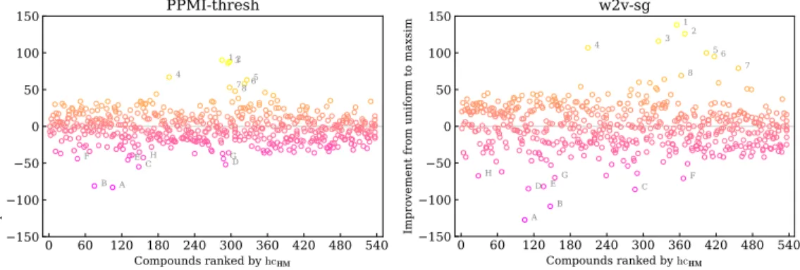
Nominal compounds such as red wine and nut case display a continuum of compositionality, with varying contributions from the components of the compound to its semantics. This article proposes a framework for compound compositionality prediction using distributional semantic models, evaluating to what extent they capture idiomaticity compared to human judgments. For evaluation, we introduce data sets containing human judgments in three languages: English, French, and Portuguese. The results obtained reveal a high agreement between the models and human predictions, suggesting that they are able to incorporate information about idiomaticity. We also present an in-depth evaluation of various factors that can affect prediction, such as model and corpus parameters and compositionality operations. General crosslingual analyses reveal the impact of morphological variation and corpus size in the ability of the model to predict compositionality, and of a uniform combination of the components for best results.
1. Introduction
It is a universally acknowledged assumption that the meaning of phrases, expressions, or sentences can be determined by the meanings of their parts and by the rules used
Submission received: 4 December 2017; revised version received: 22 June 2018; accepted for publication: 8 August 2018.
doi:10.1162/COLI a 00341
to combine them. Part of the appeal of this principle of compositionality1 is that it
implies that a meaning can be assigned even to a new sentence involving an unseen combination of familiar words (Goldberg 2015). Indeed, for natural language processing (NLP), this is an attractive way of linearly deriving the meaning of larger units from their components, performing the semantic interpretation of any text.
For representing the meaning of individual words and their combinations in com-putational systems, distributional semantic models (DSMs) have been widely used. DSMs are based on Harris’ distributional hypothesis that the meaning of a word can be inferred from the context in which it occurs (Harris 1954; Firth 1957). In DSMs, words are usually represented as vectors that, to some extent, capture cooccurrence patterns in corpora (Lin 1998; Landauer, Foltz, and Laham 1998; Mikolov et al. 2013; Baroni, Dinu, and Kruszewski 2014). Evaluation of DSMs has focused on obtaining accurate semantic representations for words, and state-of-the-art models are already capable of obtaining a high level of agreement with human judgments for predicting synonymy or similarity between words (Freitag et al. 2005; Camacho-Collados, Pilehvar, and Navigli 2015; Lapesa and Evert 2017) and for modeling syntactic and semantic analogies be-tween word pairs (Mikolov, Yih, and Zweig 2013). These representations for individual words can also be combined to create representations for larger units such as phrases, sentences, and even whole documents, using simple additive and multiplicative vector operations (Mitchell and Lapata 2010; Reddy, McCarthy, and Manandhar 2011; Mikolov et al. 2013; Salehi, Cook, and Baldwin 2015), syntax-based lexical functions (Socher et al. 2012), or matrix and tensor operations (Baroni and Lenci 2010; Bride, Van de Cruys, and Asher 2015). However, it is not clear to what extent this approach is adequate in the case of idiomatic multiword expressions (MWEs). MWEs fall into a wide spectrum of compositionality; that is, some MWEs are more compositional (e.g., olive oil) while others are more idiomatic (Sag et al. 2002; Baldwin and Kim 2010). In the latter case, the meaning of the MWE may not be straightforwardly related to the meanings of its parts, creating a challenge for the principle of compositionality (e.g., snake oil as a product of questionable benefit, not necessarily an oil and certainly not extracted from snakes).
In this article, we discuss approaches for automatically detecting to what extent the meaning of an MWE can be directly computed from the meanings of its compo-nent words, represented using DSMs. We evaluate how accurately DSMs can model the semantics of MWEs with various levels of compositionality compared to human judgments. Since MWEs encompass a large amount of related but distinct phenomena, we focus exclusively on a subcategory of MWEs: nominal compounds. They represent an ideal case study for this work, thanks to their relatively homogeneous syntax (as opposed to other categories of MWEs such as verbal idioms) and their pervasiveness in language. We assume that models able to predict the compositionality of nominal compounds could be generalized to other MWE categories by addressing their vari-ability in future work. Furthermore, to determine to what extent these approaches are also adequate cross-lingually, we evaluate them in three languages: English, French, and Portuguese.
Given that MWEs are frequent in languages (Sag et al. 2002), identifying idiomatic-ity and producing accurate semantic representations for compositional and idiomatic cases is of relevance to NLP tasks and applications that involve some form of semantic processing, including semantic parsing (Hwang et al. 2010; Jagfeld and van der Plas 2015), word sense disambiguation (Finlayson and Kulkarni 2011; Schneider et al. 2016),
and machine translation (Ren et al. 2009; Carpuat and Diab 2010; Cap et al. 2015; Salehi et al. 2015). Moreover, the evaluation of DSMs on tasks involving MWEs, such as compositionality prediction, has the potential to drive their development towards new directions.
The main hypothesis of our work is that, if the meaning of a compositional nominal compound can be derived from a combination of its parts, this translates in DSMs as similar vectors for a compositional nominal compound and for the combination of the vectors of its parts using some vector operation, that we refer to as composition
function. Conversely we can use the lack of similarity between the nominal compound vector representation and a combination of its parts to detect idiomaticity. Further-more, we hypothesize that accuracy in predicting compositionality depends both on the characteristics of the DSMs used to represent expressions and their components and on the composition function adopted. Therefore, we have built 684 DSMs and performed an extensive evaluation, involving over 9,072 analyses, investigating various types of DSMs, their configurations, the corpora used to train them, and the composition function used to build vectors for expressions.2
This article is structured as follows. Section 2 presents related work on distributional semantics, compositionality prediction, and nominal compounds. Section 3 presents the data sets created for our evaluation. Section 4 describes the compositionality prediction framework, along with the composition functions which we evaluate. Section 5 spec-ifies the experimental setup (corpora, DSMs, parameters, and evaluation measures). Section 6 presents the overall results of the evaluated models. Sections 7 and 8 evaluate the impact of DSM and corpus parameters, and of composition functions on composi-tionality prediction. Section 9 discusses system predictions through an error analysis. Section 10 summarizes our conclusions. Appendix A contains a glossary, Appendix B presents extra sanity-check experiments, Appendix C contains the questionnaire used for data collection, and Appendices D, E, and F list the compounds in the data sets.
2. Related Work
The literature on distributional semantics is extensive (Lin 1998; Turney and Pantel 2010; Baroni and Lenci 2010; Mohammad and Hirst 2012), so we provide only a brief introduc-tion here, underlining their most relevant characteristics to our framework (Secintroduc-tion 2.1). Then, we define compositionality prediction and discuss existing approaches, focusing on distributional techniques for multiword expressions (Section 2.2). Our framework is evaluated on nominal compounds, and we discuss their relevant properties (Section 2.3) along with existing data sets for evaluating compositionality prediction (Section 2.4).
2 This article significantly extends and updates previous publications:
1. We consolidate the description of the data sets introduced in Ramisch et al. (2016) and Ramisch, Cordeiro, and Villavicencio (2016) by adding details about data collection, filtering, and results of a thorough analysis studying the correlation between compositionality and related variables.
2. We extend the compositionality prediction framework described in Cordeiro, Ramisch, and
Villavicencio (2016) by adding and evaluating new composition functions and DSMs.
3. We extend the evaluation reported in Cordeiro et al. (2016) not only by adding Portuguese,
but also by evaluating additional parameters: corpus size, composition functions, and new DSMs.
2.1 Distributional Semantic Models
Distributional semantic models (DSMs) use context information to represent the mean-ing of lexical units as vectors. These vectors are built assummean-ing the distributional
hypothesis, whose central idea is that the meaning of a word can be learned based on the contexts where it appears—or, as popularized by Firth (1957), “you shall know a word by the company it keeps.”
Formally, a DSM attempts to encode the meaning of each target word wi of a
vocabulary V as a vector of real numbers v(wi) in R|V|. Each component of v(wi) is a
function of the co-occurrence between wi and the other words in the vocabulary (its
contexts wc). This function can be simply a co-occurrence count c(wi, wc), or some
mea-sure of the association between wiand each wc, such as pointwise mutual information
(PMI, Church and Hanks [1990], Lin [1999]) or positive PMI (PPMI, Baroni, Dinu, and Kruszewski [2014]; Levy, Goldberg, and Dagan [2015]).
In DSMs, co-occurrence can be defined as two words co-occurring in the same document, sentence, or sentence fragment in a corpus. Intrasentential models are often based on a sliding window; that is, a context word wcco-occurs within a certain window
of W words around the target wi. Alternatively, co-occurrence can also be based on
syntactic relations obtained from parsed corpora, where a context word wc appears
within specific syntactic relations with wi(Lin 1998; Pad ´o and Lapata 2007; Lapesa and
Evert 2017).
The set of all vectors v(wi),∀wi∈V can be represented as a sparse co-occurrence
matrix V×V→R. Given that most word pairs in this matrix co-occur rarely (if ever),
a threshold on the number of co-occurrences is often applied to discard irrelevant pairs. Additionally, co-occurrence vectors can be transformed to have a significantly smaller number of dimensions, converting vectors in R|V| into vectors in Rd, with d |V|.3 Two solutions are commonly employed in the literature. The first one consists in using context thresholds, where all target–context pairs that do not belong to the top-d most relevant pairs are discarded (Salehi, Cook, and Baldwin 2014; Padr ´o et al. 2014b). The second solution consists in applying a dimensionality reduction technique such as singular value decomposition on the co-occurrence matrix where only the d largest singular values are retained (Deerwester et al. 1990). Similar techniques focus on the factorization of the logarithm of the co-occurrence matrix (Pennington, Socher, and Manning 2014) and on alternative factorizations of the PPMI matrix (Salle, Villavicencio, and Idiart 2016).
Alternatively, DSMs can be constructed by training a neural network to predict target–context relationships. For instance, a network can be trained to predict a target word wi among all possible words in V given as input a window of surrounding
context words. This is known as the continuous bag-of-words model. Conversely, the network can try to predict context words for a target word given as input, and this is known as the skip-gram model (Mikolov et al. 2013). In both cases, the network training procedure allows encoding in the hidden layer semantic information about words as a side effect of trying to solve the prediction task. The weight parameters that connect the unity representing wi with the d-dimensional hidden layer are taken as its vector
representation v(wi).
There are a number of factors that may influence the ability of a DSM to accurately learn a semantic representation. These include characteristics of the training corpus such
as size (Mikolov, Yih, and Zweig 2013) as well as frequency thresholds and filters (Ferret 2013; Padr ´o et al. 2014b), genre (Lapesa and Evert 2014), preprocessing (Pad ´o and Lapata 2003, 2007), and type of context (window vs. syntactic dependencies) (Agirre et al. 2009; Lapesa and Evert 2017). Characteristics of the model include the choice of association and similarity measures (Curran and Moens 2002), dimensionality reduction strategies (Van de Cruys et al. 2012), and the use of subsampling and negative sampling techniques (Mikolov, Yih, and Zweig 2013). However, the particular impact of these factors on the quality of the resulting DSM may be heterogeneous and depends on the task and model (Lapesa and Evert 2014). Because there is no consensus about a single optimal model that works for all tasks, we compare a variety of models (Section 5) to determine which are best suited for our compositionality prediction framework.
2.2 Compositionality Prediction
Before adopting the principle of compositionality to determine the meaning of a larger unit, such as a phrase or multiword expression (MWE), it is important to determine whether it is idiomatic or not.4This problem, known as compositionality prediction, can be solved using methods that measure directly the extent to which an expression is constructed from a combination of its parts, or indirectly via language-dependent properties of MWEs linked to idiomaticity like the degree of determiner variability and morphological flexibility (Fazly, Cook, and Stevenson 2009; Tsvetkov and Wintner 2012; Salehi, Cook, and Baldwin 2015; K ¨oper and Schulte im Walde 2016). In this article, we focus on direct prediction methods in order to evaluate the target languages under sim-ilar conditions. Nonetheless, this does not exclude the future integration of information used by indirect prediction methods, as a complement to the methods discussed here.
For direct prediction methods, three ingredients are necessary. First, we need vector representations of single-word meanings, such as those built using DSMs (Section 2.1). Second, we need a mathematical model of how the compositional meaning of a phrase is calculated from the meanings of its parts. Third, we need the compositionality measure itself, which estimates the similarity between the compositionally constructed meaning of a phrase and its observed meaning, derived from corpora. There are a number of alternatives for each of the ingredients, and throughout this article we call a specific choice of the three ingredients a compositionality prediction configuration.
Regarding the second ingredient, that is, the mathematical model of compositional meaning, the most natural choice is the additive model (Mitchell and Lapata 2008). In the additive model, the compositional meaning of a phrase w1w2. . .wnis calculated as
a linear combination of the word vectors of its components:P
iβiv(wi), where v(wi) is a
d-dimensional vector for each word wi, and theβicoefficients assign different weights
to the representation of each word (Reddy, McCarthy, and Manandhar 2011; Schulte im Walde, M ¨uller, and Roller 2013; Salehi, Cook, and Baldwin 2015). These weights can capture the asymmetric contribution of each of the components to the semantics of the whole phrase (Bannard, Baldwin, and Lascarides 2003; Reddy, McCarthy, and Manandhar 2011). For example, in flea market, it is the head (market) that has a clear contribution to the overall meaning, whereas in couch potato it is the modifier (couch).
The additive model can be generalized to use a matrix of multiplicative coefficients, which can be estimated through linear regression (Guevara 2011). This model can be
4 The task of determining whether a phrase is compositional is closely related to MWE discovery (Constant et al. 2017), which aims to automatically extract MWE lists from corpora.
further modified to learn polynomial projections of higher degree, with quadratic pro-jections yielding particularly promising results (Yazdani, Farahmand, and Henderson 2015). These models come with the caveat of being supervised, requiring some amount of pre-annotated data in the target language. Because of these requirements, our study focuses on unsupervised compositionality prediction methods only, based exclusively on automatically POS-tagged and lemmatized monolingual corpora.
Alternatives to the additive model include the multiplicative model and its vari-ants (Mitchell and Lapata 2008). However, results suggest that this representation is inferior to the one obtained through the additive model (Reddy, McCarthy, and Manandhar 2011; Salehi, Cook, and Baldwin 2015). Recent work on predicting intra-compound semantics also supports that additive models tend to yield better results than multiplicative models (Hartung et al. 2017).
The third ingredient is the measure of similarity between the compositionally constructed vector and its actual corpus-based representation. Cosine similarity is the most commonly used measure for compositionality prediction in the literature (Schone and Jurafsky 2001; Reddy, McCarthy, and Manandhar 2011; Schulte im Walde, M ¨uller, and Roller 2013; Salehi, Cook, and Baldwin 2015). Alternatively, one can calculate the overlap between the distributional neighbors of the whole phrase and those of the component words (McCarthy, Keller, and Carroll 2003), or the number of single-word distributional neighbors of the whole phrase (Riedl and Biemann 2015).
2.3 Nominal Compounds
Instead of covering compositionality prediction for MWEs in general, we focus on a particular category of phenomena represented by nominal compounds. We define a
nominal compoundas a syntactically well-formed and conventionalized noun phrase containing two or more content words, whose head is a noun.5 They are
convention-alized (or institutionconvention-alized) in the sense that their particular realization is statistically idiosyncratic, and their constituents cannot be replaced by synonyms (Sag et al. 2002; Baldwin and Kim 2010; Farahmand, Smith, and Nivre 2015). Their semantic interpre-tation may be straightforwardly compositional, with contributions from both elements (e.g., climate change), partly compositional, with contribution mainly from one of the elements (e.g., grandfather clock), or idiomatic (e.g., cloud nine) (Nakov 2013).
The syntactic realization of nominal compounds varies across languages. In English, they are often expressed as a sequence of two nouns, with the second noun as the syntactic head, modified by the first noun. This is the most frequently annotated POS-tag pattern in the MWE-annotated DiMSUM English corpus (Schneider et al. 2016). In French and Portuguese, they often assume the form of adjective–noun or noun– adjective pairs, where the adjective modifies the noun. Examples of such constructions include the adjective–noun compound FR petite annonce (lit. small announcement ‘classi-fied ad’) and the noun–adjective compound PT buraco negro (lit. hole black ‘black hole’).6
Additionally, compounds may also involve prepositions linking the modifier with the head, as in the case of FR cochon d’Inde (lit. pig of India ‘guinea pig’) and PT dente de leite (lit. tooth of milk ‘milk tooth’). Because prepositions are highly polysemous and their representation in DSMs is tricky, we do not include compounds containing prepositions
5 The terms noun compound and compound noun are usually reserved for nominal compounds formed by sequences of nouns only, typical of Germanic languages but not frequent in Romance languages. 6 In this article, examples are preceded by their language codes: EN for English, FR for French, and PT for
in this article. Hence, we focus on 2-word nominal compounds of the form noun1–noun2
(in English), and noun–adjective and adjective–noun (in the three languages).
Regarding the meaning of nominal compounds, the implicit relation between the components of compositional compounds can be described in terms of free paraphrases involving verbs, such as flu virus as virus that causes/creates flu (Nakov 2008),7or prepo-sitions, such as olive oil as oil from olives (Lauer 1995). These implicit relations can often be seen explicitly in the equivalent expressions in other languages (e.g., FR huile d’olive and PT azeite de oliva for EN olive oil).
Alternatively, the meaning of compositional nominal compounds can be described using a closed inventory of relations which make the role of the modifier explicit with respect to the head noun, including syntactic tags such as subject and object, and seman-tic tags such as instrument and location (Girju et al. 2005). The degree of compositionality of a nominal compound can also be represented using numerical scores (Section 2.4) to indicate to what extent the component words allow predicting the meaning of the whole (Reddy, McCarthy, and Manandhar 2011; Roller, Schulte im Walde, and Scheible 2013; Salehi et al. 2015). The latter is the representation that we adopted in this article.
2.4 Numerical Compositionality Data sets
The evaluation of compositionality prediction models can be performed extrinsically or intrinsically. In extrinsic evaluation, compositionality information can be used to decide how a compound should be treated in NLP systems such as machine translation or text simplification. For instance, for machine translation, idiomatic compounds need to be treated as atomic phrases, as current methods of morphological compound processing cannot be applied to them (Stymne, Cancedda, and Ahrenberg 2013; Cap et al. 2015).
Although potentially interesting, extrinsic evaluation is not straightforward, as results may be influenced both by the compositionality prediction model and by the strategy for integration of compositionality information into the NLP system. Therefore, most related work focuses on an intrinsic evaluation, where the compositionality scores produced by a model are compared to a gold standard, usually a data set where nominal compound semantics have been annotated manually. Intrinsic evaluation thus requires the existence of data sets where each nominal compound has one (or several) numerical scores associated with it, indicating its compositionality. Annotations can be provided by expert linguist annotators or by crowdsourcing, often requiring that several annotators judge the same compound to reduce the impact of subjectivity on the scores. Relevant compositionality data sets of this type are listed below, some of which were used in our experiments.
• Reddy, McCarthy, and Manandhar (2011) collected judgments for a set of 90 English noun–noun (e.g., zebra crossing) and adjective–noun (e.g., sacred cow) compounds, in terms of three numerical scores: the compositionality of the compound as a whole and the literal contribution of each of its parts individually, using a scale from 0 to 5. The data set was built through crowdsourcing, and the final scores are the average of 30 judgments per compound.This data set will be referred to as Reddy in our experiments.
7 Nakov (2008) also proposes a method for automatically extracting paraphrases from the web to classify nominal compounds. This was extended in a SemEval 2013 task, where participants had to rank free paraphrases according to the semantic relations in the compounds (Hendrickx et al. 2013).
• Farahmand, Smith, and Nivre (2015) collected judgments for 1,042 English noun–noun compounds. Each compound has binary judgments regarding non-compositionality and conventionalization given by four expert annotators (both native and non-native speakers). A hard threshold is applied so that compounds are considered as noncompositional if at least two annotators say so (Yazdani, Farahmand, and Henderson 2015), and the total compositionality score is given by the sum of the four binary judgments. This data set will be referred to as Farahmand in our experiments.
• Kruszewski and Baroni (2014) built the Norwegian Blue Parrot data set, containing judgments for modifier-head phrases in English. The judgments consider whether the phrase is (1) an instance of the concept denoted by the head (e.g., dead parrot and parrot) and (2) a member of the more general concept that includes the head (e.g., dead parrot and pet), along with typicality ratings, with 5,849 judgments in total.
• Roller, Schulte im Walde, and Scheible (2013) collected judgments for a set of 244 German noun–noun compounds, each compound with an average of around 30 judgments on a compositionality scale from 1 to 7, obtained through crowdsourcing. The resource was later enriched with feature norms (Roller and Schulte im Walde 2014).
• Schulte im Walde et al. (2016) collected judgments for a set of 868 German noun–noun compounds, including human judgments of compositionality on a scale of 1 to 6. Compounds are judged by multiple annotators, and the final compositionality score is the average across annotators. The data set is also annotated for in-corpus frequency, productivity, and ambiguity, and a subset of 180 compounds has been selected for balancing these variables. The annotations were performed by the authors, linguists, and through crowdsourcing. For the balanced subset of 180 compounds, compositionality annotations were performed by experts only, excluding the authors.
For a multilingual evaluation, in this work, we construct two data sets, one for French and one for Portuguese compounds, and extend the Reddy data set for English using the same protocol as Reddy, McCarthy, and Manandhar (2011).
3. Creation of a Multilingual Compositionality Data set
In Section 3.1, we describe the construction of data sets of 180 compounds for French (FR-comp) and Portuguese (PT-comp). For English, the complete data set contains 280 compounds, of which 190 are new and 90 come from the Reddy data set. We use 180 of these (EN-comp) for cross-lingual comparisons (90 from the original Reddy data set combined with 90 new ones from EN-comp90), and 100 new compounds as held-out data
(EN-compExt), to evaluate the robustness of the results obtained (Section 6.3). These data
sets containing compositionality scores for 2–word nominal compounds are used to evaluate our framework (Section 4), and we discuss their characteristics in Section 3.2.8
8 For English, only EN-comp90and EN-compExt(90 and 100 new compounds, respectively) are considered.
3.1 Data Collection
For each of the target languages, we collected, via crowdsourcing, a set of numerical scores corresponding to the level of compositionality of the target nominal compounds. We asked non-expert participants to judge each compound considering three sentences where the compound occurred. After reading the sentences, participants assess the degree to which the meaning of the compound is related to the meanings of its parts. This follows from the assumption that a fully compositional compound will have an interpretation whose meaning stems from both words (e.g., lime tree as a tree of limes), while a fully idiomatic compound will have a meaning that is unrelated to its compo-nents (e.g., nut case as an eccentric person).
Our work follows the protocol proposed by Reddy, McCarthy, and Manandhar (2011), where compositionality is explained in terms of the literality of the individual parts. This type of indirect annotation does not require expert linguistic knowledge, and still provides reliable data, as we show later. For each language, data collection involved four steps: compound selection, sentence selection, questionnaire design, and data aggregation.
Compound Selection. For each data set, we manually selected nominal compounds from dictionaries, corpus searches, and by linguistic introspection, maintaining an equal pro-portion of compounds that are compositional, partly compositional, and idiomatic.9We considered them to be compositional if their semantics are related to both components (e.g., benign tumor), partly compositional if their semantics are related to only one of the components (e.g., grandfather clock), and idiomatic if they are not directly related to either (e.g., old flame). This preclassification was used only to select a balanced set of compounds and was not shown to the participants nor used at any later stage. For all languages, all compounds are required to have a head that is unambiguously a noun, and additionally for French and Portuguese, all compounds have an adjective as modifier.
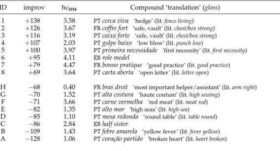
Sentence Selection. Compounds may be polysemous (e.g., FR bras droit may mean most reliable helper or literally right arm). To avoid any potential sense uncertainty, each compound was presented to the participants with the same sense in three sentences. These sentences were manually selected from the WaC corpora: ukWaC (Baroni et al. 2009), frWaC, and brWaC (Boos, Prestes, and Villavicencio 2014), presented in detail in Section 5.
Questionnaire Design. For each compound, after reading three sentences, participants are asked to:
• provide synonyms for the compound in these sentences. The synonyms are used as additional validation of the quality of the judgments: if unrelated words are provided, the answers are discarded.
• assess the contribution of the head noun to the meaning of the compound (e.g., is a busy bee always literally a bee?)
9 We have not attempted to select compounds that are translations of each other, as a compound in a given language may be realized differently in the other languages.
• assess the contribution of the modifier noun or adjective to the meaning of the compound (e.g., is a busy bee always literally busy?)
• assess the degree to which the compound can be seen as a combination of its parts (e.g., is a busy bee always literally a bee that is busy?)
Participants answer the last three items using a Likert scale from 0 (idiomatic/non-literal) to 5 (compositional/(idiomatic/non-literal), following Reddy, McCarthy, and Manandhar (2011). To qualify for the task, participants had to submit demographic information confirming that they are native speakers, and to undergo training in the form of four example questions with annotated answers in an external form (see Appendix C for details). Data Aggregation. For English and French, we collected answers using Amazon Mechan-ical Turk (AMT), manually removing answers that were not from native speakers or where the synonyms provided were unrelated to the target compound sense. Because AMT has few Brazilian Portuguese native speakers, we developed an in-house web inter-face for the questionnaire, which was sent out to Portuguese-speaking NLP mailing lists.
For a given compound and question we calculate aggregated scores as the arith-metic averages of all answers across participants. We will refer to these averaged scores as the human compositionality score (hc)s. We average the answers to the three questions independently, generating three scores: hcHfor the head noun, hcM for the modifier, and hcHMfor the whole compound. In our framework, we try to predict hcHM automatically (Section 5). To assess the variability of the answers (Section 3.2.1), we also calculate the standard deviation across participants for each question (σH,σM, andσHM).
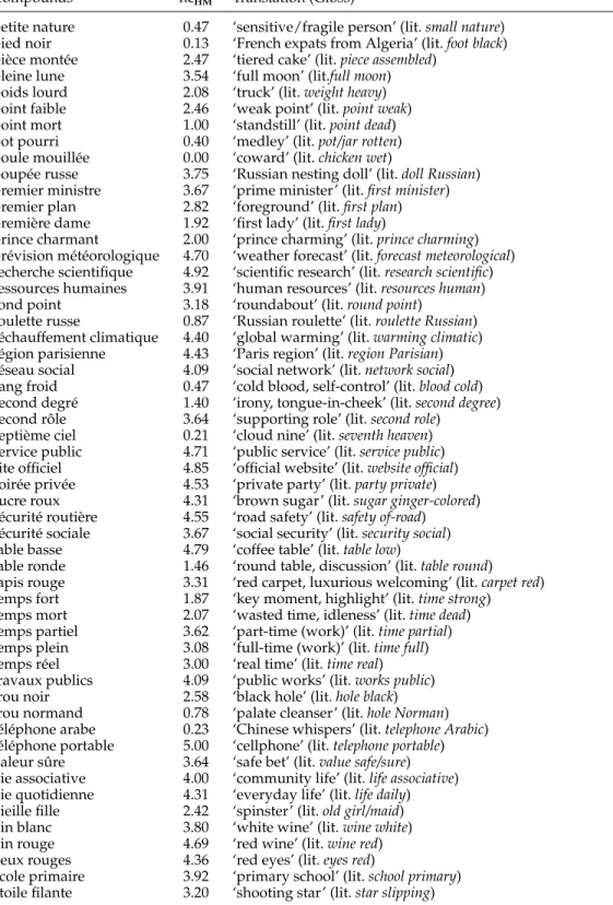
The list of compounds, their translations, glosses, and compositionality scores are given in Appendices D (EN-comp90and EN-compExt), E (FR-comp), and F (PT-comp).10
3.2 Data set Analysis
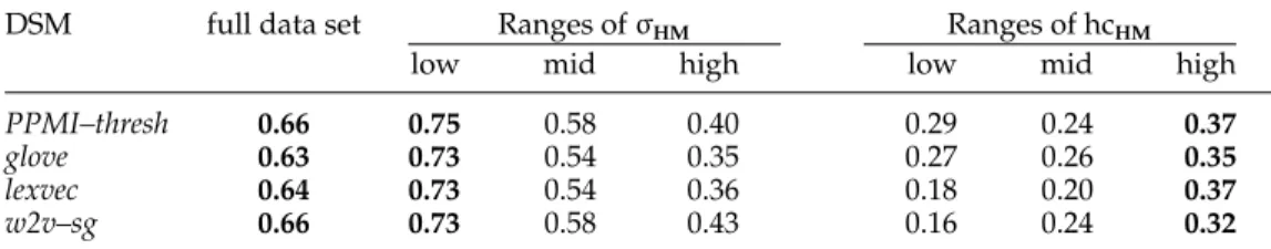
In this section, we present different measures of agreement among participants (Sec-tion 3.2.1) and examine possible correla(Sec-tions between composi(Sec-tionality scores, familiar-ity, and conventionalization (Section 3.2.2) in the data sets created for this article. 3.2.1 Measuring Data set Quality. To assess the quality of the collected human composi-tionality scores, we use standard deviation and inter-annotator agreement scores. Standard Deviation (σand Pσ>1.5) . The standard deviation (σ) of the participants’
an-swers can be used as an indication of their agreement: for each compound and for each of the three questions, small σ values suggest greater agreement. In addition, if the instructions are clear,σ can also be seen as an indication of the level of difficulty of the task. In other words, all other things being equal, compounds with larger σ can be considered intrinsically harder to analyze by the participants. For each data set, we consider two aggregated metrics based onσ:
• σ— The average ofσin the data set.
• Pσ>1.5— The proportion of compounds whoseσis higher than 1.5.
Table 1
Average number of answers per compound n, average standard deviation σ, proportion of high standard deviation Pσ>1.5, for the compound (HM), head (H), and modifier (M).
Data set n σHM σH σM PσHM>1.5 PσH>1.5 PσM>1.5 FR-comp 14.9 1.15 1.08 1.21 22.78% 24.44% 30.56% PT-comp 31.8 1.22 1.09 1.20 14.44% 17.22% 19.44% EN-comp90 18.8 1.17 1.05 1.18 18.89% 16.67% 27.78% EN-compExt 22.6 1.21 1.27 1.16 17.00% 29.00% 18.00% Reddy 28.4 0.99 0.94 0.89 5.56% 11.11% 8.89%
Table 1 presents the result of these metrics when applied to our in-house data sets, as well as to the original Reddy data set. The column n indicates the average number of answers per compound, while the other six columns present the values ofσand Pσ>1.5
for compound (HM), head-only (H), and modifier-only (M) scores.
These values are below what would be expected for random decisions (σrand '
1.71, for the Likert scale). Although our data sets exhibit higher variability than Reddy, this may be partly due to the application of filters done by Reddy, McCarthy, and Manandhar (2011) to remove outliers.11 These values could also be due to the
collec-tion of fewer answers per compound for some of the data sets. However, there is no clear tendency in the variation of the standard deviation of the answers and the num-ber of participants n. The values ofσ are quite homogeneous, ranging from 1.05 for EN-comp90(head) to 1.27 for EN-compExt(head). The low agreement for modifiers may be
related to a greater variability in semantic relations between modifiers and compounds: these include material (e.g., brass ring), attribute (e.g., black cherry), and time (e.g., night owl).
Figure 1(a) shows standard deviation (σHM, σH, and σM) for each compound of FR-comp as a function of its average compound score hcHM.12 For all three languages, greater agreement was found for compounds at the extremes of the compositionality scale (fully compositional or fully idiomatic) for all scores. These findings can be partly explained by end-of-scale effects, that result in greater variability for the intermedi-ate scores in the Likert scale (from 1 to 4) that correspond to the partly composi-tional cases. Hence, we expect that it will be easier to predict the composicomposi-tionality of idiomatic/compositional compounds than of partly compositional ones.
Inter-Annotator Agreement (α). To measure inter-annotator agreement of multiple partici-pants, taking into account the distance between the ordinal ratings of the Likert scale, we adopt theαscore (Artstein and Poesio 2008). Theαscore is more appropriate for ordinal data than traditional agreement scores for categorical data, such as Cohen’s and Fleiss’
κ (Cohen 1960; Fleiss and Cohen 1973). However, due to the use of crowdsourcing, most participants rated only a small number of compounds with very limited chance of overlap among them: the average number of answers per participant is 13.6 for EN-comp90, 10.2 for EN-compExt, 33.7 for FR-comp, and 53.5 for PT-comp. Because the
11 Participants with negative correlation with the mean, and answers farther than±1.5 from the mean. 12 Only FR-comp is shown as the other data sets display similar patterns.
0 20 40 60 80 100 120 140 160 180 Compounds ranked by hcHM 0.0 0.5 1.0 1.5 2.0 St an da rd d ev iat io n ( σ )
(a) Standard deviation (FR-comp)
σH (head only) σM (modifier only) σHM (compound) 0 20 40 60 80 100 120 140 160 180 Compounds ranked by hcHM 0 1 2 3 4 5 Compositionality score (hc)
(b) Compositionality (FR-comp)
hcH (head only) hcM (modifier only) hcHM (compound) Figure 1Left: Standard deviations (σH, σM, and σHM) as a function of hcHMin FR-comp. Right: Average
compositionality (hcH, hcM, and hcHM) as a function of hcHMin FR-comp.
α score assumes that each participant rates all the items, we focus on the answers provided by three of the participants, who rated the whole set of 180 compounds in PT-comp.
Using a linear distance schema between the answers,13we obtain an agreement of
α= .58 for head-only,α= .44 for modifier-only, andα= .44 for the whole compound. To further assess the difficulty of this task, we also calculate α for a single expert annotator, judging the same set of compounds after an interval of one month. The scores wereα= .69 for the head andα= .59 for both the compound and for the modifier. The Spearman correlation between these two annotations performed by the same expert is ρ=0.77 for hcHM. This can be seen as a qualitative upper bound for automatic compositionality prediction on PT-comp.
3.2.2 Compositionality, Familiarity, and Conventionalization. Figure 1(b) shows the average scores (hcHM, hcH, and hcM) for the compounds ranked according to the average com-pound score hcHM. Although this figure is for FR-comp, similar patterns were found for the other data sets. For all three languages, the human compositionality scores provide additional confirmation that the data sets are balanced, with the compound scores (hcHM) being distributed linearly along the scale. Furthermore, we have calculated the average hcHMvalues separately for the compounds in each of the three compositionality classes used for compound selection: idiomatic, partly compositional and compositional (Section 3.1). These averages are, respectively, 1.0, 2.4, and 4.0 for EN-comp90; 1.1, 2.4,
and 4.2 for EN-compExt; 1.3, 2.7, and 4.3 for FR-comp; and 1.3, 2.5, and 3.9 for PT-comp,
indicating that our attempt to select a balanced number of compounds from each class is visible in the collected hcHMscores.
Additionally, the human scores also suggest an asymmetric impact of the non-literal parts over the compound: whenever participants judged an element of the compound as non-literal, the whole compound was also rated as idiomatic. Thus, most head and modifier scores (hcH and hcM) are close to or above the diagonal line in Figure 1(b). In other words, a component of the compound is seldom rated as less literal than the compositionality of the whole compound hcHM, although the opposite is more common.
0 1 2 3 4 5 hcHM 0 1 2 3 4 5 hcH ⊗ hcM ⊗= arithmetic mean ⊗= geometric mean
Linear regr. of arith. mean Linear regr. of geom. mean
Figure 2
Relation between hcH⊗ hcMand hcHMin FR-comp, using arithmetic and geometric means.
Table 2
Spearman ρ correlation between compositionality, frequency, and PMI for the three data sets.
Data set frequency PMI
FR-comp 0.598 (p < 10−18) 0.164 (p > 0.01) PT-comp 0.109 (p > 0.1) 0.076 (p > 0.1) EN-comp90 0.305 (p < 10−2) −0.024 (p > 0.1) EN-compExt 0.384 (p < 10−5) 0.138 (p > 0.1)
To evaluate if it is possible to predict hcHMfrom the hcHand hcM, we calculate the arithmetic and geometric means between hcH and hcM for each compound. Figure 2 shows the linear regression of both measures for FR-comp. The goodness of fit is r2
arith= .93 for the arithmetic mean, and r2geom= .96 for the geometric mean, confirming
that they are good predictors of hcHM.14 Thus, we assume that hcHMsummarizes hcH and hcM, and focus on predicting hcHMinstead of hcHand hcMseparately. These find-ings also inspired the pcarithand pcgeomcompositionality prediction functions (Section 4). To examine whether there is an effect of the familiarity of a compound on hc scores, in particular if more idiomatic compounds need to be more familiar, we also calculated the correlation between the compositionality score for a compound hcHM and its frequency in a corpus, as a proxy for familiarity. In this case we used the WaC corpora and calculated the frequencies based on the lemmas. The results, in Table 2, show a statistically significant positive Spearman correlation ofρ=0.305 for EN-comp90,
ρ=0.384 for EN-compExt, and ρ=0.598 for FR-comp, indicating that, contrary to our
expectations, compounds that are more frequent tend to be assigned higher composi-tionality scores. However, frequency alone is not enough to predict composicomposi-tionality, and further investigation is needed to determine if compositionality and frequency are also correlated with other factors.
We also analyzed the correlation between compositionality and conventionaliza-tion to determine if more idiomatic compounds correspond to more convenconventionaliza-tionalized ones. We use PMI (Church and Hanks 1990) as a measure of conventionalization, as it indicates the strength of association between the components (Farahmand, Smith, and Nivre 2015). We found no statistically significant correlation between compositionality and PMI.
4. Compositionality Prediction Framework
We propose a compositionality prediction framework15 including the following
ele-ments: a DSM, created from corpora using existing state-of-the-art models that gen-erate corpus-derived vectors16 for compounds w
1w2and for their components w1 and
w2; a composition function; and a set of predicted compositionality scores (pc). The
framework, shown in Figure 3, is evaluated by measuring the correlation between the scores predicted by the models (pc) and the human compositionality scores (hc) for the list of compounds in our data sets (Section 3). The predicted compositionality scores are obtained from the cosine similarity between the corpus-derived vector of the compound, v(w1w2), and the compositionally constructed vector, vβ(w1, w2):
pcβ(w1w2)=cos( v(w1w2), vβ(w1, w2) ).
For vβ(w1, w2), we use the additive model (Mitchell and Lapata 2008), in which the
composition function is a weighted linear combination:
vβ(w1w2)= β||vv(w(whead)
head)||
+(1− β) v(wmod)
||v(wmod)||,
where whead(or wmod) indicates the head (or modifier) of the compound w1w2,|| · ||is the
Euclidean norm, andβ∈[0, 1] is a parameter that controls the relative importance of the head to the compound’s compositionally constructed vector. The normalization of both vectors allows taking only their directions into account, regardless of their norms, which are usually proportional to their frequency and irrelevant to meaning.
We define six compositionality scores based on pcβ. Three of them pchead(w1w2),
pcmod(w1w2), and pcuniform(w1w2), correspond to different assumptions about how we
model compositionality: if dependent on the head (β=1, for e.g., crocodile tears), on the modifier (β=0, for e.g., busy bee), or in equal measure on the head and modifier (β=1/2, for e.g., graduate student). The fourth score is based on the assumption that compositionality may be distributed differently between head and modifier for different compounds. We implement this idea by setting individually for each compound the
15 Implemented as feat compositionality.py in the mwetoolkit: http://mwetoolkit.sf.net. 16 Except when explicitly indicated, the term vector refers to corpus-derived vectors output by DSMs.
questionnairesquestionnaires w1 w2 compound vocabulary (list of compounds) DSM configuration DSM parameters processed corpus v(w1w2) v(w2) v(w1) corpusderived vectors vβ(w1,w2) compositionally constructed vectors composition function questionnaires Spearman ρ human comp. scores (hc) similarity function DSM predicted comp. scores (pc) + ≅ Figure 3
Schema of a compositionality prediction configuration based on a composition function. Thick arrows indicate corpus-based vectors of two-word compounds treated as a single token. The schema also covers the evaluation of the compositionality prediction configuration (top right).
value for β that yields maximal similarity in the predicted compositionality score, that is:17
pcmaxsim(w1w2)= max
0≤β≤1 pcβ(w1w2)
Two other scores are not based on the additive model and do not require a compo-sition function. Instead, they are based on the intuitive notion that compocompo-sitionality is related to the average similarity between the compound and its components:
pcavg(w1w2)=avg(pchead(w1w2), pcmod(w1w2))
We test two possibilities: the arithmetic mean pcarith(w1w2) considers that
composition-ality is linearly related to the similarity of each component of the compound, whereas the geometric mean pcgeom(w1w2) reflects the tendency found in human annotations to
assign compound scores hcHMcloser to the lowest score between that for the head hcH and for the modifier hcM(Section 3.2).
5. Experimental Setup
This section describes the common setup used for evaluating compositionality pre-diction, such as corpora (Section 5.1), DSMs (Section 5.2), and evaluation metrics (Section 5.3).
17 In practice, for the special case of two words, we do not need to perform parameter search forβ, which has a closed form obtained by solving the equation ∂
∂βpcβ(w1w2) = 0:
β= cos(w1w2,w1) − cos(w1w2,w2) × cos(w1,w2)
5.1 Corpora
In this work we used the lemmatized and POS-tagged versions of the WaC corpora not only for building DSMs, but also as sources of information about the target compounds for the analyses performed (e.g., in Sections 3.2.2, 9.1, and 9.2):
• for English, the ukWaC (Baroni et al. 2009), with 2.25 billion tokens, parsed with MaltParser (Nivre, Hall, and Nilsson 2006);
• for French, the frWaC with 1.61 billion tokens preprocessed with TreeTagger (Schmid 1995); and
• for Brazilian Portuguese, a combination of brWaC (Boos, Prestes, and Villavicencio 2014), Corpus Brasileiro,18and all Wikipedia entries,19with a
total of 1.91 billion tokens, all parsed with PALAVRAS (Bick 2000).
For all compounds contained in our data sets, we transformed their occur-rences into single tokens by joining their component words with an underscore (e.g., EN monkey business → monkey business and FR belle-m`ere → belle m`ere).20,21 To
han-dle POS-tagging and lemmatization irregularities, we retagged the compounds’ com-ponents using the gold POS and lemma in our data sets (e.g., for EN sitting duck, sit/verb duck/noun→sitting/adjective duck/noun). We also simplified all POS tags using coarse-grained labels (e.g., verb instead of vvz). All forms are then lowercased (surface forms, lemmas, and POS tags); and noisy tokens, with special characters, numbers, or punctuation, are removed. Additionally, ligatures are normalized for French (e.g., œ→
oe) and a spellchecker22 is applied to normalize words across English spelling variants
(e.g., color→colour).
To evaluate the influence of preprocessing on compositionality prediction (Sec-tion 7.3), we generated four versions of each corpus, with different levels of linguistic information. We expect lemmatization to reduce data sparseness by merging morpho-logically inflected variants of the same lemma:
1. surface+: the original raw corpus with no preprocessing, containing surface forms.
2. surface: stopword removal, generating a corpus of surface forms of content words.
3. lemmaPoS: stopword removal, lemmatization,23and POS-tagging;
generating a corpus of content words distinguished by POS tags, represented as lemma/POS-tag.
4. lemma: stopword removal and lemmatization; generating a corpus containing only lemmas of content words.
18 http://corpusbrasileiro.pucsp.br/cb/Inicial.html 19 Wikipedia articles downloaded on June 2016.
20 Hyphenated compounds are also re-tokenized with an underscore separator.
21 Therefore, in Section 5.2, the terms target/context words may actually refer to compounds. 22 https://hunspell.github.io
5.2 DSMs
In this section, we describe the state-of-the-art DSMs used for compositionality prediction.
Positive Pointwise Mutual Information (PPMI). In the models based on the PPMI matrix, the representation of a target word is a vector containing the PPMI association scores between the target and its contexts (Bullinaria and Levy 2012). The contexts are nouns and verbs, selected in a symmetric sliding window of W words to the left/right and weighted linearly according to their distance D to the target (Levy, Goldberg, and Dagan 2015).24We consider three models that differ in how the contexts are selected:
• In PPMI–thresh, the vectors are|V|-dimensional but only the top d contexts with highest PPMI scores for each target word are kept, while the others are set to zero (Padr ´o et al. 2014a).25
• In PPMI–TopK, the vectors are d-dimensional, and each of the d dimensions corresponds to a context word taken from a fixed list of k contexts, identical for all target words. We chose k as the 1, 000 most frequent words in the corpus after removing the top 50 most frequent words (Salehi, Cook, and Baldwin 2015).
• In PPMI–SVD, singular value decomposition is used to factorize the PPMI matrix and reduce its dimensionality from|V|to d.26We set the value of the context distribution smoothing factor to 0.75, and the negative
sampling factor to 5 (Levy, Goldberg, and Dagan 2015). We use the default minimum word count threshold of 5.
Word2vec (w2v). Word2vec27 relies on a neural network to predict target/context pairs (Mikolov et al. 2013). We use its two variants: continuous bag-of-words (w2v–cbow) and skip-gram (w2v–sg). We adopt the default configurations recommended in the documentation, except for: no hierarchical softmax, 25 negative samples, frequent-word down-sampling rate of 10−6, execution of 15 training iterations, and minimum word
count threshold of 5.
Global Vectors (glove). GloVe28 implements a factorization of the logarithm of the
posi-tional co-occurrence count matrix (Pennington, Socher, and Manning 2014). We adopt the default configurations from the documentation, except for: internal cutoff parameter xmax=75 and processing of the corpus in 15 iterations. For the corpora versions lemma
and lemmaPoS(Section 5.1), we use the minimum word count threshold of 5. For surface
and surface+, due to the larger vocabulary sizes, we use thresholds of 15 and 20.29
24 In previous work adjectives and adverbs were also included as contexts, but the results obtained with only verbs and nouns were better (Padr ´o et al. 2014a).
25 Vectors still have|V|dimensions but we use d as a shortcut to represent the fact that we only retain the most relevant target-context pairs for each target word.
26 https://bitbucket.org/omerlevy/hyperwords 27 https://code.google.com/archive/p/word2vec/ 28 https://nlp.stanford.edu/projects/glove/
Table 3
Summary of DSMs, their parameters, and evaluated parameter values. The combination of these DSMs and their parameter values leads to 228 DSM configurations evaluated per language (1 × 1 × 4 × 3 = 12 for PPMI–TopK, plus 6 × 3 × 4 × 3 = 216 for the other models).
DSM DIMENSION WORDFORM WINDOWSIZE
PPMI–TopK d = 1000 surface+, surface, lemma, lemmaPoS W = 1+1, W = 4+4, W = 8+8 PPMI–thresh d = 250, d = 500, d = 750 PPMI–SVD w2v–cbow w2v–sg glove lexvec
Lexical Vectors (lexvec). The LexVec model30 factorizes the PPMI matrix in a way that
penalizes errors on frequent words (Salle, Villavicencio, and Idiart 2016). We adopt the default configurations in the documentation, except for: 25 negative samples, sub-sampling rate of 10−6, and processing of the corpus in 15 iterations. Due to the
vocab-ulary sizes, we use a word count threshold of 10 for lemma and lemmaPoS, and 100 for
surface and surface+.31
5.2.1 DSM Parameters. In addition to model-specific parameters, the DSMs described above have some shared DSM parameters. We construct multiple DSM configurations by varying the values of these parameters. These combinations produce a total of 228 DSMs per language (see Table 3). In particular, we evaluate the influence of the following parameters on compositionality prediction:
• WINDOWSIZE: Number of context words to the left/right of the target
word when searching for target-context co-occurrence pairs. The assumption is that larger windows are better for capturing semantic relations (Jurafsky and Martin 2009) and may be more suitable for
compositionality prediction. We use window sizes of 1+1, 4+4, and 8+8.32
• DIMENSION: Number of dimensions of each vector. The underlying
hypothesis is that, the higher the number of dimensions, the more accurate the representation of the context is going to be. We evaluate our
framework with vectors of 250, 500, and 750 dimensions.
• WORDFORM: One of the four word-form and stopword removal variants used to represent a corpus, in Section 5.1: surface+, surface, lemma, and lemmaPoS. They represent different levels of specificity in the informational
content of the tokens, and may have a language-dependent impact on the performance of compositionality prediction.
30 https://github.com/alexandres/lexvec
31 This is in line with the authors’ threshold suggestions (Salle, Villavicencio, and Idiart 2016). 32 Common window sizes are between 1+1 and 10+10, but a few works adopt larger sizes like 16+16 or
5.3 Evaluation Metrics
To evaluate a compositionality prediction configuration, we calculate Spearman’s ρ
rank correlation between the predicted compositionality scores (pc)s and the human compositionality scores (hc)s for the compounds that appear in the evaluation data set. We mostly use the rank correlation instead of linear correlation (Pearson) because we are interested in the framework’s ability to order compounds from least to most compositional, regardless of the actual predicted values.
For English, besides the evaluation data sets presented in Section 3, we also use Reddy and Farahmand (see Section 2.4) to enable comparison with related work. For Farahmand, since it contains binary judgments33 instead of graded compositionality
scores, results are reported using the best F1(BF1) score, which is the highest F1score
found using the top n compounds classified as noncompositional, when n is varied (Yazdani, Farahmand, and Henderson 2015). For Reddy, we sometimes present Pearson scores to enable comparison with related work.
Because of the large number of compositionality prediction configurations eval-uated, we only report the best performance for each configuration over all possible DSM parameter values. The generalization of these analyses is then ensured using cross-validation and held-out data. To determine whether the difference between two prediction results are statistically different, we use nonparametric Wilcoxon’s sign-rank test.
6. Overall Results
In this section, we present the overall results obtained on the Reddy, Farahmand, EN-comp, FR-EN-comp, and PT-comp data sets, comparing all possible configurations (Sec-tion 6.1). To determine their robustness we also report evalua(Sec-tion for all languages using cross-validation (Section 6.2) and for English using the held-out data set EN-compExt(Section 6.3). All results reported in this section use the pcuniformfunction.
6.1 Distributional Semantic Models
Table 4 shows the highest overall values obtained for each DSM (columns) on each data set (rows). For English (Reddy, EN-comp, and Farahmand), the highest results for the compounds found in the corpus were obtained with w2v and PPMI–thresh, shown as the first value in each pair in Table 4. Not all compounds in the English data sets are present in our corpus. Therefore, we also report results adopting a fallback strategy (the second value). Because its impact depends on the data set, and the relative performance of the models is similar with or without it, for the remainder of the article we discuss only the results without fallback.34
The best w2v–cbow and w2v–sg configurations are not significantly different from each other, but both are different from PPMI–thresh (p<0.05). In a direct comparison
33 A compound is considered as noncompositional if at least 2 out of 4 annotators annotate it as noncompositional.
34 This refers to 5 out of 180 in EN-comp and 129 out of 1,042 in Farahmand. For these, the fallback strategy assigns the average compositionality score (Salehi, Cook, and Baldwin 2015). Although fallback produces slightly better results for EN-comp, it does the opposite for Farahmand, which contains a larger proportion of missing compounds (2.8% vs. 12.4%).
Table 4
Highest results for each DSM, using BF1for Farahmand data set, Pearson r for Reddy (r), and Spearman ρ for all the other data sets. For English, in each pair of values, the first is for the compounds found in the corpus, and the second uses fallback for missing compounds.
Data set PPMI–SVD PPMI–TopK PPMI–thresh glove lexvec w2v–cbow w2v–sg
Farahmand .487/.424 .435/.376 .472/.404 .400/.358 .449/.431 .512/.471 .507/.468 Reddy (r) .738/.726 .732/.717 .762/.768 .783/.787 .787/.787 .803/.798 .814/.814 Reddy (ρ) .743/.743 .706/.716 .791/.803 .754/.759 .774/.773 .796/.796 .812/.812 EN-comp .655/.666 .624/.632 .688/.704 .638/.651 .646/.658 .716/.730 .726/.741 FR-comp .584 .550 .702 .680 .677 .652 .653 PT-comp .530 .519 .602 .555 .570 .588 .586
with related work, our best result for the Reddy data set (Spearman ρ= .812, Pearson r= .814) improves upon the best correlation reported by Reddy, McCarthy, and Manandhar (2011) (ρ= .714), and by Salehi, Cook, and Baldwin (2015) (r= .796). For Farahmand, these results are comparable to those reported by Yazdani, Farahmand, and Henderson (2015) (BF1= .487), but our work adopts an unsupervised approach
for compositionality prediction. For both FR-comp and PT-comp, the w2v models are outperformed by PPMI–thresh, whose predictions are significantly different from the predictions of other models (p<0.05).
In short, these results suggest language-dependent trends for DSMs, by which w2v models perform better for the English data sets, and PPMI–thresh for French and Portuguese. While this may be due to the level of morphological inflection in these lan-guages, it may also be due to differences in corpus size or to particular DSM parameters used in each case. In Section 7, we analyze the impact of individual DSM and corpus parameters to better understand this language dependency.
6.2 Cross-Validation
Table 4 reports the best configurations for the EN-comp, FR-comp, and PT-comp data sets. However, to determine whether the Spearman scores obtained are robust and generalizable, in this section we report evaluation using cross-validation. For each data set, we partition the 180 compounds into 5 folds of 36 compounds (f1, f2, . . . , f5). Then,
for each fold fi, we exhaustively look for the best configuration (values of WINDOWSIZE,
DIMENSION, and WORDFORM) for the union of the other folds (∪j6=ifj), and predict the
36 compositionality scores for fi using this configuration. The predicted scores for the
5 folds are then grouped into a single set of predictions, which is evaluated against the 180 human judgments.
The partition of compounds into folds is performed automatically, based on random shuffling.35To avoid relying on a single arbitrary fold partition, we run cross-validation
10 times, with different fold partitions each time. This process generates 10 Spearman correlations, for which we calculate the average value and a 95% confidence interval.
35 We have also considered separating folds so as to be balanced regarding their compositionality scores. The results were similar to the ones reported here.
pt_BR/w2v-sg
pt_BR/w2v-cbowpt_BR/PPMI-threshfr/w2v-cbow fr/w2v-sg
fr/PPMI-threshen/PPMI-threshen/w2v-cbowen/w2v-sg
0.3 0.4 0.5 0.6 0.7
0.8
(a) Cross-validation for each language/DSM pair
Oracle Cross-validation (CI 95%) PPMI-thresh/lemmaPPMI-th resh/s urface + PPMI-thresh/surfacePPMI-th resh/le mmaPo S w2v-c bow/lem maPoS w2v-s g/lemm aPoS
w2v-cbow/lemmaw2v-cbow/surfacew2v-sg/lemmaw2v-sg/surfacew2v-cbow
/surfa ce+ w2v-s g/surf ace+ 0.3 0.4 0.5 0.6 0.7
0.8 (b) English cross-validation (word form)
Oracle
Cross-validation (CI 95%)
w2v-cbow/250w2v-sg/250w2v-sg/500w2v-cbow/500w2v-cbow/750w2v-sg/750
PPMI-thresh/250PPMI-thresh/500PPMI-thresh/750
0.3 0.4 0.5 0.6 0.7
0.8
(c) French cross-validation (dimension)
Oracle
Cross-validation (CI 95%)
PPMI-thresh/8PPMI-thresh/4 w2v-sg/1
w2v-cbow/1w2v-cbow/4w2v-sg/4w2v-sg/8w2v-cbow/8 PPMI-thresh/1 0.3 0.4 0.5 0.6 0.7
0.8
(d) Portuguese cross-validation (window size)
Oracle
Cross-validation (CI 95%)
Figure 4
Results with highest Spearman for oracle and cross-validation, the latter with a confidence interval of 95%; (a) top left: overall Spearman correlations per DSM and language, (b) top right: different WORDFORMvalues and DSMs for English, (c) bottom left: different DIMENSIONvalues and DSMs for French, and (d) bottom right: different WINDOWSIZEvalues and DSMs for Portuguese.
We have calculated cross-validation scores for a wide range of configurations, fo-cusing on the following DSMs: PPMI–thresh, w2v–cbow, and w2v–sg. Figure 4 presents the average Spearman correlations of cross-validation experiments compared with the best results reported in the previous section, referred to as oracle. In the top left panel the x-axis indicates the DSMs for each language using the best oracle configuration, Fig-ure 4(a). In the other panels, it indicates the best oracle configuration for a specific DSM and a fixed parameter for a given language. We present only a sample of the results for fixed parameters, as they are stable across languages. Results are presented in ascending order of oracle Spearman correlation. For each oracle datapoint, the associated average Spearman from cross-validation is presented along with the 95% confidence interval.
The Spearman correlations obtained through cross-validation are comparable to the ones obtained by the oracle. Moreover, the results are quite stable: increasingly better configurations of oracle tend to be correlated with increasingly better cross-validation scores. Indeed, the Pearson r correlation between the 9 oracle points and the 9 validation points in the top-left panel is 0.969, attesting to the correlation between cross-validation and oracle scores.
For PT-comp, the confidence intervals are quite wide, meaning that prediction quality is sensitive to the choice of compounds used to estimate the best configura-tions. Probably a larger data set would be required to stabilize cross-validation results. Nonetheless, the other two data sets seem representative enough, so that the small confidence intervals show that, even if we fix the value of a given parameter (e.g., d=750), the results using cross-validation are stable and very similar to the oracle.
The confidence intervals overlapping with oracle data points also indicate that most cross-validation results are not statistically different from the oracle. This suggests that the highest-Spearman oracle configurations could be trusted as reasonable approxi-mations of the best configurations for other data sets collected for the same language constructed using similar guidelines.
6.3 Evaluation on Held-Out Data
As an additional test of the robustness of the results obtained, we calculated the performance of the best models obtained for one of the data sets (EN-comp), on a separate held-out data set (EN-compExt). The latter contains 100 compounds balanced
for compositionality, not included in EN-comp (that is, not used in any of the preced-ing experiments). The results obtained on EN-compExt are shown in Table 5. They are
comparable and mostly better than those for the oracle and for cross-validation. As the items are different in the two data sets, a direct comparison of the results is not possible, but the equivalent performances confirm the robustness of the models and configurations for compositionality prediction. Moreover, these results are obtained in an unsupervised manner, as the compositionality scores are not used to train any of the models. The scores are used only for comparative purposes for determining the impact of various factors in the ability of these DSMs to predict compositionality.
7. Influence of DSM Parameters
In this section, we analyze the influence of DSM parameters on compositionality predic-tion. We consider different window sizes (Section 7.1), numbers of vector dimensions (Section 7.2), types of corpus preprocessing (Section 7.3), and corpus sizes. For each parameter, we analyze all possible values of other parameters. In other words, we report the best results obtained by fixing a value and considering all possible configurations of other parameters. Results reported in this section use the pcuniformfunction.
Table 5
Configurations with best performances on EN-comp and on EN-compExt. Best performances are measured on EN-comp and the corresponding configurations are applied to EN-compExt.
DSM WORDFORM WINDOWSIZE DIMENSION ρEN-comp ρEN-compExt
PPMI–SVD surface 1+1 250 0.655 0.692
PPMI–TopK lemmaPoS 8+8 1,000 0.624 0.680
PPMI–thresh lemmaPoS 8+8 750 0.688 0.675
glove lemmaPoS 8+8 500 0.637 0.670
lexvec lemmaPoS 8+8 250 0.646 0.685
w2v–cbow surface+ 1+1 750 0.716 0.731
Figure 5
Best results for each DSM and WINDOWSIZE(1+1, 4+4, and 8+8), using BF1for Farahmand, and Spearman ρ for other data sets. Thin bars indicate the use of fallback in English. Differences between the two highest Spearman correlations for each model are statistically significant (p < 0.05), except for PPMI–SVD, according to Wilcoxon’s sign-rank test.
7.1 Window Size
DSMs build the representation of every word based on the frequency of other words that appear in its context. Our hypothesis is that larger window sizes result in higher scores, as the additional data allows a better representation of word-level semantics. However, as some of these models adopt different weight decays for larger windows,36
variation in their behavior related to window size is to be expected.
Contrary to our expectations, for the best models in each language, large windows did not lead to better compositionality prediction. Figure 5 shows the best results obtained for each window size.37For English, w2v is the best model, and its performance does not seem to depend much on the size of the window, but with a small trend for smaller sizes to be better. For French and Portuguese, PPMI–thresh is only the best model for the minimal window size, and there is a large gap in performance for PPMI–thresh as window size increases, such that for larger windows it is outperformed by other models.
36 For PPMI–SVD with WINDOWSIZE=8+8, a context word at distance D from its target word is weighted
8−D
8 . For glove, the decay happens much faster, with a weight ofD8, which allows the model to look
farther away without being affected by potential noise introduced by distant contexts. 37 Henceforth, we omit results for EN-comp90and Reddy, as they are included in EN-comp.
To assess which of these differences are statistically significant, we have performed Wilcoxon’s sign-rank test on the two highest Spearman values for each DSM in each language. All differences are statistically significant (p<0.05), with the exception of PPMI–SVD.
The appropriate choice of window size has been shown to be task-specific (Lapesa and Evert 2017), and the results above suggest that, for compositionality prediction, it depends also on the DSM used. Overall, the trend is for smaller windows to lead to better compositionality prediction.
7.2 Dimension
When creating corpus-derived vectors with a DSM, the question is whether additional dimensions can be informative in compositionality prediction. Our hypothesis is that the larger the number of dimensions, the more precise the representations, and the more accurate the compositionality prediction.
The results shown in Figure 6 for each of the comparable data sets confirm this trend in the case of the best DSMs: w2v and PPMI–thresh. Moreover, the effect of changing the vector dimensions for the best models seems to be consistent across these languages. The results for PPMI–SVD, lexvec, and glove are more varied, but they are never among
Figure 6
Best results for each DSM and DIMENSION, using BF1for Farahmand data set, and Spearman ρ for all the other data sets. For English, the thin bars indicate results using fallback. Differences between two highest Spearman correlations for each model are statistically significant (p < 0.05), except for PPMI–SVD for FR-comp, according to Wilcoxon’s sign-rank test.