Moving contact lines in the Cahn-Hilliard theory

(1)

HAL Id: hal-00527283

https://hal.archives-ouvertes.fr/hal-00527283

Submitted on 18 Oct 2010

HAL is a multi-disciplinary open access

archive for the deposit and dissemination of

sci-entific research documents, whether they are

pub-lished or not. The documents may come from

teaching and research institutions in France or

abroad, or from public or private research centers.

L’archive ouverte pluridisciplinaire HAL, est

destinée au dépôt et à la diffusion de documents

scientifiques de niveau recherche, publiés ou non,

émanant des établissements d’enseignement et de

recherche français ou étrangers, des laboratoires

publics ou privés.

Moving contact lines in the Cahn-Hilliard theory

Pierre Seppecher

To cite this version:

Pierre Seppecher. Moving contact lines in the Cahn-Hilliard theory. International Journal of

Engi-neering Science, Elsevier, 1996, 34 (9), pp.977-992. �hal-00527283�

(2)

Pergamon

0020-7225(95)00141-7

M O V I N G C O N T A C T L I N E S I N T H E C A H N - H I L L I A R D T H E O R Y

P I E R R E S E P P E C H E R

Laboratoire d'Analyse Non Lin6aire Appliqu~e, Universit6 de Toulon et du Var, BP 132, 83957 La Garde, France

(Communicated by G. A. MAUGIN)

Abstract--We establish the equations of motion of an isothermal viscous Cahn-Hilliard fluid and we investigate the dynamics of fluids having moving contact lines under this theory. The force singularity arising in the classical model of capillarity is no longer present. This removal is due to a mass transfer across the interface combined with a finite thickness of the interface. A numerical simulation of the flow in the immediate vicinity of the contact line shows the connection between the static contact angle, the dynamic angle and points out the influence of the velocity. Copyright (~ 1996 Elsevier Science Ltd

1. I N T R O D U C T I O N

Capillary phenomena are important in many circumstances, for instance, the shape of the interface of a drop lying on a smooth horizontal surface depends on gravity and surface tension, but to compute 1:his shape, one needs to know another parameter: a boundary condition for the interface must be written. In general, the angle made by the interface and the surface is given. This contact angle is the parameter which models the physical interactions between the surface and the fluids. These interactions may have great influence upon the statics or the dynamics of the fluids. For instance, they are responsible for the rising of a fluid in a capillary tube. When the interface is moving with respect to the surface, these interactions cannot be modelled in a simple way: it is well known [1-3] that the assumptions that the phases are both viscous fluids and that the no-slip condition holds on the boundary lead to a force singularity at the contact line. The fundamental reason for this paradox is that the no-slip condition combined with the balance of mass across the interface implies a discontinuity of the velocity field at the contact line: the velocity cannot belong to the functional space H ~. The total dissipation which is equivalent to the H~-norm is infinite. It must be noted that the problem remains when allowing mass transfer across the interface [4]. Another problem must be emphasized: the curvature of the interface is related to the pressure jump and, according to the theory, this jump tends to infinity when approaching the contact line. Such a situation is physically impossible.

There are different ways to overcome this difficulty. A first one is to consider that a thin film made by one of the phases covers the surface so that the interface does not reach the surface [5]. Then the apparent contact line can be studied using classical continuum mechanics but the difficulty arises again at the tip of the film.

The second one, the most popular, is to relax the no-slip condition by introducing a new parameter, the slip length [6-9]. This parameter as well as the dynamic contact angle must be determined experimentally. They may depend on the velocity of the contact line. The difficulty is to make a distinction between the contact angle and an apparent contact angle [10, 11].

The third one, frequently used, is to assume that one of the phases is a perfect fluid. The paradox disappears. The flow in the viscous phase near the contact line is a rolling-like motion, but however small the viscosity coefficients of the phases may be, the dissipation is infinite. Assuming that one of these coefficients vanishes means passing carelessly to the limit in a singular perturbation problem. Some important phenomena may be missed.

Finally, the continuum model used may be questioned. It is itself an approximation which may not be valid in the vicinity of the contact line. Then one may use molecular simulations

(3)

[12] or a continuum model able to describe the interface as a layer of finite thickness. This is the way chosen in this paper. We use the Cahn-Hilliard model (or the van der Waals model). This model was not built in order to solve the contact line paradox; its parameters can be estimated from situations irrelevant to the problem. It is clear that it is a simple model probably superseded in most practical situations but it is the first continuum model which describes the flow at a moving contact line.

T h e statics of the C a h n - H i l l i a r d fluid is well known, but the nature of the internal forces in such a fluid is not trivial. One needs the second gradient theory [13] or the theory of continua with edge forces [14] to understand it. In the following section we establish the equations and boundary conditions for a viscous isothermal Cahn-Hilliard fluid. In Section 3 we restrict our study to the vicinity of a contact line. We define the zone (the inner zone) where the Cahn-Hilliard model will be used. In an intermediate zone where the classical model can be used we develop an analytic solution. Then in Section 4 we show how this intermediate solution matches the external and inner solutions and fixes the boundary conditions for the inner problem. We point out the dimensionless parameters for the inner problem. This problem is non-linear. We study it by numerical simulation which is the subject of Section 5, where we split the problem into two minimization problems. The minimization of the dissipation is a linear problem solved in a classic way while the minimization of the energy is a non-linear problem solved by a steepest-descent method. The dependence of the dynamic contact angle upon the velocity of the contact line is clearly exhibited.

2. T H E I S O T H E R M A L V I S C O U S C A H N - H I L L I A R D F L U I D

2.1 Free energy, dissipation and constitutive laws

T h e model of Cahn and Hilliard [15] is the simplest continuum model for multi-phase fluids. It is assumed that the volume free energy E of a fluid whose mass density is denoted p is the sum of a non-convex volume energy

W(p)

and a term taking into account the non-homogeneity of the fluid

W(p) + ~

(Vp) 2. (2.1)

E

The function W is a two-well positive function vanishing only for p e {pv, Pt}. Because of the shape of W, the fluid tends to divide into two phases p = Pv and p = pt and the term (,~/2) ($,p)2 tends to reduce the variation of the field p, turning the interface into a thin layer and endowing it with an energy (the surface tension).

The most interesting theoretical feature of this model is the fact that it is not compatible with classical continuum mechanics [16]. A direct way to point out this fact is to write the C l a u s i u s - D u h e m inequality without making any assumption upon internal forces power p~n,, energy flux J~ or entropy flux J~. U n d e r isothermal conditions ( T = constant) this inequality reads

.~)

d(E/p) >_ O.

(2.2)

F=T~7. J~- J~ - P i n t - p

dt Let us define the following tensors of order two and three:

r ''= W ( p ) - p ~ p -

(Vp) 2 l d - A V p ® V p , = - A p ( B d ® V p ) , (2.3)

where 0d denotes the identity tensor. Using the balance of

(dp/dt = - p V .

(V)) we can compute

d(E/p)/dt

and we get:

d(E/p)

p - - - ~" : VV + C" i VVV (2.4)

dt

(4)

Moving contact lines 979

It is then clear that inequality (2.2) is incompatible with the assumptions that the entropy flux is equal to the energy flux divided by the temperature and that the power of internal forces is the product of Cauchy stress tensor times velocity gradient. This incompatibility can be removed by changing: the form of the energy flux [16]; or the form of the entropy flux following MUller [17]; or t]~e form of the power of internal forces [18-20].

These differerLt ways are formally equivalent but we claim that the last is the most natural one as, for a Cahn-Hilliard fluid, internal forces cannot be represented by the Cauchy stress tensor alone. Indeed a fundamental postulate in Cauchy's construction of the stress tensor (using a tetraheclron) is that no line forces are present on the edges of a domain: this postulate is violated by a Cahn-Hilliard fluid [21]. On the other hand, when studying the equilibrium of a Cahn-Hilliard fluid, i.e. the minimization of free energy, an extra boundary condition appears which cannot be explained by means of the Cauchy stress tensor.

Then we assume that J~ =

TJs

and that p i n t has the form

p i n t = _ T : g r V - C i V V V .

The Clausius-Duhem inequality becomes

F = ( r - r " ) : V V + (C - C"):VVV-> 0. (2.5)

In the approximation of linear thermodynamics the dissipation F is a non-negative quadratic form of (VV, V~V). Even with this approximation the general constitutive laws involve many coefficients so we admit that there is no dissipation due to VVV and no anisotropy due to the presence of the thermostatic parameter Vp. Then the constitutive law involves only two viscosity coefficients, v and ~, and the dissipation has the usual form

F = v tr(D) 2 + 2~D: D, (2.6)

where D = ½(VV + VV t) and stress tensors r and C verify the constitutive laws:

C = C",

r = r " + 11 with II = v tr(D)Dd + 2~D. (2.7)

2.2 Balance of forces and boundary conditions

The easiest way to write the balance of forces and the boundary conditions for a Cahn-Hilliard fluid is to use the virtual power principle in the framework of the second gradient theory [13]. A n alternative (and equivalent) way, closer to Cauchy's approach, is to consider the fluid as a continuum in which edge forces are present [14]. This makes the nature of the boundary conditions clearer. The external medium (the container) exerts on the fluid three types of contact force distributions (in this paper we do not need to consider any body force): a surface density of forces on the whole boundary; a line density of forces on the edges of the boundary (if any); and a surface density of double forces (i.e. a distribution of order one with respect to transverse derivatives) on the boundary (see [14] for a discussion on the nature of this distribution).

We admit that the no-slip condition holds on the whole boundary. Then, when the boundary is not moving, the velocity of the fluid V vanishes on the boundary. The power of contact force distribution ~ x t is reduced to the power of double forces and takes the form

H - ( n . VV) ds (2.8)

~ x t =

where n denotes the external normal to the boundary O@. Let ~/be the acceleration of the fluid; the principle of virtual powers reads

(5)

for all fields v such that v = 0 on ~99. Using the divergence theorem, this equation becomes

f [ o v - v . (r - v . ( c ) ) ] • v dv - f~, [ n - n . C . n ] . ( n . Vv) ds = 0 (2.10)

which implies the local balance of forces

and the boundary condition

P V = V ' ( r - V ' ( C ) ) i n g , (2.11)

n - C . n = H

o n 0 9 .

(2.12)

Taking the constitutive laws (2.7) into account, the equations of motion of the isothermal viscous Cahn-Hilliard fluid read

p~l = - p V ( O ~ p - A A p ) +

V . ( H ) in ~ , (2.13)

H = - A p ( n . Vp)n

on 09.

(2.14)

The last equation shows that a Cahn-Hilliard fluid can only support double forces which are perpendicular to the boundary. This is due to the fact the free energy depends only on p (it is a model of fluid) and to our assumption that the dissipation does not depend on VVV. This phenomenon is analogous to the fact that a perfect fluid cannot support contact forces which are not perpendicular to the boundary. In a sense our model is a model of a "semi-perfect" fluid. Defining G by H =

-ApGn,

equation (2.14) reads

n . Vp = G on O@. (2.15)

Before using the system of equations (2.13), (2.15), let us see its connection with the classical theory of capillary phenomena.

2.3 Connection with the classical theory of capillarity

The connection between the model of Cahn-Hilliard and the classical model of capillarity has been established rigorously in the static case [22].

The model has its own characteristic length L [see definition (4.9) of L]. This length is actually characteristic of the thickness of the interface. It is in general much smaller than the characteristic size of the container: a small dimensionless parameter is introduced. Then an asymptotic study of the model of Cahn-Hilliard is possible. This study was carried out first by Cahn and Hilliard [23], and rigorously, using the notion of F-convergence, by Modica [22]. This study has only been made in the static case where the problem is to find a minimizer p of the free energy. The boundary condition (2.15) is taken into account by an extra energy term:

-f;,c~ AGp ds.

Some standard assumptions on the behaviour of all physical quantities with respect to the small parameter (see [24-26] for examples where these assumptions do not hold) are necessary to find the expected limit model which can be summarized by:

(i) the fluid is divided into two incompressible homogeneous phases ~ and ~ , whose mass densities are pv and pt;

(ii) a surface energy tr = f~'v ~ dp is associated with the surface Lr dividing ~ and (the interface);

(iii) surface energies tr~e and tr:~ are associated with the boundaries 0 9 71 ~ / a n d c99 71 ~ of the phases. Let pl </32 <~ p3 ~ p4 be the four solutions of the equation

(6)

M o v i n g c o n t a c t lines 981

Then o'.u and tr:~ are given by

o'.e = - A G o z + 2V~-W(0) d 0 if G > 0 , (2.17) v tr~¢ = - A G p l + dp if G < 0 . (2.18) tr:~ = -- A Gp4 + dp if G > 0, (2.19) = - A G p 3 + I '°' 2X/~--W(p) dp if G < 0. (2.20) or.~ "tO3

T h e static contact angle ~s is then determined by the Young law:

c o s ( ~ ) = tr.~ - try (2.21)

or

E x a m p l e

When G = 0 'we have p~ = p2 = pv and P 3 = P 4 ---- P l , SO O ' ~ = O'.o~ ---- 0 , hence

~s = ~. (2.22)

When equation (2.16) does not have four solutions or when equation (2.21) has no solution, the wetting is complete. We will not consider these cases in this paper.

T o our knowledge no result has been obtained in the dynamical case. We think that this asymptotic model is likely to be valid far from a moving contact line. This paper is devoted to the study of the vicinity of the contact line.

3. D E S C R I P T I O N OF A M O V I N G C O N T A C T L I N E

3.1 Geometricai' description, localization

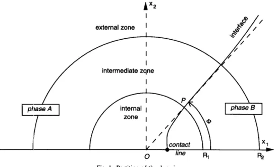
We consider a contact line moving on a plane rigid surface and we divide the domain into three parts. T h e first part, called the "external z o n e " , is the region far away from the contact line where the whole geometry of the domain and the external forces determine the flow. The classical model of capillarity can be used there. We are not interested in the flow in this region we assume that it has a weak influence upon the flow near the contact line. The second part, called the " i n n e r z o n e " , is the vicinity of the contact line; its size is so small that the thickness of the interface cannot be neglected there, the Cahn-Hilliard model has to be applied. We assume that there exists a third region called the "intermediate z o n e " close enough to the contact line for the influence of the external flow to be weak and far enough from the contact line for the classical model of capillarity to be valid. However, it is clear that external conditions may have an influence upon the behaviour of the whole interface and therefore upon the flow in the inner zone. Let us consider, for instance, the equilibrium of a small bubble lying on a plane. For a given static contact angle, the curvature of the interface depends on the size of the bubble: the shape of the interface in the inner zone depends on it. In order to get rid of this influence we assume that the curvature radius of the interface in the external zone is much larger than the characteristic size of the inner or intermediate zones.

On the other hand, in the dynamical case, a possible jump of chemical potential between the two phases in the external zone leads to a transfer of mass across the interface, i.e. a non-vanishing normal velocity on the interface. In order to get rid of this influence we assume that this normal velocity in the external zone is much smaller than the velocity of the contact

(7)

line. On these two assumptions we can study the flow near the moving contact line without considering the flow in the whole domain.

While the flow in the external zone is three-dimensional, we assume that it is two- dimensional in the inner and intermediate zones (here we assume implicitly that the curvature radius of the contact line is much larger than the characteristic size of the inner or intermediate zones), so we reduce our study to a plane perpendicular to the contact line (the plane of Fig. 1). Moreover, we assume that, in a system of coordinates tied to the contact line, the interface is not moving and the flow is stationary. In such a system of coordinates it is the boundary of the domain which is moving (with a velocity tangent to the boundary). Only the normal component (normal to the contact line) of this velocity is well defined: we can state that this velocity lies in the plane perpendicular to the contact line. We denote it Vcx~.

More precisely, we assume that (in a vicinity of the contact line) every tangent line (O, P ) to the interface intersects the boundary. Let R~ be a length much larger than the characteristic thickness of the interface and much smaller than the characteristic length of the external flow, and let Re be a length much larger than R~ but much smaller than the characteristic length of the external flow. Let us consider the tangent line (O, P) such that

IIOPII

= R~ and let us choose O as the origin of the system of coordinates (O, Xl, x2) (x~ is a unit vector tangent to the boundary and normal to the contact line, see Fig. 1). This system of coordinates is tied to the contact line. Using polar coordinates (r, 0), we define the inner zone as the set { r < R ~ , 0 < 0 < 7r} and the intermediate zone as the set {R~ < r < R2, 0 < 0 < if}. The angle (xt, OP), denoted qb, is called the apparent contact angle.

The curvature radius of the interface in the external zone is much larger than R2. We assume that this is also true in the intermediate zone, thus the interface is assumed to be near plane in this zone. In fact R~ must be large enough because we know that the curvature increases (diverges) in the classical theory of capillarity when approaching the contact line.

The following section is devoted to the study of the flow in the intermediate zone in order to obtain a boundary condition for the inner zone.

3.2 Intermediate flow

In the intermediate zone we use the classical theory of capillarity. The interface is a near plane surface and no mass transfer occurs. The two phases are homogeneous and incompressible. For the sake of simplicity we assume that their viscosity coefficients are identical (no particular difficulty should arise if different viscosity coefficients are considered).

In the plane (O, xl,x2) we use polar coordinates (r, 0) and we study a stationary two-dimensional flow in the domain @ = {0 < 0 < 7r, R i < r < R2}. We assume that two phases M = {0 > ~} and ~ = {0 < dO} with mass densities p.~ and p~ are divided by a plane interface # = {0 = ~} (see Fig. 2). The normal to # pointing into M is denoted n.

Let V.~.~, V~, r.~, and r~ be the velocities and stress tensors in each phase. Let us recall our assumptions:

(i) both phases are homogeneous incompressible fluids:

V . (V,~) = 0 in M, V . (V:~) = 0 in ~ ; (3.1)

(ii) no mass transfer occurs across the interface:

V , ¢ - n = 0 , V : , . n = 0 on •; (3.2)

(iii) both phases are viscous with the same viscosity coefficient ~. The Reynolds n u m b e r is small, so we use the Stokes equation which reads:

V. (r,~)= 0 in M, V. ( ~ ) = 0 in ~ , (3.3)

(8)

Ax

external zone I ~ / /

phaseA I

/ intecrnneal i

I

/

_tact

/

x 0 line R1 R2

Fig. 1. Partition of the domain.

(iv) the velocity and the tangential c o m p o n e n t of the stress are continuous across the interface

V<¢ = V~ on # , (3.4)

( r ~ " n), = (r:~. n), on # , (3.5)

where

II

denotes the projection to the plane tangent to the interface; (v) the no-slip condition is valid on the plane

V ~ = Vcxl, V:~ = Vcxt on 6e. (3.6)

In o r d e r to consider the possibility of a mass transfer D across the interface in the inner zone, we introduce the flow rates D~¢ and D:~ in each phase across the arcs ~ = {r = R i, • < 0 < ~} and fie e = {r = Rl, 0 < 0 < ~} (see Fig. 2):

O.~= f V<, .rid/, O ~ = I " V : ~ . n d / , (3.7)

J t J . i d ,~J', . ~

where n denotes the normal to ~<v or ~ pointing into M or ~, respectively.

/

S 0 R

/ /

S

_R2

(9)

A s a r e s u l t o f e q u a t i o n s (3.1), w e c a n u s e t h e flow f u n c t i o n s q J ~ a n d tlJ:~ s u c h t h a t , f o r e a c h p h a s e , p o l a r c o o r d i n a t e s o f t h e v e l o c i t y f i e l d s v e r i f y T h e p r o b l e m r e a d s

(V, Vo) = (

rl aY30' 03~) "

(3.8) A A t l J ~ = 0 in M , A A W ~ = 0 in ~ , (3.9) W . , = 0 o n 5 e N M , tIZ~ =

D~

o n # , (3.10) u2.~ = 0 o n ~Tfq ~ , qJ:~ = - D ~ o n # , (3.11) -

V~r

o n b ° f') M , - -

Ver

o n b ° N ~ ( 3 . 1 2 ) a 0 a 0 at-IJ ~ 4 OIJx/.q~ 321"tJ ~/ 021J~ - - - o n 5% - - - - o n # . ( 3 . 1 3 ) 00 30 002 002 T h e s o l u t i o n o f this p r o b l e m is n o t u n i q u e l y d e t e r m i n e d as n o c o n d i t i o n o n t h e b o u n d a r i e s {r = Rt} a n d {r = R2} is g i v e n . W h e n D ~ = 0 a n d D ~ = 0 s i m i l a r i t y s o l u t i o n s [ w h e n t h e f u n c t i o n s tlJ h a v e t h e f o r m W ( r , 0 ) =

rF(O)]

a r e k n o w n t o r e p r e s e n t c o r r e c t l y t h e flow in a c o r n e r [27]. W h e n V~ = 0 w e u s e r a d i a l flows [ ~ h a v i n g t h e f o r m qJr, 0 ) = F ( 0 ) ] . U s i n g t h e l i n e a r i t y o f t h e p r o b l e m w i t h r e s p e c t t o t h e p a r a m e t e r s D ~ , D ~ a n d Ve, w e o b t a i n

tlJ.~(r, O) : r[a.~

s i n ( 0 ) + b ~ c o s ( 0 ) +

c~O

s i n ( 0 ) +

d~O

c o s ( 0 ) ] + [g,~(Tr - 0 ) 2 +

h~(x -

0 ) 3] (3.14)

qJ:,(r, O) = r[a.~ sin( O) + c~O

s i n ( 0 ) +

d~O

c o s ( 0 ) ] +

[g~O 2

+ h~O 3]

(3.15) w h e r e

~ x ~ - q b ) ( s i n ( d o ) c o s ( d o ) - do) + xdo sin(do) 2

a.u = V~do - - - ~ - ) ~ ) ( - ~ - 2 ~ - ) - - s i ~ ) ' (3.16)

- ( t o - do) - sin(do)cos(do)

a:~ = Vc do(l r _ do) _ sin(do)cos(qb)(tc - 2do) - sin2(do) '

- ffdo sin(do)cos(do) + sin(do) 2

b.~ = V~ do(x - do) - sin(do)cos(do)(zr - 2do) - sin2(do) '

(3.17)

(3.18)

- do sin(do) 2

c.~¢ = V~ do(tr - do) - s i n ( d o ) c o s ( d o ) ( x - 2do) - sin2(do) ' (3.19)

(tr - do)sin(qb) 2

c:, -- V¢ do(zr - do) - s i n ( d o ) c o s ( d o ) 0 r - 2do) - sinZ(do) '

- d p cos(do)sin(do) + sin(do) 2

d,¢ = V~ do(zr - do) - sin(do)cos(do)(ff - 2do) - sinZ(do) '

( x - do)cos(do)sin(do) + sin(do) 2 d:~

V~ do(jr - dO) - sin(q~)cos(do)0r - 2do) - sinZ(do) '

(3.20) (3.21) (3.22) ,-, 3(27r - do) - 3 g.~ = u.~2---7--, _-L~rUr ~ - z 4- D , ~ - - (3.23) ' 27rdo' 3 -3(,I, + x)

g:~ = D~

27rQr - do) + D ~ 2zrdo2 , (3.24)

(10)

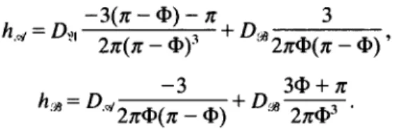
-3(~r - O) - tr 3

h~ = D,,, 21r(Tr - 0 ) 3 + D,~ 2trO(~r - O ) ' (3.25)

- 3 3 0 + ~r

h~.~ = D.~2xO(zr

_ O) + D.~ 2zrO---5-. (3.26)

This solution cannot be the physical solution for a moving interface in the vicinity of the contact line (R~ = 0) as the dissipation in any open part of the domain containing O would be infinite, and the normal stress jump across the interface would diverge when approcaching O, thus the Laplace', law binding this jump to the interface curvature could not be satisfied even approximately. However, this solution can be a good approximation for the flow in an intermediate zone (far enough from O for the normal stress jump to be small and close enough to O for the external flow to have a weak influence). We will use it in Section 4 to write the boundary conditions for the inner problem. For this purpose, we denote by Vv~'°~"°~'*(0) the velocity on ~,~ t.J ~ corresponding to W~ or W~ depending on whether 0 < • or 0 > • (the superscripts recall the d e p e n d e n c e of this boundary velocity field on the parameters

V~, D~, D:~

and 0 ) .

4. I N N E R P R O B L E M

In the inner zone the characteristic length is so small that the classical theory of capillarity is no longer valid: we cannot neglect the thickness of the interface. A non-zero thickness is fundamental because it removes the discontinuity of the mass density field, then it removes the discontinuity of the velocity field when mass transfer occurs, and finally removes the singularity of the dissipation at the contact line.

4.1 Boundary conditions

The inner domain and the expected solution are represented in Fig. 3. The domain is a half disc @n, limited by a half circle Yn, and a segment 5¢R,. n denotes the external normal to the

/

Ax2

n

~ " ~ \

'1 /

~

P //00"

/

_¢

S R 1 0 _SR1 _{x 1} Flow lines Isodensity curves

(11)

boundary. In this drawing the thickness of the interface (i.e. the zone where the isodensity curves are concentrated) was exaggerated. In fact the interface at r = R~ looks like a line in an R~-scale.

Let us discuss the static boundary conditions first:

(i) Due to our definition of inner zone (see Fig. 1), the interface intersects ZR, orthogonally. It is known from the equilibrium theory of a Cahn-Hilliard fluid ]equation (2.22)] that this condition is obtained by setting G = 0 on ZR,.

(ii) At equilibrium the contact angle ~ is connected with the value of G on 5eR, ]equation (2.21)]. This value is given by the physics of wall-fluid interactions. Fixing G is equivalent in the Cahn-Hilliard theory to fixing the static contact angle in the classical theory of capillarity.

(iii) At this point the static problem is not well-posed. We must write an extra condition deriving from the external solution. We have already discussed this point in Section 3.1 and concluded that the interface curvature should be fixed. As such a condition raises technical difficulties we prefer to fix the total amount M of mass lying inside the inner zone. The parameter M will then be adjusted to make the curvature of the interface vanish at r = R~ (therefore the interface fits with a plane interface in the intermediate zone).

Conditions (i)-(iii) lead to a well-posed static problem whose solution corresponds to a plane interface intersecting the wall at the origin with an angle compatible with Young's law. This situation is used for a first validation of the numerical simulation we describe in Section 5. It must be noted that, due to its non-linearity, this problem in general does not have a unique solution.

Let us now consider dynamical conditions:

(i) On b°R, we admit the no-slip condition V = Vcx~.

(ii) On the boundary ZR,, V coincides with a solution

V v''D.'°'°*

obtained for the intermediate zone (see Section 3.2).

As the parameters ~ , D , and D:~ are unknown (the study of • is one of our main objectives), we must write some supplementary conditions.

(iii) We deal only with mass density fields p whose variations are concentrated in a thin layer. Then we can measure the apparent contact angle (see Fig. 3 or Fig. 4) and we state that qb coincides with this angle.

(iv) As we study stationary flows, the total mass supply in

@R,

must vanish

(fx~,

P Vv~'°'D~'"*

n dl = 0), so:

D , = - [fx~,

pVV~'°'t''n*

d / I - ' [fx~, pvV~'L°'*"

ndl]D,~.

(4.1)

(v) The mass transfer from phase M to phase ~ is unknown. This uncertainty comes from external conditions (see Section 3.1). We assume that the phases are close enough to the chemical equilibrium for the mass transfer across the interface to be negligible for r-> R~. Thus D.~ will be adjusted to make mass transfer vanish at r = Rt.

These last three conditions allow us to compute the parameters ~ ,

D~

and D.,~ when the field p is known. Then, using (ii), we know the velocity field on the boundary

Zn,.

Let us sum up our boundary conditions: we write a non-homogeneous N e u m a n n condition for the mass density field p, plus a global condition upon the mass M contained in the inner zone. For the velocity field, we write a non-homogeneous Dirichlet condition which depends on the mass density field and on a mass transfer D.~¢. The two parameters M and D ~ represent the influence of external conditions upon the flow in the inner zone. A n adequate selection of these parameters will lead to a near plane interface without mass transfer at r = R~.

(12)

4.2 Equations of the inner problem, dimensionless parameters

Recalling the set of equations stated in Section 2 and the boundary conditions discussed in the previous section, the problem is to find a vector field V and a scalar field p such that:

pV( o W -

AAp] = V . (II) in DR, (4.2)

\ Op

/

V- (pV) = 0 in 9n, (4.3) V = Vex1 on 5en~ (4.4) n . V p = G o n 5¢R, (4.5) n . V p = 0 OnZR, (4.6) V = vV~'°~'°"'~'(0) on ZR, (4.7)

f

pds=M,

(4.8) RI

the parameters ~ , M, D~ and D~ being such that (i) • is the apparent contact angle;

(ii) the curvature vanishes at r = R~; (iii) no mass transfer occurs at r = R1; (iv) total mass supply vanishes.

We define the characteristic surface energy or, mass density Pd and length L by

o" = ~o dp, Pd -- 2 ' o" (4.9)

v

The length L is characteristic of the thickness of the interface and o- is the surface tension. We define the dimensionless parameters

R = R 1 Pl + P v U m - - -L ' 2/9 0 v Ca-- , K - - - o" ~:'

Gpuh

2M

- - , m = (4.10) ' g = o -

Lpo'

D~

d~ = VeL '

d~ = VeL"

(4.11)

By construction R >> 1. Far enough from the critical point u m is of order 1. g is of order 1 and fixes the static contact angle. T h e capillary n u m b e r Ca is the ratio of the viscous forces to the surface tension. It is the most important parameter.

Using the dimensionless mass density u = ( 2 p d ) - l ( 2 p - (Pl + Pv)), the dimensionless velocity

v = V~-1V and 1Lhe dimensionless free energy

w(u)= pZAo-ZW(p),

the problem (4.3)-(4.8)

reads

(U q- Um)V( ~-- Au) =GAY" (n)

V ' ( ( U + U m ) V ) = 0 i n D R V = X 1 o n 9°R n - V u = g onb°R n . V u = O OnZR v = v]'d~"d~'*(0) on Zn

f u d s = m

R

where II = K tr(D)Dd + 2D and D = ½(Vv + 7v'). in DR (4.12) (4.13) (4.14) (4.15) (4.16) (4.17) (4.18)

(13)

5. N U M E R I C A L S I M U L A T I O N

5.1 Two auxiliary minimization problems

Let p be a given scalar field in DR, and consider the following minimization problem:

- g u u (5.1)

inf w(u) - pu + ~ Vu ] ds dl; ds = m .

As w is a non-convex function, this problem in general does not have a unique solution. If u is a local minimizer of (5.1), for every 6 e H l ( ~ n ) such that f ~ 6 ds = 0, it verifies:

f~[~u(U)~-pS + Vu . V~]ds-g f~ ~dl=O

(5.2) and then Euler equations:

Ow

Ou (u) - p - Au = constant in DR, (5.3)

n . Vu - g = 0 on 6en, n . Vu = 0 on YR. (5.4)

By differentiation (5.3) implies:

V ( ~ u u ( U ) - A u ) = V p in@R. (5.5)

Now let u be a given scalar field, let qb e ]0, 7r[, de and d~ be three given parameters such that fx, (u~ + u)Vl "a'~'a.`'*. n dl = 0 and consider the following minimization problem:

inf t ( [ V v : V v + K T " ( v ) 2 ] ds} (5.6)

wX t3~s~ 2

where X = {v ~ HI(~R); V" ((Um+ U)V) = 0 in ~R, V = Xl on S~R, v = Vl 'dr''d'~''~ on ZR}. The minimizer v of (5.6) verifies the linear system of partial differential equations:

V" (H) - (u + Um)V q = 0 (5.7)

7 " ((Urn + U)V) = 0 in ~R (5.8)

v = xl on 5eR (5.9)

v = Vl ''c'a."'* on ZR. (5.10)

H e r e the field q is the Lagrange multiplier of the constraint V •((Um + u)v) = 0. It is defined up to a constant. Setting p = C,q, equation (5.7) may be written as

C a r " (II) -- (U + Um)V p = 0. (5.11)

5.2 Algorithm

It is clear from (5.8)-(5.11) and (5.4)-(5.5) that solving simultaneously problems (5.1) and (5.6) leads to a solution of the inner problem (4.12)-(4.18). Such is the principle of our algorithm:

For given parameters m and d~:

(i) we first set p = 0, solve (5.1) and get an equilibrium configuration u;

(ii) we compute the apparent contact angle qb, the value of d.~ such that the total mass supply vanishes and then we get the boundary velocity field V~"l"'l"'~';

(iii) we solve (5.8)-(5.11) and get a new field p; (iv) we solve (5.1) and get a new mass density field u; (v) then we repeat steps (ii)-(iv) until they converge;

(14)

(vi) finally we adjust parameters m and d u and repeat the whole procedure in order to have a near plane interface without mass transfer when r = R,.

Problems (5.1) and (5.6) are discretized by a finite difference method. Problem (5.10) is linear. We solve it by using a bi-conjugate gradient method. The problem (5.1) is strongly non-linear. We solve it by a steepest-descent method. We know that, in general, it does not have a unique solution. In order to find the expected solution we need to initialize the mass density field u with a field which is not too far from the solution. This is not very difficult for the equilibrium configuration and, in the dynamical case, we use as an initializing field the solution u obtained for a slightly smaller capillary n u m b e r Ca. Otherwise the most likely disaster is the inversion of the position of phases M and ~ which tends to happen when one of the phases tends to wet the boundary completely.

5.3 Dependence of the dynamic contact angle on the parameters

The dimensionless free energy w is a positive function such that w ( - 1 ) = w ( 1 ) = 0 and fl_~ ~ ( t ) dt = 1. In our simulation we use the polynomial w(u) = ~(1 - u2) 2. Such a form for the free energy is valid when the fluid is not too far from the critical point. We hope that, qualitatively, our results do not depend on the form of w.

In Fig. 4 we show the density field in a typical situation: R = 20, Um----2, K = 10, g = 0, C a - - 2 0 × 10 -3. In Fig. 5 we show the flow lines in the same situation. We notice that the curvature of the interface and the transfer of mass across the interface are concentrated in the immediate vicinity of the contact line, so the dynamic contact angle is well determined. H e r e it is about 1.9 while the static contact angle is Ir/2.

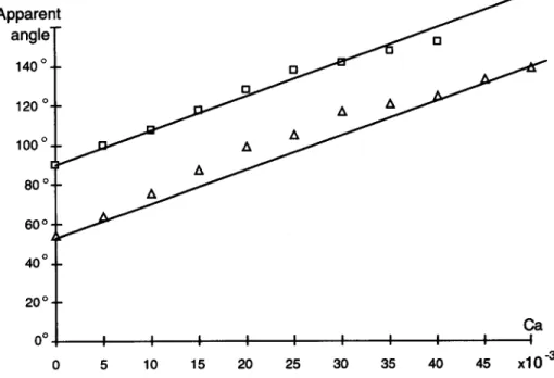
In Fig. 6 we show the d e p e n d e n c e of the contact angle on the capillary n u m b e r Ca in two cases ( R = 2 0 , u m = 2 , K = 1 0 , g = 0 a n d R = 2 0 , Um=2, K = 1 0 , g = - 0 . 3 ) . When C a = 0 t h e apparent contact angle coincides with the theoretical static angle predicted by equation (2.21), then its increase is almost linear with respect to the capillary number. The growth rate does not depend on the static angle (see Fig. 6).

We have noted a weak influence of parameter urn: the growth rate decreases slightly when Um increases. This d e p e n d e n c e can be interpreted in the following way: when approaching the critical temperature, Um increases, the difference between the mass densities of the phases decreases and the mass transfer is easier.

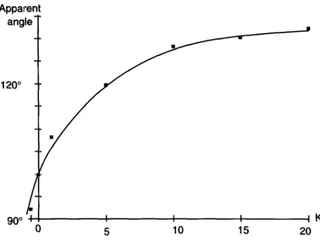
As expected, the growth rate depends strongly on the parameter K which is responsible for

(15)

Fig. 5. Flow lines in the inner zone.

mass transfer dissipation. Figure 7 shows the influence of K in the situation of R = 2 0 , /4 m ~ - 2,

g = 0 , C a = 2 0 × 1 0 -3.

6. C O N C L U S I O N

T h e C a h n - H i l l i a r d model used in this p a p e r is very simple and comparisons with experiments would be difficult. H o w e v e r , it gives an enlightening view of the flow at a contact line. First of all, mass transfer is the f u n d a m e n t a l fact which r e m o v e s the force singularity (in this connection it would be interesting to extend this study to the motion of an interface dividing two slightly mixable fluids). Secondly, it shows that the main change in the direction of the interface lies in the immediate vicinity of the contact line (the same region where mass transfer occurs). In this region the interface cannot in any way be considered a dividing surface

A p p a r e n t a n g l e ~ " 140 o =. 120 o. 100 o . 60 ° A A A A A A 20 ° 0 ° 5 10 15 20 25 30 35 4 0

Fig. 6. Dependence of the contact angle on the capillary number.

Ca

(16)

Moving contact lines

Apparent

angle" 1 2 0 ° J

l

9 0 ° I I I I I K 0 5 10 15 2 0

Fig. 7. Dependence of the contact angle on the parameter K.

991

and the classical model of capillarity cannot be applied. Thus, any study considering the interface a bidimensional surface must use a velocity-dependent contact angle: our results are in favour of model " D " following the notation and discussion of Hocking [11]. Indeed, no real angle equal to the static angle can be defined.

We found a near linear relation between the angle and the velocity of the contact line. This linear dependence gives reasonable results if there is no hysteresis of the static contact angle [8]. Indeed, there is no hysteresis in our model. The way to model contact angle hysteresis in the Cahn-Hilliard theory is to consider rough surfaces. This has not been done here (and would be incompatible with the steady flow assumption).

For a large capillary number, some problems of convergence of our algorithm arise. That is why in Fig. 6 the apparent contact angle does not reach the values ~ = 0 or • = Jr. It might be a purely numerical phenomenon. It might be connected with the non-uniqueness of the solution of (5.1); but it might also be due to the physics: a steady flow may not exist for a large velocity or a small angle. Indeed experiments (as reported in [9]) seem to point out a maximum value for the contact ~Lngle.

Our study is valid in isothermal conditions. It is also valid in adiabatic conditions (it is enough to replace the free energy E by the internal energy); but the energy transport may be the factor which limits phase transition near the moving contact line. It should be necessary to add the heat equation to our problem (4.3)-(4.8).

Acknowledgements--This research has been supported by the Centre National d'Etudes Spatiales (Contract No 92/CNES/0295) and by the Region Provence-Alpes-C6te d'Azur.

R E F E R E N C E S [1] E. HUH and L. E. SRIVEN, J. Colloid Interface Sci. 35, 85 (1971). [2] V. E. B. DUSSAN and S. H. DAVIS, J. Fhdd Mech. 65, 71 (1974).

[3] V. V. PUKHNACHOV and V. A. SOLONNIKOV, Prikl. Math. Mech. USSR 46, 771 (1983). [4] P. SEPPECHER, 10" Congrds Frant:ais de M~canique 3, 307 (1991).

[5] P. G. DE GENNES, Rev. Mod. Phys. 57, 827 (1985). [6] L. M. HOCKING, J. Fhdd Mech. 77, 209 (1977). [7] P. A. DURBIN, Q. Jl Mech. AppL Math. 42, 99 (1989). [8] P. J. HALEY and M. J. M1KSIS, J. Fhdd Mech. 223, 57 (1991). [9] Y. D. SHIKHMURZAEV, Int. J. Multiphase Flow 19, 589 (1993).

(17)

[10] C. G, NGAN and V. DUSSAN, J. Fhdd Mech. 209, 191 (1989). [11] L. M. HOCKING, J. Fhdd Mech. 239, 671 (1991).

[12] J. KOPLIK, J. R. BANAVAR and J. F. WILLEMSEN, Phys. Fhdds A1, 781 (1989). [13] P. GERMAIN, J. Mgcan. 12, 235 (1973).

]14] F. DELL ISOLA and P. SEPPECHER. Mecanica (to appear). [15] J. W. CAHN, J. Chem. Phys. 8, 66, 3667 (1977).

[16] J. E. DUNN and J. SERRIN, Arch. Rational Mech. A n a l 88, 95 (1985). [17] I. MISLLER, Thermodynamics. Pitman, London (1985).

[18] P. CASAL, C.R. Acad. Sci. Paris 274, s6rie A, 1571 (1972).

[19] P. CASAL and H. GOUIN, C.R. Acad. Sci. Paris 300, s6rie II, 231 (1985). [20] P. SEPPECHER, Ann. Phys. 13, 13 (1988).

[21] P. SEPPECHER, C.R. Acad. Sci. Paris 309, s6rie II, 497 (1989). [22] L. MODICA, Ann. Inst. H. Poincard Anal. Non Lindaire 5, 453 (1987). [23] J. W. CAHN and J. E. HILLIARD, J. Chem. Phys. 31, 688 (1959).

[24] G. BOUCHITTE and P. SEPPECHER. Motion by Mean Curvature (Proceedings) (Edited by G. B U T I ' A Z Z O and A. VIS1NTIN), p. 23. De Gruyter, New York (1992).

[25] P. SEPPECHER, Eur. J. Mech. B12, 69 (1993).

[26] G. ALBERTI, G. BOUCHITTE and P. SEPPECHER, Arch. Rational Mech. A n a l (submitted). 127] H. K. MOFFATT, Fluid Mech. 18, 1 (1963).