HAL Id: tel-01131202
https://tel.archives-ouvertes.fr/tel-01131202
Submitted on 13 Mar 2015
HAL is a multi-disciplinary open access
archive for the deposit and dissemination of sci-entific research documents, whether they are
pub-L’archive ouverte pluridisciplinaire HAL, est destinée au dépôt et à la diffusion de documents scientifiques de niveau recherche, publiés ou non,
Water balance assessment for stable water management
in island region
Seong Joon Byeon
To cite this version:
Seong Joon Byeon. Water balance assessment for stable water management in island region. Other. Université Nice Sophia Antipolis, 2014. English. �NNT : 2014NICE4106�. �tel-01131202�
UNIVERSITE DE NICE-SOPHIA ANTIPOLIS
ECOLE DOCTORALE STIC
SCIENCES ET TECHNOLOGIES DE L’INFORMATION ET DE LA COMMUNICATION
T H E S E
pour l’obtention du grade de
Docteur en Sciences
de l’Université de Nice-Sophia Antipolis
Mention : Automatique, Traitement du Signal et des Images
présentée et soutenue par
Seong Joon BYEON
Water Balance Assessment for Stable Water Management
in Island Region
Thèse dirigée par Philippe GOURBESVILLE
soutenue le 28 novembre 2014
Jury :
M. Gye Woon CHOI, Professor, Incheon National University
M. Dong Wook KIM, Professor, Incheon National University
M. Seung Jin MAENG, Professor, Chungbuk National University
M. Chang Soo SONG, Professor, Honam University
M. Philippe AUDRA, Professor, University of Nice Sophia Antipolis
The present dissertation has been approved by the
dissertation committee as a Ph. D. dissertation of
BYEON Seongjoon
February, 2015
Committee chair
Committee member
Committee member
Committee member
Committee member
ABSTRACT
Korea repeatedly experiences floods and droughts that cause traumatic environmental conditions with huge economic impact. With an approach and solution such as Smart Water Grid these problems can be alleviated. Tapping into the retention ponds behind dams, rainfall harvest facilities in urban areas and any other structures installed to store rainfall water during flood events will mitigate the damage of flooding and provide a new source of national water resources. Similarly, purified waste water, ground water and desalinated sea water can also be feasible to use as alternative water resources.
In this study, the water balance assessment model is being developed as a Smart Water Grid research. In fact, large proportions of water resources in Korea rely on river fresh water. Also in the Youngjongdo island, tap water from water purification plant which use original source from the Han river. However the water supply system in the island is quite dangerous since the water purification plant is located in Incheon city and the water comes to island through the sea and no other source is used in the island. Therefore, once the accident at main water pipe in the sea, no water is available in this island.
Information on water availability and water needs are crucial to identify hot spots of quantitative pressures on water resources. In this study, all available alternative water sources are calculated by the model developed through this study. Several physical and stochastic models on hydraulic and hydrological approaches are nominated to investigate physical characteristics of catchments.
Through this study, following results were concluded; a) To preserve the water balance in the study area, this study assessed the water balance within consideration of scenarios and suggested smart water management system which can cover potential risks on current water distribution system.; b) Within the scenario of accident on water supply system, all potential water resources in the island have been calculated through the model developed through this study. As well as, designed capacity of WWTP and desalination plant could also add self-supply
water resources.; c) The water balance in the study area was analyzed through estimation of water demand and available water resources in the study area. Although the study area is an island which the major water sources such as dams or national managed rivers are not connected to, water resources from rainfall-runoff through small streams, reservoirs and retention ponds were sufficient to cover water demand.; and d) This study suggested simple and fundamental directions to apply smart water management technologies for the island region which can cover the water for non-drinking purposes at ordinary state. And the smart water management system was analyzed as being able to counter potential problems on water supply system which causes short-term water cutting off.
Table of Contents
Abstract ··· ··· ··· i
Table of Contents ··· ··· ··· iii
List of Tables and Graphs ··· ··· ··· vi
List of Diagrams ··· ··· ··· viii
CHAPTER 1 INTRODUCTION ... 1
1.1.RESEARCH BACKGROUND ... 1
1.2.OBJECTIVES OF THE STUDY ... 16
1.3.LITERATURE REVIEW ... 17
1.3.1REVIEW ON MODELING ... 17
1.3.2REVIEW ON COMPUTATION OF DISTRIBUTED WATER RESOURCE ... 26
1.3.3REVIEW ON WATER BALANCE... 31
1.3.4REVIEW ON SMART TECHNOLOGIES FOR WATER MANAGEMENT ... 35
1.4.SCOPES OF THE STUDY ... 38
CHAPTER 2 METHODOLOGY AND THEORETICAL BACKGROUND ... 39
2.1.METHODOLOGY ... 39
2.2.THEORY FOR RAINFALL RUNOFF... 39
2.2.1INPUT DATA MANAGEMENT ... 41
2.2.2FLOW IDENTIFICATION AND DEMPROCESS ... 42
2.2.3PRECIPITATION DATA CONTROL ... 43
2.2.4ENERGY BALANCE AND EVAPOTRANSPIRATION ... 44
2.2.5BASIC RUNOFF CALCULATION ... 46
2.2.6FLOW PATH ROUTING ... 50
2.3.URBAN DRAINAGE MODEL ... 56
2.3.1DATA COLLECTION ... 56
2.3.2MODELING OF URBAN DRAINAGE ... 57
2.3.3SURFACE/OVERLAND FLOW MODEL ... 57
2.3.4PIPE FLOW MODEL ... 60
2.4.1GOVERNING EQUATIONS... 65
2.4.2RURAL DRAINAGE MODELING METHOD ... 66
2.5.PREDICTION OF WATER DEMAND ... 70
2.5.1PREDICTION OF DOMESTIC WATER DEMAND ... 72
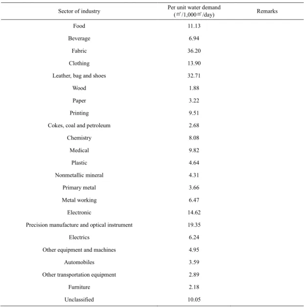
2.5.2PREDICTION OF INDUSTRIAL WATER DEMAND ... 78
2.5.3PREDICTION OF AGRICULTURAL WATER DEMAND ... 83
CHAPTER 3 DEVELOPMENT OF MODEL AND APPLICATION ... 84
3.1.GENERAL COMPOSITION OF MODEL ... 84
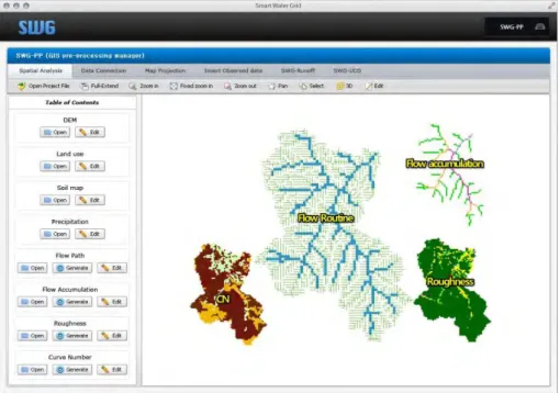
3.2.INTERFACE AND DATA COMPOSITION ... 86
3.3.DESCRIPTIONS OF MODULES ... 88
3.3.1SWG-PPGIS INTERFACE MODULES ... 88
3.3.2SWG-RUNOFF SPATIALLY DISTRIBUTED RUNOFF MODULE ... 90
3.3.3SWG-UDS OPEN CHANNEL FLOW MODULE ... 92
3.3.4SWG-DEMAND WATER DEMAND PREDICTION MODULE ... 93
3.3.5SWG-WB WATER BALANCE ASSESSMENT MODULE ... 96
CHAPTER 4 APPLYING THE MODEL AT THE STUDY AREA ... 101
4.1.STUDY AREA ... 101
4.1.1GENERAL DESCRIPTION OF STUDY AREA ... 104
4.1.2RELATIVE PROJECTS ... 107
4.1.3OFFICIAL WATER DISTRIBUTION SYSTEM ... 112
4.1.4COLLECTION SYSTEM ... 113
4.2.APPLICATION RESULTS AND DISCUSSIONS ... 114
4.2.1AVAILABLE WATER RESOURCES DATA FROM MODEL ... 114
4.2.2ADDITIONAL SOURCES FROM LITERATURE STUDY ... 118
4.2.3RESULT FROM PREDICTION OF WATER DEMAND ... 119
4.3.WATER BALANCE ASSESSMENT ... 123
CHAPTER 5 SUGGESTION OF SMART WATER MANAGEMENT PLAN FOR STUDY AREA ... 126
5.1.DEFINITION OF THE SCENARIO ... 126
5.3.WATER SOURCES AVAILABLE IN EASTERN GRID... 132
5.4.WATER SOURCES AVAILABLE IN WESTERN GRID ... 136
5.5.SMART WATER SUPPLY PLAN ... 139
5.5.1WATER BALANCE OF EASTERN GRID ... 139
5.5.2WATER BALANCE OF WESTERN GRID ... 140
5.5.3SUGGESTION OF IMPROVEMENT ON WATER SUPPLY ... 141
CHAPTER 6 CONCLUSIONS ... 151
List of Tables
Table 1.1 Characteristics of existing water balance modeling tools ... 34
Table 2.1 Mean daily duration of maximum possible sunshine hours for different months .... 45
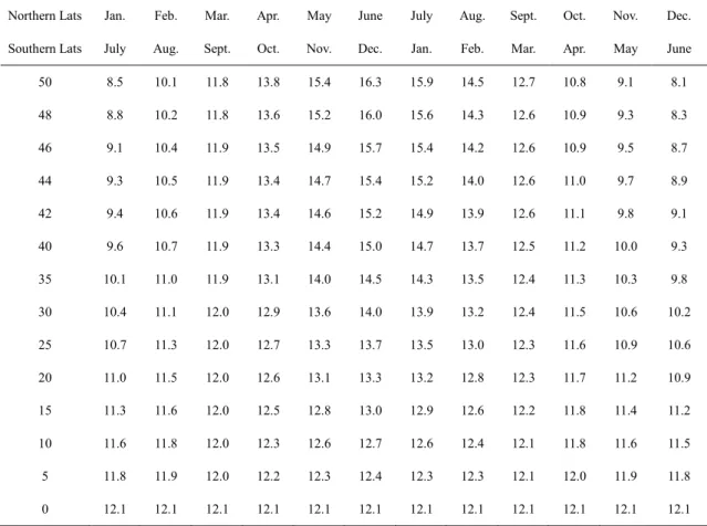
Table 2.2 Values of the weighting factor Wta at different altitudes and temperature ... 46
Table 2.3 Per unit water demand at different sector of industry ... 78
Table 2.4 Per unit water demand at different sector of industry ... 81
Table 3.1 General comparison of this model with previous models ... 85
Table 3.2 Description of necessary modules ... 85
Table 3.3 Summarize of methodologies for water demand prediction ... 93
Table 4.1 General information of villages in the Yeongjongdo Island ... 105
Table 4.2 Land use data of the Yeongjongdo Island ... 106
Table 4.3 Weather statistics in the study area ... 106
Table 4.4 Summarize of Incheon urban master plan ... 107
Table 4.5 Land use data after phase 4 of Incheon urban master plan ... Table 4.6 Population plan of the Yeongjong Sky City plan ... 109
Table 4.7 Land use plan of the Yeongjong Sky City plan ... 109
Table 4.8 The land use plan for Midan City Project ... 110
Table 4.9 Summarize of desalination plant in the Yeongjongdo Island ...111
Table 4.10 Current and planned WWTP in the Yeongjongdo Island ... 113
Table 4.11 Result of runoff modeling ... 115
Table 4.12 Result of water capacity in the reservoirs ... 115
Table 4.13 Result of capacity of retention ponds ... 116
Table 4.16 Summarize of treated waste water ... 118
Table 4.17 Potential plan for desalination plants in the study area ... 119
Table 4.18 Predicted domestic water demand ... 119
Table 4.19 Prediction of floating population and water demand ... 120
Table 4.20 Result from prediction of industrial water demand ... 120
Table 4.21 Summarize of water demand prediction result ... 121
Table 4.22 Expected scale of agricultural zone and water demand ... 121
Table 4.23 Agricultural water demand including gardening and washing water ... 122
Table 4.24 Summarize of total water demand calculated at the Yeongjongdo Island ... 122
Table 4.25 Summarize of total water resource available ... 123
Table 4.26 Scenarios of water balance assessment ... 124
Table 4.27 Water balance on scenario 2 ... 124
Table 4.28 Water balance on scenario 3 ... 125
Table 4.29 Water balance on scenario 4 ... 125
Table 5.1 Examples on accidents of submarine pipe line ... 129
Table 5.2 Basic water available at each grid ... 131
Table 5.3 Water demand at different grids ... 131
Table 5.4 Summarized table for multi water sources at each grid ... 132
Table 5.5 Simple water balance in eastern grid ... 140
List of Figures
Fig. 1.1 Common view of hydrologic cycle ... 2
Fig. 1.2 Major domains of water cycle ... 4
Fig. 1.3 Activities taking place in the various domains and water uses ... 7
Fig. 1.4 Concept of water management based on internet of things ... 10
Fig. 1.5 Concept of Water supply and demand evaluation system ... 16
Fig. 2.1 Concept of D-8 Flow grid ... 42
Fig. 2.2 Value of flow direction indicator ... 43
Fig. 2.3 The schematic diagram describing hill slope hydrology ... 47
Fig. 2.4 The schematic diagram of soil interaction of water ... 47
Fig. 2.5 Time and Space grid for numerical solution ... 50
Fig. 2.6 General procedure on urban water modeling ... 56
Fig. 2.7 Time and area curve in typical urban catchment ... 58
Fig. 2.8 Scenario A Simulation of Surface Flooding ... 62
Fig. 2.9 Scenario B Simulation of Surface Flooding... 63
Fig. 2.10 Scenario C Simulation of Surface Flooding ... 63
Fig. 2.11 Prism and wedge storage in a river channel during flood flow ... 66
Fig. 2.12 Summarized methodologies on water demand prediction ... 71
Fig. 3.1 Overall framework of modeling system ... 84
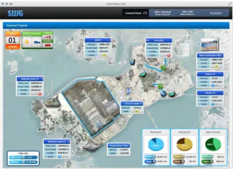
Fig. 3.2 General interface to display general result from the model Figure soon be revised. .. 86
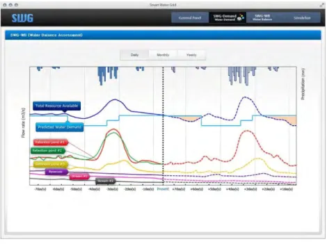
Fig. 3.3 Water balance chart interface ... 87
Fig. 3.4 Detailed information on water balance assessment interface... 87
Fig. 3.5 Spatial information data as input file of model ... 88
Fig. 3.7 Example of disagreement between different projections ... 90
Fig. 3.8 General framework of data flow and simulation ... 90
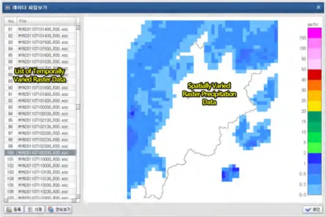
Fig. 3.9 Raster climate data ... 91
Fig. 3.10 The instant result window after the first simulation ... 92
Fig. 3.11 Description of open channel flow modeling ... 93
Fig. 3.12 Detailed information on water balance assessment interface... 95
Fig. 3.13 Methods applicable for water demand prediction ... 96
Fig. 3.14 Water balance chart interface ... 98
Fig. 3.15 System display during ordinary water cycle in the study area ... 98
Fig. 3.16 Ordinary water distribution with smart water technologies ... 99
Fig. 3.17 System display during emergency water cycle in the study area ... 100
Fig. 3.18 Emergency water distribution with smart water technologies ... 100
Fig. 4.1 Targets for system development and main task for each scale ... 101
Fig. 4.2 Comparison of candidate study area ... 102
Fig. 4.3 Potential risks on present water supply system of the Youngjongdo Island ... 104
Fig. 4.4 Villages and communities of the Yeongjongdo Island ... 105
Fig. 4.5 Map of the Yeongjong Sky City plan ... 108
Fig. 4.6 The plan map of Midan City Project ... 110
Fig. 4.7 Location map of desalination plant planned ...111
Fig. 4.8 Main pipe line of official water distribution system ... 112
Fig. 4.9 Subcatchments in the Yeongjongdo Island... 114
Fig. 4.10 Location map of retention ponds ... 116
Fig. 4.11 Location map of streams ... 117
Fig. 5.1 Conceptual diagram for smart water treatment process ... 127
Fig. 5.3 The division map of western and eastern grid in the study area ... 130
Fig. 5.4 Daily flow discharge of the Donggang stream ... 132
Fig. 5.5 Accumulated water volume of Donggang Stream ... 133
Fig. 5.6 Daily flow discharge of the Jeonso Stream ... 133
Fig. 5.7 Accumulated water volume of Jeonso Stream ... 134
Fig. 5.8 Daily flow discharge of the Unbuk reservoir ... 134
Fig. 5.9 Accumulated water volume of Unbuk reservoir ... 135
Fig. 5.10 Daily flow discharge of the East retention pond ... 135
Fig. 5.11 Accumulated water volume of East retention pond... 136
Fig. 5.12 Daily flow discharge of the North retention pond... 137
Fig. 5.13 Accumulated water volume of North retention pond ... 137
Fig. 5.14 Daily flow discharge of the South retention pond... 138
Fig. 5.15 Accumulated water volume of South retention pond ... 138
Fig. 5.16 Current water distribution system of study area ... 141
Fig. 5.17 Water distribution system as planned in 2025 ... 142
Fig. 5.18 Suggestion of smart water distribution plan... 143
Fig. 5.19 Water secure plan for emergency state ... 145
Fig. 5.20 Water balance in ordinary state at eastern grid... 145
Fig. 5.21 Broken water balance due to the accident at eastern grid ... 146
Fig. 5.22 Water balance preservation at eastern grid ... 146
Fig. 5.23 Water secure plan for emergency state ... 148
Fig. 5.24 Water balance in ordinary state at western grid ... 149
Fig. 5.25 Broken water balance due to the accident at western grid ... 149
Chapter 1 Introduction
1.1. Research Background
Korea repeatedly experiences floods and droughts that cause traumatic environmental conditions with huge economic impact. With an approach and solution such as Smart Water Grid these problems can be alleviated. Korean water resources environment is rapidly changing because of the Climate Change. For example, Rainfall pattern changed and its term became more and more concentrated. So water resources environment of Korea becomes that the rainfall of central district is increasing and southland part is decreasing. Also, some areas have problems such as water shortage and water distribution. By the way, needless to say, those who are facing the problems described above are not only Korean but it is seriously circulated as global issues. Globally, there still are more than 1.5 billion people who don’t have access to safe water and also 2.6 million people under the lack of sanitation facilities which provide clean water. Especially in the developing countries, unreliable water from poor treatment facilities causes several health problems and this problem can occasionally be linked to serious disease. There also is a problem on water itself which gradually gets polluted since the lack of treatment facilities. This is the problem coming from the unequal of water welfare.
The resources of water supply can be the water from dams, reservoirs, rivers, lakes, rainfall harvest, ground water, desalination plant, waste water treatment plant and so on and it is needless to say a lot. One more idea is making a platform to mix the water from different sources. However, only few of those sources are being used within present state although the water resources are occasionally located at outside supplying city. This is the problem of efficiency of water supply.
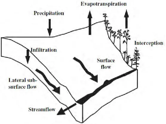
In order to figure the problem out exactly, it is firstly necessary to understand the water cycle. The water is continuously moving as definition of the hydrologic cycle which shows
movements of water throughout the earth. The hydrologic cycle which can be represented as common feature of Fig. 1.1 involves the exchange of energy, heat and the states of water [1].
Fig. 1.1 Common view of hydrologic cycle (Gourbesville, 2014)
According to the water movement through the hydrologic cycle, the total quantity of water is always constant and unlimited. Nevertheless the quantity of water as essential resource is quite limited since it is difficult to meet the quality of water for the necessary purpose within natural status. Therefore there are many activities to preserve the essential water resources and the huge domain of Integrated Water Resources Management (IWRM) concept has been developed [2]. The approach from this concept aims the maximized economic and social welfare in the equitable manners without compromising the sustainability of vital ecosystems including human by promoting the well-coordinated development and management of water resources. IWRM approaches involve applying knowledge from various disciplines as well as
the insights from diverse stakeholders to devise and implement efficient, equitable and sustainable solutions to water and development problems. As such, IWRM is a comprehensive, participatory planning and implementation tool for managing and developing water resources in a way that balances social and economic needs, and that ensures the protection of ecosystems for future generations. In such approach, ICT solutions can play a key role but focus has to be given to the most demanding and relevant domains of the water cycle. In order to identify which and how ICT solutions can be implemented, it is necessary to look at the water cycle through an approach based on functional domains and business processes. This methodology allows considering each action involved into the resource management and identifying the potential needs of ICT.
Within the concept above, the water cycle can be divided within three specific activities which are associated to activity and business domains as Fig. 1.2. The first domain is natural environment which covers conservation of water-related or aquatic ecosystem. And the second domain is natural hazards which consist of flood, water-borne disease, droughts and landslide (including avalanche events). Water disasters related to meteorological, hydrological and climate hazards repeatedly cause huge loss of life and economy. As well as, the third domain is water uses. The last domain (Water uses) covers the added influence of human activity on the water cycle. Generally, ‘water uses’ refers to the use of water by agriculture, industry, energy production and households, including in-stream uses such as fishing, recreation, transportation and waste disposal. All of those uses are directly linked to specific activities and processes which are potential targets for deployment of ICT solutions. In order to stick to the reality of the water management operated by entities in charge of water services, the traditional classification can be reviewed. The main water uses appear then as: agriculture, aquaculture, industry, recreation, transport/navigation, and urban.
Fig. 1.2 Major domains of water cycle (Gourbesville, 2014)
The detailed description about major domains of water cycle is following;
Natural environment encompasses all living and non-living things, including natural forces occurring naturally on Earth or some region thereof, providing conditions for development and growth as well as of danger and damage. It is an environment that includes the interaction of all living species. Referring specifically to water environment, there are different biotopes than can be distinguished in continental waters (rivers, lakes, reservoirs...), coastal and maritime environments. A biotope is an area of uniform environmental conditions providing a living place for a specific assemblage of plants and animals. The subject of a biotope is a biological community.
Natural Hazards mean unexpected or uncontrollable natural event of unusual intensity that will have a negative effect on the environment or people by threatening their lives or activities. Atmospheric hazards are weather-related events, whereas geologic hazards happen on
or within the Earth's surface. However, it is important to underline that atmospheric hazards can trigger geologic hazards, and geologic hazards can trigger atmospheric hazards. In the water domain, natural hazards are related to floods, droughts, tsunamis, limnic eruptions, seiche.
Water Uses are composed of the water cycle with the added influence of human activity. Dams, reservoirs, canals, aqueducts, intakes in rivers, and groundwater wells all reveal that humans have a major impact on the water cycle. According to the defined water domains, the water uses represent the largest field where ICT solutions can be developed and implemented. All in all, the Water uses considered in this framework are:
- Agriculture: Irrigation water use is water artificially applied to farm, orchard, pasture, and horticultural crops, as well as water used to irrigate pastures, for frost and freeze protection, chemical application, crop cooling, harvesting, and for the leaching of salts from the crop root zone. In fact, irrigation is the largest category of water use worldwide.
- Aquaculture: also known as aquafarming, is the farming of aquatic organisms such as fish, crustaceans, mollusks and aquatic plants. Aquaculture involves cultivating freshwater and saltwater populations under controlled conditions, and can be contrasted with commercial fishing, which is the harvesting of wild fish. This implies some sort of intervention in the rearing process to enhance production, such as regular stocking, feeding, protection from predators and so forth. It also implies individual or corporate ownership of the stock being cultivated. Similar to agriculture, aquaculture can take place in the natural environment or in a manmade environment. This activity uses part of the water bodies in order to develop activities. Aquaculture can be more environmentally damaging than exploiting wild fisheries on a local area basis but has considerably less impact on the global environment on a per kg of production basis. Industry: This water use is a valuable resource for such purposes as processing, cleaning, transportation, dilution, and cooling in manufacturing facilities. Major water-using industries
include steel, chemical, paper, and petroleum refining. Industries often reuse the same water over and over for more than one purpose.
- Recreation: It often involves some degree of exercise as well as visiting areas that contain bodies of water such as parks, wildlife refuges, wilderness areas, public fishing areas, and water parks. Some of the activities that imply the uses of water for this purpose are: fishing, boating, sailing, canoeing, rafting, and swimming, as well as many other recreational activities that depend on water. Recreational usage is usually non-consumptive; however recreational irrigation such as gardening or irrigation of golf courses belong to this category of water use.
- Energy: Derived from the force or energy of moving water, which may be harnessed for useful purposes, such as Energy production. There are several forms of water power currently in use or development. Some are purely mechanical but many primarily generate electricity. Broad categories include: conventional hydroelectric (hydroelectric dams), run-of-the-river hydroelectricity, pumped-storage hydro- electricity and tidal power. Cooling of thermo-electric plants is another essential use of water in the field of energy.
- Transport/navigation: It refers to the transport of goods or people using water as a means of transportation (on rivers as well as canals). This water use refers only to commercial transport, since recreational transports such as sailing is considered above in Recreation water use.
- Urban: Urban water use is generally determined by population, its geographic location, and the percentage of water used in a community by residences, government, and commercial enterprises. It also includes water that cannot be accounted for because of distribution system losses, fire protection, or unauthorized uses. For the past two decades, urban per capita water use has levelled off, or has been increasing. The implementation of local water conservation programs and current housing development trends, have actually lowered per capita water use. However, gross urban water
demands continue to grow because of significant population increases and the establishment of urban centres. Even with the implementation of aggressive water conservation programs, urban water demand is expected to grow in conjunction with increases in population.
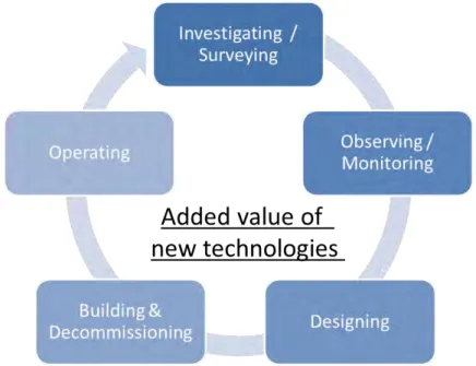
In terms of water cycle defined above, AQUA (@qua ICT for water efficiency) (2013) has described five activities for all domains of water cycle as Fig. 1.3 [3].
Fig. 1.3 Activities taking place in the various domains and water uses (Gourbesville, 2014) The first activity is investigation and survey which consist of gathering of information and data for past or present state within study domain. This assembly of information can be done either by a systematic collection of field data (survey) or a collection of information or data from a methodical research of available documents and/or the production of new ones in order to understand or to improve the actual state of the domain. The second activity is observation and monitoring. This activity, in terms of general point of view, means the awareness of the state of a system. It describes the processes and activities that need to take
place to characterize and monitor the quality and/or state of the domain in study. All monitoring strategies and programmes have reasons and justifications which are often designed to establish the current status of the domain or to establish trends in its parameters. In all cases the results of monitoring will be reviewed and analysed. The design of a monitoring programme must therefore have regard to the final use of the data before monitoring starts. The third activity is designing (or sometimes planning) which includes risk assessment. It refers the activities to meet desired needs and the process of devising a system, components and processes is mainly included. It is a decision-making process (often iterative) in which the basic sciences, risk assessment and engineering sciences are applied to convert resources optimally to meet a stated objective. Among the fundamental elements of the design process are the establishment of objectives and criteria, synthesis, analysis, construction, testing and evaluation. In order to obtain a design that achieves the desired needs for the domain in study, the two previous steps should have been accomplished and taken into account.
And the forth activity is building and decommissioning which include all activities to carry out the plans, designs or solutions proposed through the designing or planning and this activity must be carried out within consideration of risk assessment which is also proposed through the designing or planning (i.e. the third activity) to not meet the threshold of environmental impact. As well as, the fifth activity is operation which makes all designed and built system keep working as their proposed function. This activity should follow the rules designed and it may be protected and surveyed through monitoring.
We faced some points that need to make reasonable correspondence considering Climate Change within the activities and cycle above. Moreover, to secure additional headspring, mainly expand facilities were utilized, and didn't consider the Climate Change but just simply focused on the water supply system and unity water treatment system. Therefore, we need one integrated and effective water management with low-energy and high-efficiency. Smart Water Grid can make use of local IT skill with global level to solve this problem, and it can lead new generation with high green water industry which is come to the fore at water industry.
For overcoming the limitation of existing water resources management system, Smart Water Grid(SWG) appeared, which is an intelligent water management system, combined with most up-to-date technology of information and communications (ICT: Information Communication Technology). As a figure 1, through high-efficient and next generational water controlling infrastructures system, water, reused water, and seawater etc. all kinds of water sources were applied and efficiently distributed, controlled and transported. SWG is by definition the technology that water resource of regional and temporal imbalance can be effectively solved.
SWG project is to be a technology development organization that aimed at combining with Water Business (Water), Information Business (Smart) and Infrastructures Business (Grid), assuring water resources and solving the gap of water resources. It does not only assure the water quality and water safety of supplying, low energy and achieving high-efficiency, but also deal with the Climate Change. For this, the technology of assuring and distributing regional and temporal safe water resources, considering Climate Change, through the water balance assessment and automation of water supply in the area (Grid), applying the technology of water supply assessment and management, infrastructures related to ICT, assuring two ways(importing and exporting data) - real time optimal operation technology, and realizing and developing the essential technology combining with ICT integrated water resources technology.
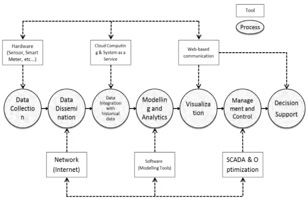
Furthermore, the applied technology can compare well with the actual place according to its own specificity, and this kind of package is expected to develop. Look into the near future, the package will be applied in the developing countries by Micro unit (Complex, Building etc.) Innovation in the Information and Communication Technology (ICT) is driven by unbroken progress in hardware performance for processing number, storing data and growing network capabilities, wired and wireless. New member in this story is the sensor for physical, chemical and biological quantities and qualities which, integrated in communication and networking, opens the door to the vision about the Internet of Things [4].
Internet of Things, in terms of original definition, refers to uniquely identifiable objects and their virtual representations in an Internet-like structure. The term Internet of Things was proposed by Kevin Ashtonin 1999. The concept of the Internet of Things first became popular through the Auto-ID Center at MIT and related market analysts publications. Radio-frequency identification (RFID) is often seen as a prerequisite for the Internet of Things. If all objects and people in daily life were equipped with identifiers, they could be managed and inventoried by computers. Tagging of things may be achieved through such technologies as near field communication, barcodes, QR codes and digital watermarking. Equipping all objects in the world with minuscule identifying devices could be transformative of daily life. For instance, business may no longer run out of stock or generate waste products, as involved parties would know which products are required and consumed. One's ability to interact with objects could be altered remotely based on immediate or present needs, in accordance with existing end-user agreements [5]. The Fig. 1.4. shows the concept of water management with internet of things.
This is seen as an integrated part of the Future Internet and might be defined as a dynamic global network infrastructure with self-configuring capabilities based on standard and interoperable communication protocols where physical and virtual “things” have identities, physical attributes, and virtual personalities and use intelligent interfaces, and are seamlessly integrated into the information network.
Transformation from the vision into some real piece of application is the idea of “Smart Water Grids” (SWG) [2] and their implementation in daily practice. A smart water grid addresses the area environment-water and is a network of fully integrated components, solutions and systems that enable a water utility to remotely and continuously;
- monitor and diagnose problems; - control and optimize reactions;
- identify and manage maintenance issues; and
- inform its customers about intelligent and cost effective usage using data-driven insight.
In a similar way smart grids might be identified in other areas such as electricity, heat, gas, transportation etc. and all these grids might interact. Sectoral smart grids may interact with grids in other areas. Best known is the “energy-water nexus” as it takes a large amount of energy to extract, treat, store and transport water. Indeed, approximately 15 to 30 percent of typical water utility’s operations and maintenance expenses are for energy. At the same time, a large amount of water is used in the production of energy - particularly as cooling water for power plants and for hydraulic fracturing or “fracking” in oil and gas drilling. This nexus will not be deepened in this paper which stays with the water- environment world.
Smart Water Grids are applications of Information Communication Technology (ICT) with the 3 main components;
- Technology: smart devices, data transmission, embedded systems, data management, online services, monitoring & control, distributed systems;
- Application: support of operation and management of systems, services for the public, service to the clients, stakeholders and citizens; and
- Market: people needs in daily life, paid & for free service.
Their development obviously must be a joint effort of specialists from different disciplines - from electronics (sensors, nets) to informatics (databases, communication), from application engineering (water-environment) to joint software system developments (information engineering), from geo- and social science to business and market with the involvement of citizens, customers, stakeholders, decision makers and politicians. Aspects of application are in the domain of “HydroInformatics” (HI) [7] which “comprehends all information technologies, methods, models, processes and systems applied in the "water-sector" and water-issues related neighbouring fields. Information is understood in an abstract sense; it may be about physics, environment, economy, social issues, organization, law, regulations and more. Models and processes concern physics, business, workflow, communication, management and more again. Thus HydroInformatics applies, generates, models, manages, transforms, condenses and archives information concerning the water-sector". So, the HydroInformatics domain, activity or movement embraces the full range of what is commonly called “business models” from public open-source developments through to private commercial developments.
In this context the role of spatial data and spatial analysis is to be mentioned as in most applications in the water-sector the basic information is related to geography, to geospatial definition of it, to its geo-localization. This means that nearly all “objects of information” are “somewhere”, and thus, benefit from very strong “Implicit Geographic Relationships” such as continuity, contiguity, inclusion, graph, neighborhood, proximity, etc. This means that the geographic approach, in a “GIS” or in a database using “geographic objects” should be the hub of the organization of HI Information Systems.
Smart Water Grids are based on the Vision about the Internet of Things. For the water-sector it is driven by eventual scarcity, growing earth population, climate change and
commercial interest. Rationally people accept this, however, smart grids by technology will change daily life of people. Do they want? Must we do everything which is be possible? This discussion starts, answers may be differently because of local traditions and cultures as what holds globally must not necessarily hold nationwide or for the region. While Korea builds its digital metropolis of smart homes in Songdo other countries are afraid of security of the nets (US). Some countries slow down implementations and Germany even says about the energy grid “it probably won’t follow smart-meter guidance from the European Union (80% of meters up to 2020) because such a move would be too costly for consumers” [8]. Nevertheless smart grid development will continue “selectively and in line with the energy switch” from nuclear to green. This puts the energy-water nexus to priority.
This market environment is an inhibitor for Large Scale Roll-out of smart water grids on the market as;
- opportunities of smart grids not known; - the water market is conservative;
- there are numerous small companies with special solutions (standards needed); - it is not clear which business partner will survive;
- it is not clear which solution will prevail;
- long-term of benefit of smart solutions is not clear; and - the risk of new technologies is not clearly addressed.
In conclusion, there is a business problem, not a technology problem.
HydroInformatics has a long tradition in the development of computational simulation software in the water-environment sector. Many of the software models are available as code for research and as packages for application on the market. These models, the expertise acquired and knowledge are available for use and platform of development towards the smart water systems. Simulation models have to be redesigned for real-time use in networks with thousands of sensors interacting. This challenge raises many technological questions about online
operation, security and reliability in water distribution networks. Smart-Online Water Distribution Network (WND) research project might serve as an example.
- Hydraulic state / flow and water quality simulation model must be extended to; - incorporate measurement, data treatment and assimilation from sensor network in
real-time to guarantee the compliance of the models with the observations. The consistency of the measurements is to be checked, methods might be Neural Networks.
- The performance of the models as well as the software design (object, agent, process oriented) have to be critically analyzed in view of high performance computing and final integration in a smart grid system. Standards have to be defined for coupling models and data.
Models have to be calibrated which for networks with thousands of sensors and transient processes cannot be done manually any more. Calibration of models must be supported by an automatic calibration framework which interacts with sensor data automatically. This task however demands knowledge about the optimal sensor distribution in a network, the sensitivity of which sensors at which location to which signal. This is also prerequisite for early warning about failure of pressure (leakage) or contamination detection. The problem of optimal sensor distribution has been covered by quite some papers during last decade, the problem mostly treated as multi-objective optimization problem.
Approaches to water quality and transport are more complicated due to physics than water quantity modeling. So the development of an online contaminant source identification toolkit would be very useful. Deterministic and probabilistic methods that were developed for offline models should be extended correspondingly.
Research on useful techniques, methods and models for this kind of research and development started many years ago in different application sectors of the water business (warning, calibration, control). Today’s methods are much advanced and technologically there
is no doubt about the feasibility of smart grids. Here HydroInformatics can help to the story a success.
Within the facing situation in several regions and solution technologies, it is needless to say that the necessary and the first element to secure water for human being is to know the water situation in the region how short it is and how to secure more water. And this study would more focus on the island region since islands easily are isolated especially in terms of water supply unless they have their own stable water source and water distribution system. A few islands which have bridges connected to inland can take water from inland but the proportion of those islands is too little. Although there are alternative water resources such as ground water, harvested rain water, desalinated sea water and so on, this type of water supply accompanies side effects with big noise pollution, high power consumption, low water quality, salt water intrusion and so on. Thus island regions occasionally face difficult to secure sufficient water and need certain assessment data to make their decision to secure water.
According to the Korean Statistical Information Service, there are more than 3,200 islands in Korea and approximately 400,000 persons are living in 470 islands [9]. This study would provide basic data to secure water for one pilot island as study area.
1.2. Objectives of the Study
This study aims the overall framework in terms of water balance assessment in the island region from the methodologies to the solutions to resolve physical and potential water shortage problems. In order to understand the definition and the application of this framework proposed through this study, it is simultaneously necessary to know about the concept of Smart Water Grid and the Hydroinformatics in terms of their theoretical approach and solution built on the basis of them. The idea in simple language, this study conducted within a part of developing Smart Water Grid and it bases on the concept of Hydroinformatics.
Then, it is necessary to make accurate assessment about water supply and demand of grid for water provision for essential market in right time and right amount. For the long term perspective, an assessment system will be developed, which can evaluate and solve water shortage of city including industrial water, agricultural water by automation technique as shown in Fig.1.5.
Tapping into the retention ponds behind dams, rainfall harvest facilities in urban areas and any other structures installed to store rainfall water during flood events will mitigate the damage of flooding and provide a new source of national water resources. Similarly, purified waste water, ground water and desalinated sea water can also be feasible to use as alternative water resources.
1.3. Literature Review
1.3.1 Review on modeling
In modelling practice there is a well-established ‘good practice’ principle within four stages [10]:
- Instantiation or set-up or ‘construction’. This consists in defining such features and parameters as discretization, computational grid, limits and boundary conditions; an introduction of topography, soil occupation, structures, initially assessed values of roughness coefficients, etc.
- Calibration, which consists in executing a number of simulations of past observed events and in varying the parameters of the model until an acceptable (to the modeller) coincidence between observations and computations is obtained.
- Validation, which consists in executing with a calibrated model a number of simulations of past observed events (different from those used for calibration) and checking to see if the simulated results are sufficiently close to observation.
- Exploitation runs (studies) with the model recognised as a validated tool.
These four stages historically come from hydrological correlative or black box modelling practice. They are a natural and indisputable approach when data-driven ‘models’ are concerned. This approach is the very essence of such ‘models’, parameters of which in most cases have no physical meaning. Such ‘models’ cannot explain what is going on within the
‘modelled’ system: they do not describe the interaction of processes within the system. What counts is the ‘training’, i.e. the calibration of these parameters in such a way that, for given inputs, computed outputs correspond to observed ones.
Many true models are in reality composed of both deterministic and data-driven or black box correlative parts. Some of the processes within the model or modelling tool may well be described by physical laws and equations but others, within the same model, may not. The MIKE SHE modelling tool provides a deterministic approach for all processes of water transfer through a catchment, but it allows the user to replace some of the deterministic components by others that are of a datadriven type. This option is often used when there is no need for some components to be predictive. A similar situation arises for other applications:
- Modelling river floods often involves a model that is a combination of a deterministic component of river flow simulation and of a data-driven rainfall/runoff component (e.g. MIKE11 and NAM).
- Modelling pollutant fate in groundwater flow often involves deterministic components, such as the water flow itself and the advection–diffusion of the pollutant, but also data-driven ones, such as the adsorption of the pollutant in unsaturated zones.
- etc.
Clearly, in all such cases the data-driven components have to be calibrated (‘trained’) as explained above. And it is important to realize that they must be calibrated separately from the overall tool and, hence, there is the need for data that concerns only these components, as well as the methodology to calibrate them as specific components. It is not easy to calibrate some components as data-driven models and then consider others as deterministic ones! However, we still have to do so with a model in the sense that we can always trace an expressive property or meaning to the productions of the tool concerned.
When we consider, however, deterministic modelling (based on physical laws describing simulated processes and their interactions), this four-stage paradigm is not only illusory as a
way of increasing accuracy but it may also lead to dubious and unreliable results. Hence it should be abandoned and a modified paradigm is to be applied when physically based deterministic models are concerned. More precisely, the calibration stage should be eliminated from the paradigm while the validation stage, as compared to current practice, should be carried out in a different way and in a different spirit. We shall illustrate this position in the following and by examples of current practice.
When the calibration of deterministic models (or deterministic components of models) is considered, one may ask oneself: what is to be calibrated? What is modified during the calibration procedure? An obvious principle (often violated in practice) is that the calibration must be limited to the model parameters that are invariant between the instantiation and exploitation stages, unless the purpose is to study the sensitivity of the model to modifications in its parameters. To calibrate parameters that will subsequently be modified during the exploitation runs used for simulating the impact of future projects is most often a useless, as well as costly, exercise. It is better by far to let a model be truly deterministic, i.e. a model without ‘inner black boxes’ describing physical processes, the only parameters of which are empirical or experimental coefficients related to physical characteristics. For example, in open channel flows in rivers, such parameters are roughness Manning/Strickler/Chezy coefficients, singular head-loss coefficients and discharge coefficients of structures (weirs, gates, culverts, etc.). But certainly not topography, dyke elevations, operations rules for structures, etc. Roughness coefficients are invariant parameters between calibration and exploitation stages, unless the exploitation concerns projects that could modify them.
Cleaning up and dredging a badly maintained river stretch invaded by vegetation will necessitate the modification of the roughness coefficients. In this situation, roughness coefficients cannot be invariant. In order to study the impact of cleaning, one may wish to calibrate the current coefficients (before cleaning) in order to ascertain that the model reproduces the present conditions accurately. But to assess the impact of the change one has to modify the coefficients for the future situation and there is no way to calibrate these new values:
they are defined through an engineering assessment. Any calibration of ‘global’ head-loss coefficients along a stretch including features, the characteristics of which vary between a calibrated situation and exploitation runs (structures, sills, narrowing or widening of the river bed, etc.), may lead to a nonpredictive black box model.
Another question to be asked and considered: in practice, is a meaningful calibration possible? It should be clear that the answer is negative, at least for most cases, because of the lack of appropriate data, or the cost of their acquisition. It can be shown in examples how ‘obvious’ applications of a paradigm including calibration may well lead to serious errors because of the belief that calibration is meaningful or because of a wrong choice of calibrated parameter. One problem area is that of open (sea) boundary conditions for two-dimensional tidal estuarine models, as introduced earlier. There are still modelers who impose tidal free-surface elevations at open boundaries and ‘calibrate’ roughness coefficients within the model using stage hydrographs recorded at a few shore stations. However, as explained earlier in this paper, water elevations within the modelled area, both in reality and in the model, follow the variations of the boundary elevations, which means that even large variations in roughness coefficients of the model have little influence on elevations that are compared with observed values. As mentioned before, the main parameters that are calibrated to make models of this kind reliable are the variation of in-flowing and out-flowing discharge hydrographs and their distribution at the open seaward boundary [11]. Roughness coefficients within the domain must be assessed using the engineering experience of the modeler and then they can only be modified rarely and only locally. It is legitimate to calibrate the discharge distribution at an open sea boundary of a tidal model for the ‘project tide’ because the same distribution and the same ‘project tide’ would be applied to exploitation runs: this distribution is invariant for the model. It is futile to do so if projects proposed for the estuary could influence the discharge distribution at the boundary.
Another classic example concerns one-dimensional river modelling. One-dimensional models of rivers have a typical resolution of computational grids between 100–1,000 m, with distances between gauging stations where the water stages are recorded being of the order of 10
000 m. Thus along a 50 km channel there might be four calibration sections (boundary conditions excluded). In open channel flow engineers can evaluate values of roughness and head-loss coefficients by inspection, within a narrow range of error. If a visual inspection of the river stretch suggests a Manning coefficient of 0.03, it is easy to accept that the actual value of the coefficient may vary between, say, 0.025 and 0.035. If, however, the calibration of roughness (coincidence between computed and observed water stages at gauges at a distance of some 10 000 m) leads for this reach to values such as 0.04 or 0.05, this is unacceptable. Indeed, such a river bed would be, according to the Strickler formula, covered with equivalent roughness elements of diameters 0.78 or 3.00 m high! The only possible conclusion in such a case is that the model does not reproduce reality and that the calibration is meaningless. Obviously, when instantiating the model for this case, something has been forgotten: a bridge, a singular head loss, river shape-induced head losses, the appropriate representation of an inundated plain, etc. Another possibility is that the river geometric characteristics are not correct in the model and calibration gives absurd values because it compensates for narrows or for sills that influence more the surface elevations than does the roughness. Or, worst of all, the model is based on equations that do not describe adequately the physical process, such as fixed-bed equations applied to alluvial bed rivers, or a diffusive wave equation model applied to downstream-influenced or inertia-dominated flows. At any rate, from the point of view of prediction and future exploitation, the calibration effort is futile and useless.
Other typical examples of meaningless ‘calibration’ (should we say mindless ‘fitting’?) of parameters until a coincidence between computed and observed free-surface elevations is reached are:
- Two-dimensional modelling of inundated plains. Indeed, the only past-observed data concerning the unsteady evolution of water stages that can be found on inundated plains are those rare marks of the highest elevations attained during historical floods. The only one known to the author, and a never repeated historical case, where the records were adequate for calibration purposes of such a situation was in the case of
the Mekong Delta Model [12][13]. There were 350 computational points and three consecutive floods (1963, 1964 and 1965) were recorded at 300 gauges located over the modelled area. The cost of the modelling and measurement campaigns was over US$1 million (at 1963 values: this would be ten times more in 2002). This number alone shows that this approach would not be repeated today.
- Two-dimensional modelling of tidal coastal areas, for the same reason: the records are available at only a very few stations, generally located at the coast where conditions are specific and the tide is deformed. Thus the calibration of large areas through fitting computed and observed results may well be meaningless because the calibration criteria for large domains are really dependent upon the local effects of features located near stations.
- Groundwater flow modelling provides several flagrant examples, of which there is only space here for one. Following the current ‘good practice’ paradigm the permeability coefficients are systematically calibrated to obtain a coincidence between observed and computed evolutions of piezometric levels. In practice, the resolution of the network of piezometric recording wells, as compared to the resolution of computational points over the modelled domain, is always very small. It is rarely dense enough to make it certain that it ‘captures’ the possible main variations of geological conditions and of permeability parameters over the domain. Consider, on the other hand, the duration of the measurement period (at best 10 years) as compared to the time needed for the flow to cross the modelled area (often 50-100 years). The chances are great indeed that the modeler, by calibrating the parameters on the basis of 10 year records, ‘twists the arm’ of reality, and that the resulting ‘calibrated’ model is not a reliable image of reality at all. Once more the calibration is meaningless.
Why then, in the current paradigm, is calibration considered as a necessary step? There are several reasons, such as:
- The end user’s or client’s measure of satisfaction. How does she or he know that the model is correct? Answering that the calibration reproduced past-observed results accurately makes him or her happy because, in the absence of any understanding of the inner mechanisms of the modelling he or she is reassured by the image of two coinciding curves.
- The end user (or client) might have spent a lot of money on collecting data, carrying out measurements, etc., and does not like the idea that this money was spent for nothing. It makes him or her happy to show that this data is being proved useful for the project: ‘these data were essential for a calibration that in turn is essential for proving the accuracy of the model . . .’.
- Suppose problems arise with a project built on the basis of modelling studies where nature did not behave as the model predicted. Then a modeler has arguments in his favour if he followed ‘good practice’ and if the calibration was carried out which led to the coincidence of past-observed and computed results.
In most specific cases, as developed above, it can be shown that these reasons are fallacious. To take a very crude intellectual shortcut, one may attempt to say that the calibration is still a common practice because it makes both sides happy: the modeler (who may estimate his or her intellectual effort as finished when the model is ‘calibrated’) and the end-user/client who feels that his or her duty of control and supervising has been done. Neither realizes that their satisfaction is so often related to a formal coincidence and not to any understanding of the physical problems, with this last criterion as the most important point for projects and future developments, and the very reason for commissioning the model at all. This is to say that the technology in such a case is not directed to an understanding of the underlying phenomena, but only to persuading an end-user or client that something of value has been done. It thus corresponds to the technologies of persuasion in their most negative sense [14].
- Instantiation or set-up or ‘construction’ of the model; definition of the methodology necessary to define the range of uncertainty in the results of the computations.
- Validation, which consists of executing a number of simulations of past-observed events with the model, computing or otherwise finding the range of uncertainty for the results and analyzing and finding physically logical reasons for differences between the simulated and observed results. After this, analyzing the impact of the differences as well as of the uncertainties upon the exploitation results.
- Exploitation runs (studies): supplying the results and impacts and their range of uncertainty to the end-user or client in a comprehensible form.
The modified paradigm for deterministic modelling as proposed above eliminates the calibration stage as such. The validation stage is not only maintained, but reinforced. In a way it incorporates the calibration stage. The past measured data will, of course, be as useful and as necessary as for calibration under the currently admitted paradigm but they will be used for a validation analysis of the computed results. It is claimed that a deterministic model, with values of parameters defined by inspection on the basis of engineering practice, should simulate reality correctly and its results should be close to past observed results without calibration in its irrational sense. ‘Close’ does not mean an immediately satisfactory coincidence. But making computed results nearer and nearer the observed ones must not be carried out through a calibration process as it is currently understood and applied. Indeed:
- If the differences between the computed and the observed lie within an acceptable interval of uncertainty, or can be explained by physical reasons, and if the consequences of differences upon exploiting the model as it is are analyzed and acceptable, then there is no reason to go any further with the modification of parameters.
- If the differences are greater than the uncertainty interval, than they must be explained. The reasons must be found and analyzed, taking into account, once more, the
consequence of using the model as it is or amending it. Most often the findings lead to modifications of originally erroneous data, such as topography, hydraulics characteristics or boundary conditions, and have not much to do with parameters. Sometimes there are factually important errors in values of parameters assessed during a visual inspection. But, sometimes, one may find that the modelling tool is not adequate: such often occurs when using 1D models where only 2D can simulate the real flows.
The new paradigm insists on the fact that this modified approach is not a calibration under a new name. The new ‘good practice’ asks for the collection and analysis of data for the purpose of validation, and validation is not just a check that computed values are not very far from observed ones: it is a study of the reasons why there is a difference between the two! Also it must, of course, be substantiated by a report leading to an understanding how such an analysis was carried out and how the conclusions were reached.
Paramount to the successful acceptance of this modified paradigm by the engineering profession as ‘good practice’ are the following conditions:
- A broad understanding of the difference, with respect to calibration, between deterministic and data-driven or black box models. A clear understanding of the difference, within a model, between an empirical parameter and a black box replacing a process.
- An acceptance that the simulation results of past events do not reproduce exactly the on-site measurements. A requirement for an engineering analysis of the differences. - An acceptance, and even a requirement, that the results of models should be presented
as uncertain and with a sound evaluation of the uncertainty range or interval.
The need for this new approach, and for this modified paradigm, is not fully recognized and not yet instituted as good practice, but the first descriptions of and information on
applications and studies that follow these ideas are beginning to become available. One such study is the modelling of flood propagation across an inundated plain in South-Western France [15]. Interested readers are encouraged to read this reference. The case is interesting precisely because a calibration, in the usual sense, would be meaningless. The link between the requirements put on the reliability of the results, on the one hand, and the means necessary to analyze and ensure an accessible degree of reliability, on the other hand, is described. It is worth noting that, even in this case the authors thought it useful to insert one paragraph titled ‘Model calibration’, although there was no calibration in the traditional sense [10][16].
1.3.2 Review on computation of distributed water resource
The water is seen the premier constitutive factor of human being. Thus, it always plays an important role to the development of human society. However, water distribution is not equal due to time and space. These unbalances conduct many negative impacts to the human. Annually, natural disaster related on water issue such as flood, drought, storm…bring out lots of severe damages. These are not only on the property but also on the life. According to IPCC (2007) in recent years, under the impact of climate change, the consequences of flood, drought catastrophes are more serious [17]. Getting the deep knowledge on the hydrological factors in a catchment is an essential objective of hydrologist community to be able to transform disadvantages to advantages or mitigate the natural catastrophic damage to people. Nowadays, with the development of mathematics and computer science, the simulating the hydrological cycle for catchment becomes easier and more accurate. These progressions help hydrologists might have concrete and truthful insights about what happens in hydrology to make good decisions for reducing natural hazards on the catchment [10].
Up to date, many hydrological models have been developed with different theories to simulated catchment’s hydrological phenomenon. They may be classified according to the description of physical process as conceptual and physical based, and according to the spatial
and inconveniences for simulating the hydrological process. Lumped models are one of simple hydrological model which assume that all characteristics are constant across the catchment such as HBV model, MIKE11/ NAM Model, Tank, Topmodel, Xinanjiang [19]. Lumped parameter models are much simpler in their treatment of spatial variation, which each model parameter described by a value that is uniform for the whole catchment so these could not be determined directly from physical characteristics of the catchment under consideration. These parameters are generally determined via calibration [19][20]. In contrast, distributed model is constructed on dividing catchment into sub units which each unit represents all physical characteristics for a real area. These kinds of models maintain the physical details at a given grid size and consider the distributed nature of hydrological properties such as soil type, slope and land use [21][22]. In principle, parameters of distributed model could be gotten from the catchment data. For this reason, distributed model is evaluated to be able to translate more accurately and concretely the hydrologic process in a catchment. One more advantage of distributed model is that the outputs such as water level, discharge, hydrological factors could be perfectly extracted at anywhere in the catchment. These efficiencies help to overcome difficulties in lack of observed data, which have a great significance for simulating the hydrological process at a large catchment or in developing countries. However, which model is the best to simulate hydrological process? Until now this question has not been clearly answered yet. There are some arguments on the advantage and limitation of this both kind of model. Even if distributed model have drawbacks on computation time, initial parameter definition or lack of spatial data for set up model as well as validation, most of modelers estimate highly the capacity of distributed model than lumped model [23][24]. The lumped models, in many case, perform just as well as distributed models with regard to rainfall runoff simulation when sufficient calibration data exist [25][26]. Conversely, the distributed model could not prove completely its performance in simulating the hydrological factor. Because the spatial input data such as topography, soil type, land use nowadays might be available to build the model, but it is really not easy to find the spatial data for calibration or validation. This leads to quality estimation of the model in the whole
catchment is mostly unable, the calibration and validation are generally carried out against the data at several gauging stations. One more weak point of distributed models is that this model type commonly consists of more parameters than lumped models so the calibrated process is more complicated and difficult to achieve the acceptable values [27]. However, Refsgaard noted that more detailed physically base and spatially distributed models are assumed to give a detailed and potentially more correct description of the hydrological process in the catchment whereby might provide more accurate predictions [21]. From these preeminence, many distributed models have been developed and applied in recent years such as MIKE SHE, SWAT, SWIM, LISFLOOD and WETSPA.
In many current hydrological models, deterministic distributed model is likely to have more advantages. The main interest of a deterministic distributed hydrological model is to be able to provide hydrological data at any locations within the catchment. This possibility allows to investigate, in depth the hydrological dynamic. Several tools are today available and could be used for such analysis. The typical model is MIKE SHE developed and extended by DHI Water & Environment since the last decades of the 20st century. MIKE SHE covers the major
processes in hydrologic cycle and includes process models for evapotranspiration, overland flow, unsaturated flow, groundwater flow, channel flow, and their interactions. Each of these processes can be represented at different levels of spatial distribution and complexity, according to goals of the modeling study, the availability of field data and the modeler's choices [28]. The representation of catchment characteristics and input data is provided through the discretization of the catchment horizontally into an orthogonal network of grid squares. In this way spatial variability in parameters such as elevation, soil type (soil hydraulic parameters), land cover, precipitation and potential evapotranspiration can be represented. Within each grid square, the vertical variations in soil and hydro geological characteristics are described in a number of horizontal layers with variable depths. Lateral flow between grid squares occurs as either overland flow or subsurface saturated zone flow. The one-dimensional Richards' equation
![Table 2.2 Values of the weighting factor Wta at different altitudes (levels) and temperature Level [m] Temperature [°C] 2 4 6 8 10 12 14 16 18 20 22 24 26 28 30 32 34 36 38 40 0 0.43 0.46 0.49 0.52 0.55 0.58 0.61 0.64 0.6](https://thumb-eu.123doks.com/thumbv2/123doknet/14533495.723826/59.892.133.767.187.364/table-values-weighting-factor-different-altitudes-temperature-temperature.webp)