© 2004 Biometrika Trust Printed in Great Britain
Posterior probability intervals in Bayesian wavelet estimation
B C. SEMADENI, A. C. DAVISON
Institute of Mathematics, Swiss Federal Institute of T echnology, 1015 L ausanne, Switzerland
claudio.semadeni@a3.epfl.ch anthony.davison@epfl.ch
D. V. HINKLEY
Department of Statistics and Applied Probability, University of California, Santa Barbara,
California 93106-3110, U.S.A.
hinkley@pstat.ucsb.edu S
We use saddlepoint approximation to derive credible intervals for Bayesian wavelet regression estimates. Simulations show that the resulting intervals perform better than the best existing method.
Some key words: Bayesian thresholding; Discrete wavelet transform; Mixture distribution; Nonparameter regression; Saddlepoint approximation.
1. I
Nonparametric estimation of a function or signal g from a data vector y=(y
1, . . . , yn)T satisfying y
i=g(ti)+ei (i=1, . . . , n), (1)
where the e
i are independent normal random variables with mean zero and variances2, may be based on procedures such as spline smoothers, kernel smoothers, local polynomial regression or wavelets. In this last approach, the noisy data are expressed as a linear decomposition in a wavelet basis, which is then usually denoised by a thresholding procedure which extracts significant coefficients and reduces insignificant ones to zero. The choice of thresholding rule is crucial, and among the possibilities are the minimax approach (Donoho & Johnstone, 1994, 1995), multiple hypothesis testing (Abramovich & Benjamini, 1995) and Bayesian approaches (Abramovich et al., 1998). Uncertainty measures for the underlying functions have been discussed by authors including Picard & Tribouley (2000) and, from a Bayesian viewpoint, Chipman et al. (1997), in addition to the work cited below.
In this paper, we focus on attaching credible intervals to the Bayesian point estimates proposed by Abramovich et al. (1998). The BayesThresh method gives a posterior distribution for each wavelet coefficient, which is then estimated by the median of its posterior distribution. The signal is in turn estimated through the inverse discrete wavelet transform. In an unpublished University of Bristol technical report, S. Barber uses simulation to obtain credible intervals for the underlying signal, whilst Barber et al. (2002) approximate its posterior distribution using Johnson curves and the first four posterior cumulants. Here we investigate the use of saddlepoint approximation to the full posterior distribution.
498
C. S, A. C. D D. V. H
We outline relevant aspects of wavelet regression in § 2, and then in § 3 derive the saddlepoint approximation of the posterior distribution of g(t
i). Numerical results are given in § 4 and some concluding remarks made in § 5.
The R code to compute our SBand posterior credible intervals may be downloaded from http://statwww.epfl.ch.
2. B 2·1. Wavelet regression
Wavelets provide multiple orthonormal bases of L2(R), the space of square integrable functions on the real line R. Using a scaling function w(t) and an associated wavelet y(t), a function g(t) in L2(R) can be represented as g(t)= ∑ kµZCj0,kwj0,k(t)+ ∑ 2 j=j0 ∑ kµZDj0,kyj0,k(t), (2) wherew
j,k(t)=2j/2w(2jt−k) and yj,k(t)=2j/2y(2jt−k) are dilations at level jµZ and translations at location kµZ of the scaling function and associated wavelet respectively. The coefficients of the representation are
Cj0,k=∆wj0,k(t)g(t)dt and Dj0,k=∆yj0,k(t)g(t)dt. Wavelet systems are good expansion sets for a variety of signals, including those with jumps, high frequency events and other nonsmooth features, and with features which change over time. Smooth portions of g(t) are represented by a small number of coarse level coefficients, whilst inhomogeneous features are represented by coefficients at finer scales. Daubechies (1992) and Chui (1992) give detailed expositions of the mathematical aspects of wavelets.
The properties of the wavelet decomposition make a discrete version of (2) an attractive basis for estimation of g(t) when only noisy observations (1) are available. In common with most other authors, we suppose that t
i=i/n and that g(t) is periodic at the boundaries. Let g denote the vector ( g
1, . . . , gn)T, where gi=g(ti), and write the observation vector y as g+e. The discrete wavelet transform of y is d*=W y=W g+W e=d+e*, where W is a n×n orthogonal matrix determined by the chosen functionsw(t) and y(t), d*=(c*
0,0, d*0,0, . . . , d*J−1,2J−1)T is the n×1 vector of empirical wavelet coefficients, d=W g is the discrete wavelet transform of g, and orthogonality of W means thate*=W e has the same distribution as e.
The inverse discrete wavelet transform would reconstruct y by multiplying d* by W−1, though the fast pyramid algorithm of Mallat (1989), which presupposes that n=2J for some integer J, is much faster than matrix multiplication. Better estimates of g are obtained by threshold rules, which extract large wavelet coefficients and set small ones to zero, and then apply the inverse wavelet transform to the resulting modified coefficient vector, yielding an estimate g@
i of gi. Perhaps the best-known approach to this was suggested by Donoho & Johnstone (1994). Bruce & Gao (1996) gave approximate confidence intervals for g@
i using the asymptotic normality of g@i, proved by Brillinger (1996) under certain conditions.
2·2. Bayesian procedures
Bayesian procedures for wavelet regression involve priors on the coefficients c0,0and d
j,kwhich are updated by the observed coefficients of the discrete wavelet transform, c*0,0and d*
j,k, to obtain posterior distributions of d
j,kand of c0,0. Bayesian point estimates c@0,0and d@j,kcan then be computed and used with the inverse discrete wavelet transform to estimate g. Some authors also place priors on s2, but we shall suppose that this can be estimated well enough to be regarded as constant.
To incorporate the assumption that only a few coefficients contain the main part of the signal, most Bayesian procedures use mixture distributions as priors (Chipman et al., 1997; Holmes & Denison, 1999; Vidakovic, 1998). The thresholding method BayesThresh (Abramovich et al., 1998) is obtained by placing a noninformative prior distribution on the scaling coefficient c
independent prior distributions on the wavelet coefficients, d
j,k~pjN(0,t2j)+(1−pj)d(0) ( j=0, . . . , J−1, k=0, . . . , 2j−1), (3) where 0∏pj∏1,d(0) represents a point mass at 0 and the d
j,k are independent. This is a special case of the normal mixture suggested by Chipman et al. (1997).
The hyperparameters of (3) are assumed to have the formt2j =2−ajC
1and pj=min (1, 2−bjC2), where C
1, C2,a and b are nonnegative constants. The first two are chosen empirically, but a and b should be chosen according to any prior knowledge of the smoothness of the unknown function g. Abramovich et al. (1998) showed that the default choicea=0·5, b=1 is robust to varying degrees of smoothness of g.
The noninformative prior placed on the scaling coefficient c
0,0leads to a N(c*0,0, t20) posterior distribution, where c*
0,0 is the observed coefficient. The posterior distribution of the wavelet coefficient dj,kconditional on d*
j,kis the mixture w
j,kN(d*j,kr2j,s2r2j)+(1−wj,k)d(0), (4)
independent of other coefficients, where r2
j =t2j/(s2+t2j), wj,k=(1+jj,k)−1 and j j,k= 1−p j p j (s2+t2j)D s exp {−r2jd*2j,k/(2s2)}. (5)
The posterior mean, which is the traditional Bayes rule, does not provide a thresholding rule, but shrinkage. Instead, Abramovich et al. (1998) suggest using the posterior median of d
j,kas the point estimate d@
j,k, yielding an implicit level-dependent thresholding rule.
The Waveband procedure of Barber et al. (2002) uses cumulants to derive credible intervals for the wavelet regression estimates. They express the first four cumulants of the posterior distribution of the estimates in terms of the observed data and integer powers of the mother wavelet functions, and approximate these by linear combinations of wavelet scaling functions at an appropriate finer scale. They find the posterior cumulants for any given dataset by a suitable modification of the discrete wavelet transform, and finally use Johnson transformations to obtain the credible intervals. The availability of the posterior cumulant generating functions of c
0,0and the dj,k, however, implies that a potentially more accurate approach is available through saddlepoint approximation.
3. S
Saddlepoint approximation enables highly accurate approximation to the density or distribution function of a random variable X through its cumulant generating function K(u) (Daniels, 1954, 1987; Jensen, 1995; Reid, 1988; Davison, 2003, Ch. 12). Recall that K(u) is defined as log M(u), where M(u) is the moment generating function of X, assumed to exist in an open set containing u=0, and that the rth cumulant is defined to be the coefficient of ur/r! in the series expansion of K(u). Elementary properties of moment generating functions imply that the cumulant generating function of a linear combination X=Wk
l=1clXlof independent random variables X1, . . . , Xkwith cumulant generating functions K
1(u), . . . , Kk(u) is K(u)= Wkl=1Kl(clu).
The cumulative distribution function F(x) of X at x may be approximated by FB (x)=W
C
v 1(x)+ 1 v 1(x) logq
v2(x) v 1(x)rD
, (6)whereW denotes the standard normal distribution function and v
500
C. S, A. C. D D. V. H
the saddlepoint uA =uA(x) satisfies K∞(uA)=x, and K∞(u) and K◊(u) are the first and second derivatives of K(u) with respect to u. Typically these formulae are used to approximate the cumulative probability corresponding to a specified x, by solving the equation K∞(u)=x iteratively to give the corresponding saddlepoint uA(x), and then computing (7) and (6). When the entire distribution or its quantiles are needed, however, iterative root-finding can be avoided by noting that, if u is specified, then K∞(u) and K◊(u) are easily obtained, giving x=K∞(u); the corresponding FB(u) is found using (6) and (7), so no root-finding is required. This direct computation of pairs (x, FB (x)) is performed for a grid of values u
1, . . . , uSof u, yielding values x1=K∞(u1), . . . , xS=K∞(uS) of x and their cumulative probabilities FB (x
1), . . . , FB (xS). Approximate quantiles of F may be obtained by interpolation among x
1, . . . , xSas functions ofW−1{FB(x1)}, . . . ,W−1{FB(xS)}, using for example a spline smoothing routine. In many cases it suffices to take S=20 equally-spaced values of u in the range ±3·5K◊(0)−D, though more sophisticated adaptive strategies are possible.
We now discuss how this approach may be used to obtain approximate posterior quantiles of g i given the data. The first step is to obtain the posterior cumulant generating function of g
i. Without loss of generality, we assume that the noisy signal y has been centred to have average zero. If so, the scaling coefficient c
0,0of the discrete wavelet transform is zero, and the wavelet representation of g i=g(ti) is g i= ∑ J−1 j=0 ∑ 2j−1 k=0 d j,kyj,k(ti) (i=1, . . . , n), (8) where the d
j,k are the wavelet coefficients. Equation (4) implies that these are independent a posteriori, so the posterior cumulant generating function of g
iis K
gi|y(u)= ∑j,kKdj,k|y{uyj,k(ti)} (i=1, . . . , n), (9) where
K
dj,k|y(u)=log {wj,kexp (ud*j,kr2j +u2s2r2j/2)+1−wj,k}. (10) The calculation of (9) requires the values ofy
j,k(ti) andy2j,k(ti) for all ti, j and k. Except for a few special cases, wavelet functions have no analytic form, so Barber et al. (2002) approximate powers of wavelets using weighted sums of appropriately shifted scaling functions. We avoid the numerous approximations that this entails by the following procedure. For given jA and kA, we set all coefficients of d=(c
0,0, d0,0, . . . , dJ−1,2J−1)T to zero, except for djA,kA which is set to 1, and we then apply the inverse discrete wavelet transform to d using the wavelets of interest. The resulting signal is a vector of n values corresponding to the vector (y
jA,kA(t1), . . . ,yjA,kA(tn))T. This procedure can be performed for all wavelet functionsy
j,k(.), and it returns the values of these functions at each ti. With these refinements, the approach described above can be applied to (9) and yields approximations to any required posterior quantiles of g
1, . . . , gn.
4. N
We used simulation to assess the performance of our procedure SBand and compare it with WaveBand (Barber et al., 2002). We took the ‘Blocks’, ‘Bumps’, ‘Doppler’ and ‘Heavisine’ test functions of Donoho & Johnstone (1994), and the piecewise polynomial ‘Poly’ of Nason & Silverman (1994), all rescaled to have unit standard deviation. One thousand simulated data-sets with n=1024 were created by adding noise with mean zero and root-signal-to-noise ratio r=4; this is the ratio of the standard deviation of g(t
1), . . . , g(tn) to the standard deviation of the noise. The SBand and WaveBand credible intervals for the same 1000 noisy signals were
evaluated at each data point for nominal coverage probabilities 0·90, 0·95 and 0·99. Both methods used Daubechies’ least asymmetric wavelet with eight vanishing moments, and default hyper-parameters a=0·5 and b=1. We used G. P. Nason’s WaveThresh3 software, available from http://www.stats.bris.ac.uk/~wavethresh/, to obtain WaveBand credible intervals. Figure 1 shows examples of SBand 95% confidence bands.
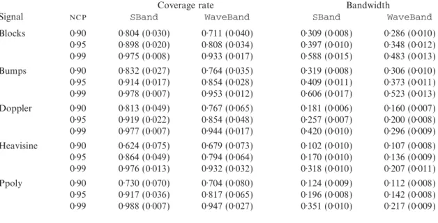
Table 1 gives simulation results. For each test function, computational problems occurred for between 2 and 33 signals while using WaveThresh. Results for WaveBand are based on signals that did not generate errors.
The SBand intervals have higher empirical coverage rates in every case but one, although they remain below the nominal coverage probabilities. Average widths of SBand intervals are greater
Fig. 1. Examples of SBand 95% pointwise credible intervals, with the original signal. Dots indicate data at n=1024 equally spaced points with addition of independent normally distributed noise with
502
C. S, A. C. D D. V. H
Table 1. Simulation results comparing mean coverage rates and widths for SBand and WaveBand credible intervals for nominal coverage probabilities () 0·90, 0·95 and 0·99. Standard errors are in brackets. T he five test functions were evaluated on n=1024 equally spaced points and rescaled to have standard deviation 1, and 1000 replications of noisy signals were created by adding independent normally distributed noise with r=4. Both methods used Daubechies’ least asymmetric wavelet with
eight vanishing moments, and default hyperparametersa=0·5 and b=1
Coverage rate Bandwidth
Signal SBand WaveBand SBand WaveBand
Blocks 0·90 0·804 (0·030) 0·711 (0·040) 0·309 (0·008) 0·286 (0·010) 0·95 0·898 (0·020) 0·808 (0·034) 0·397 (0·010) 0·348 (0·012) 0·99 0·975 (0·008) 0·933 (0·017) 0·588 (0·015) 0·483 (0·013) Bumps 0·90 0·832 (0·027) 0·764 (0·035) 0·319 (0·008) 0·306 (0·010) 0·95 0·914 (0·017) 0·854 (0·028) 0·409 (0·011) 0·373 (0·011) 0·99 0·978 (0·007) 0·953 (0·012) 0·606 (0·017) 0·523 (0·013) Doppler 0·90 0·813 (0·049) 0·767 (0·065) 0·181 (0·006) 0·160 (0·007) 0·95 0·919 (0·022) 0·854 (0·048) 0·257 (0·007) 0·200 (0·008) 0·99 0·977 (0·007) 0·944 (0·017) 0·420 (0·010) 0·296 (0·009) Heavisine 0·90 0·624 (0·075) 0·679 (0·073) 0·102 (0·010) 0·107 (0·008) 0·95 0·864 (0·049) 0·794 (0·064) 0·170 (0·010) 0·136 (0·009) 0·99 0·976 (0·013) 0·932 (0·032) 0·318 (0·010) 0·207 (0·011) Ppoly 0·90 0·730 (0·070) 0·704 (0·080) 0·124 (0·009) 0·112 (0·008) 0·95 0·917 (0·036) 0·817 (0·065) 0·196 (0·008) 0·142 (0·008) 0·99 0·988 (0·007) 0·947 (0·027) 0·351 (0·010) 0·217 (0·009)
than those of WaveBand. The coverage of SBand approaches the nominal coverage rate as this increases, perhaps because saddlepoint approximation can be highly accurate in the tails of a distribution.
Figure 2 compares the empirical coverage rates of SBand and WaveBand intervals at each t i for nominal coverage rates 95%. Coverage varies greatly across each signal, and is much better where the signal is smoother and less variable. This can be seen clearly in the results for the Blocks and Bumps functions, which have excellent coverages for the long constant parts. The coverage rates are also excellent for the low frequency portion of the Doppler function, but become less satisfactory when the frequency increases.
5. D
The SBand procedure uses the same prior distribution (3) as WaveBand, which depends critically on the parametersa and b. These parameters should in principle be chosen using prior knowledge about regularity properties of the unknown function. The case b=0 corresponds to prior belief that all coefficients on all levels have the same probability of being nonzero. This characterises self-similar processes such as white noise or Brownian motion. The case b=1 assumes that the expected number of nonzero wavelet coefficients is the same for each level. This is typical for piecewise polynomial functions, for example. The parametera is linked to the overall regularity of the signal. Large values ofa presuppose that the variablity of the wavelet coefficients around zero decreases quickly from one level to a higher frequency one, and thus that lower levels are sufficient to capture most of the signal’s features. We used the values a=0·5 and b=1 suggested by Abramovich et al. (1998) because they showed that these are robust choices in the absence of prior knowledge about the signal. However, other choices might lead to more efficient probability
Fig. 2. Empirial coverage rates () for SBand (lines) and WaveBand (dots) intervals for nominal coverage 95%. The five test functions were evaluated at n=1024 equally spaced points, and 1000 datasets withr=4 were used. Some signals were not taken into account
for WaveBand because results were unavailable.
intervals for some signals. Consider the Heavisine and Ppoly functions, which are the least irregular functions used for our simulations. The choice b=1 seems appropriate because Heavisine is a piecewise sine function, and Ppoly is a piecewise polynomial function. A larger value of a might be better, however, so Fig. 3 shows the mean empirical coverage rates of SBand for values of a between 0·2 and 10 and b=1. The intervals with nominal coverage probabilities 0·90, 0·95 and
504
C. S, A. C. D D. V. H
Fig. 3. Empirical coverage rates () for SBand intervals for values of a between 0·2 and 10, and b=1. The intervals with nominal coverage probabilities 0·90 (dotted), 0·95 (dashed) and 0·99 (solid) were computed on 200 noisy (a) Heavisine and ( b) Ppoly signals with n=1024 equally spaced points and r=4. The vertical
lines show the suggested default value, ata=0·5.
0·99 were computed on 200 Heavisine and Ppoly noisy signals with n=1024 equally spaced points and r=4. Coverage rates for the robust choice a=0·5 are poor compared to those with a=2. Thus careful choice ofa and b can improve coverage levels.
A
This work was supported by the Swiss National Science Foundation, and was performed while C. Semadeni was visiting the Department of Statistics and Applied Probability at the University of California, Santa Barbara, which he thanks for its hospitality.
R
A, F. & B, Y. (1995). Thresholding of wavelet coefficients as a multiple hypothesis testing procedure. In Wavelets and Statistics, Vol. 103 of L ecture Notes in Statistics, Ed. A. Antoniadis and G. Oppenheim, pp. 5–14. New York: Springer.
A, F., S, T. & S, B. W. (1998). Wavelet thresholding via a Bayesian approach. J. R. Statist. Soc. B 60, 725–49.
B, S., N, G. P. & S, B. W. (2002). Posterior probability intervals for wavelet thresholding. J. R. Statist. Soc. B 64, 189–205.
B, D. R. (1996). Uses of cumulants in wavelet analysis. J. Nonparam. Statist. 6, 93–114.
B, A. G. & G, H.-Y. (1996). Understanding WaveShrink: Variance and bias estimation. Biometrika 83, 727–45.
C, H. A., K, E. D. & MC, R. E. (1997). Adaptive Bayesian wavelet shrinkage. J. Am. Statist. Assoc. 92, 1413–21.
C, C. (1992). An Introduction to Wavelets. San Diego, CA: Academic Press.
D, H. E. (1954). Saddlepoint approximations in statistics. Ann. Math. Statist. 25, 631–50. D, H. E. (1987). Tail probability approximations. Int. Statist. Rev. 54, 37–48.
D, I. (1992). T en L ectures on Wavelets. Philadelphia, PA: SIAM.
D, A. C. (2003). Statistical Models. Cambridge: Cambridge University Press.
D, D. L. & J, I. M. (1994). Ideal spatial adaptation by wavelet shrinkage. Biometrika 81, 425–55.
D, D. L. & J, I. M. (1995). Adapting to unknown smoothness via wavelet shrinkage. J. Am. Statist. Assoc. 90, 1200–24.
H, C. C. & D, D. G. T. (1999). Bayesian wavelet analysis with a model complexity prior. In Bayesian Statistics 6, Ed. J. M. Bernardo, J. O. Berger, A. P. Dawid and A. F. M. Smith, pp. 769–76. Oxford: Clarendon Press.
J, J. L. (1995). Saddlepoint Approximations. Oxford: Clarendon Press.
M, S. G. (1989). A theory for multiresolution signal decomposition: The wavelet representation. IEEE T rans. Pat. Anal. Mach. Intel. 11, 674–93.
N, G. P. & S, B. W. (1994). The discrete wavelet transform in S. J. Comp. Graph. Statist. 3, 162–91.
P, D. & T, K. (2000). Adaptive confidence interval for pointwise curve estimation. Ann. Statist. 28, 298–335.
R, N. (1988). Saddlepoint methods and statistical inference (with Discussion). Statist. Sci. 3, 213–38. V, B. (1998). Nonlinear wavelet shrinkage with Bayes rules and Bayes factors. J. Am. Statist. Assoc.
93, 173–9.