HAL Id: halshs-00755682
https://halshs.archives-ouvertes.fr/halshs-00755682
Submitted on 21 Nov 2012HAL is a multi-disciplinary open access
archive for the deposit and dissemination of sci-entific research documents, whether they are pub-lished or not. The documents may come from
L’archive ouverte pluridisciplinaire HAL, est destinée au dépôt et à la diffusion de documents scientifiques de niveau recherche, publiés ou non, émanant des établissements d’enseignement et de
Mortality Convergence Across High-Income Countries :
An Econometric Approach
Hippolyte d’Albis, Loesse Jacques Esso, Héctor Pifarré I Arolas
To cite this version:
Hippolyte d’Albis, Loesse Jacques Esso, Héctor Pifarré I Arolas. Mortality Convergence Across High-Income Countries : An Econometric Approach. 2012. �halshs-00755682�
Documents de Travail du
Centre d’Economie de la Sorbonne
Mortality Convergence Across High-Income Countries : An Econometric Approach
Hippolyte d’ALBIS,Loesse Jacques ESSO,
Héctor
PIFARRÉi AROLASMortality Convergence Across High-Income
Countries: An Econometric Approach
∗
Hippolyte d’Albis
Paris School of Economics, University Paris 1
Loesse Jacques Esso
ENSEA (Abidjan)
Héctor Pifarré i Arolas
Toulouse School of Economics (LERNA)
October 13, 2012
Abstract
This work is devoted to the study of the variations of mortality pat-terns across a sample of high-income countries since 1960. We study changes in age-at-death distributions through two main indicators, life expectancy and Gini coefficient. We contribute to the ongoing debate over the existence of convergence amongst industrial countries in adult mortality by offering two main empirical regularities. First, we apply econometric tools commonly used in the economic growth literature to assess the existence of convergence across the countries in our sample; our results show that the convergence hypothesis is rejected when we consider the entire sample of industrialized countries. Second, we provide preliminary evidence of convergence among a subset of coun-tries. In this way, we offer empirics that justify further exploration into the theoretical underpinnings of subgroup convergence while present-ing evidence against convergence of all industrialized countries.
∗We thank Ronald Lee and Shripad Tuljapurkar for stimulating comments and the
1
Introduction
This work is devoted to the study of the variations of mortality patterns across high-income countries beginning in the 1960’s. We explore the ques-tion of whether age-at-death distribuques-tions have become more similar across this particular subsample of countries—that is, if there has been a process of convergence. We study distributions through their mean, i.e. the life expect-ancy, and their dispersion, measured with the Gini coefficient. According to this concept, we study convergence by observing the evolution of the disper-sion of the distributions for the two indicators in our sample of high-income countries.
Convergence is identified if the distribution across countries of a given indicator has become less unequal across time. We apply existing tools de-veloped in economic growth literature to study mortality convergence (see Durlauf et al. 2005, for a review of the literature). Using two ideas of con-vergence developed for economic growth, we can explore various aspects of the convergence process. First, we measure the extent to which gains in both mortality inequality reduction and life expectancy depend on initial levels of both in each country—that is, whether countries with lower starting life expectancy (or higher Gini index) have grown (or reduced) their indicators at a greater rate. This mode of convergence is denoted beta-convergence. Second, we observe the evolution of dissimilarities across countries. Our analysis directly contributes to the discussion on whether there is a greater dispersion of life expectations and mortality inequality across countries. This idea is captured in the concept of sigma-convergence or distributional
con-vergence. Additionally, we explore how these modes of convergence have behaved differently for particular periods since the 1960’s. Furthermore, a major contribution of this paper is the consideration of convergence without the necessity of approaching the same mortality distribution among all coun-tries. We propose the idea that there exist subgroups of countries that may converge to different mortality distributions and constitute what is known in economic growth literature as convergence clubs. We denote this difference as conditional convergence versus unconditional convergence.
We derive three main results from our econometric analysis. The first is on the catching-up process of adult mortality among developed countries for the period of 1960-2009. We show that there are greater improvements in the life expectancies of countries with lower life-expectancies while the over-all dispersion among high-income countries has not decreased. The second is on the reduction of mortality inequality. Countries starting with larger Gini coefficients have also experienced greater reductions in their coefficients. Des-pite that, however, it is also the case that dissimilarities in Gini coefficients across countries have not been reduced over time. Based on our evidence we conclude that according to our idea of convergence there is no reduction in the difference in mortality patterns between high-income countries. While we do not find evidence of convergence in the whole sample, our third result is preliminary evidence on the existence of sigma convergence among certain groups of countries or clubs. We implement a simple methodology to de-tect existing clubs and test the hypothesis of this type of convergence; our findings indicate the existence of such a phenomenon in the period of 1960-2009, although we do find evidence against conditional convergence in both
indicators in some subperiods.
Our paper is a contribution to the literature on convergence in mortal-ity patterns between countries. The topic has indeed been explored by a number of papers. Wilson (2001) suggests that there has been a process of demographic convergence from the 1950’s that involves both mortality and fertility. The author studies the world distribution of life expectancy and finds a decrease in its dispersion. This trend is nevertheless not observed for life expectancy at older age in high income countries (Glei et al. 2010). Other contributions have focused on convergence in inequality. For instance, Peltz-man (2009) shows that the inequality within countries, as measured by the Gini coefficient, decreases for a sample of countries. Edwards (2011) focuses on the length of life of a large sample of countries. By comparing a number of statistics for two given years (1970 and 2000) , he establishes that there is convergence in length of life at birth but not in adult mortality, specially among developed countries. In addition, he decomposes the total variance of the indicators in two sources: within and across countries. His findings indic-ate that even though the within variation has reduced, the across countries variation has remained broadly constant. A number of papers have studied the evolution of mortality patterns. In particular, Clark (2011) corroborates Peltzman (2009) findings but points out, in addition, that life expectancy improvements have been greater for developing countries while infant mor-tality reductions are larger in high-income countries. Eggleston and Fuchs (2012) study life expectancy in industrialized countries and point out that most gains in life expectancy have occurred in adult mortality, particularly concentrated after age 65. Finally, Bergh et al. (2010) study the effect of
globalization on life expectancy and find that even controlling for a number of other explanatory variables, the index of globalization of a country is pos-itively related to better life expectancies. These works have focused on one particular moment of the distribution and commented on its trends, leaving room for a formal more thorough analysis of the whole mortality distribution. This is addressed, in the contribution most closely related to our paper, by Edwards and Tuljapurkar (2005). Their work exploits the properties of the mortality distribution in order to assess whether there is convergence across countries and decomposes it in terms of convergence in mean and variance.
Earlier works in the topic often assess convergence considering life ex-pectancy. Our approach differs from these works in two main aspects. First, we study both the evolution of life expectancy and the dispersion of the dis-tribution for different countries and identify whether they converge in this additional dimension. This approach has been used in works like Edwards and Tuljapurkar (2005). A novelty in our work is the usage of the Gini index instead of the variance (or the standard deviation) as a measure of dispersion. This measure has been extensively used recently in the demography literat-ure dealing with mortality inequalities (for a discussion of its advantages, see Shkolnikov et al., 2003). Many other measures have been used to measure longevity dispersion, a survey is provided in Robine (2001). The use of the Gini coefficient can be justified by the fact that age-at-death distributions, even when truncated at age 10 or older, are not normally distributed. Ac-cording to the Gini coefficient, inequalities within countries have decreased for all the high-income countries of our sample. However, by using the stand-ard deviation of age-at-death distributions, Edwstand-ards and Tuljapurkar (2005)
conclude that inequalities have remained broadly constant.Second and most importantly, our methodology is also radically different from that of Edwards and Tuljapurkar’s (2005) because while they consider convergence as the shrinking of the distance to an ideal mortality distribution (that of Sweden 2002), we directly assess how the whole distributions of Gini coefficients and life expectancies across all countries considered have evolved. In Edwards and Tuljapurkar’s (2005) in order to have convergence it suffices that all individual countries improve their life expectancies and reduce their Ginis.
The paper is organized as follows. We first present our data set and discuss the indicators chosen for our analysis. We proceed in section 3 by formally analyzing the impact of initial conditions on the historical growth rate of our indicators. In the last two sections we analyze whether distri-butional convergence can be established. Concluding remarks are in section 6.
2
Indicators and descriptive statistics
Our object of study, mortality patterns, is extracted from the period life-tables available in Human Mortality Database. The scope of our analysis is narrowed to a group of high-income countries (see list in Appendix 7.1). We consider, but do not restrict to, the whole life-table. We also study adult mortality, as measured by deaths of age 10 or more, and female mortality. Following Edwards and Tuljapurkar (2005), we hence may discuss the par-ticular effects of changes in infant mortality and isolate the sex differences in mortality evolution. Although this section of the paper focuses on the mortality distribution of the female population over 10 at time of death,
the descriptive statistics for other distributions, including distributions with infant mortality, can be found in Appendix 7.3.
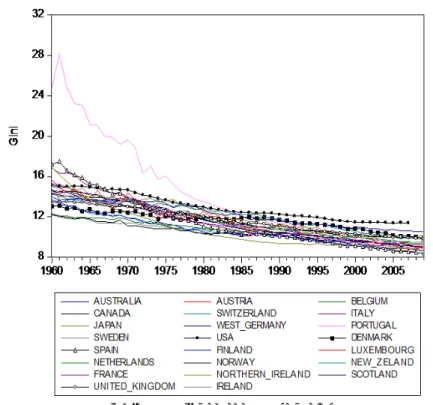
The first indicator we consider is the life expectancy. Figure 1 presents the series of female’s life expectancies at age 10 between 1960 and 2009 for the countries in our sample.
Figure 1. Life expectancy at age 10, females.
A first look at the evolution of life expectancies reveals a common trend in all the countries in the sample: they have increased steadily in all countries and there does not appear to be an obvious slowdown in the amelioration of life spans. This pattern is also observed among the other distributions we consider (see Figures 7, 8 and 9 in Appendix 7.3). Further scrutiny reveals that the speed of amelioration has not been the same for all countries. In the time span considered, new differences across countries are created by the variety of growth rates. For instance, life expectancy in Japan has evolved from the last to the first position.
In our analysis we recognize the importance of studying the life-tables dynamics beyond life expectancy changes by focusing on an important and additional piece of information of the distribution, its dispersion that meas-ures inequality in longevity. Given the non normality of the distribution, which we formally test in Appendix 7.2, we rely on a scale independent measure of inequality. We propose to compute a Gini coefficient to capture the dispersion of the distribution. The Gini coefficient consists in a compar-ison of the cummulative distribution of years by fraction of the population of the actual distribution and the cummulative of an hypothetical egalitarian distribution in which every member of the society lives for the same number of years. As usual, a Gini coefficient equal to zero indicates perfect equality, that is, all individuals have died at the same age; the closer to one, the less egalitarian a distribution is. A number of different formulations have been proposed for the study of life tables (see Shkolnikov et al., 2003). Most not-ably, it is possible to rephrase the concept in terms of differences between individual ages at death. We follow this approach and, since we may trun-cate our distributions at age 10 to eliminate child mortality, we present the following formula to compute the Gini coefficient at any age :
= P P () ()|() + ()− ()− ()| 2 ()2
where is the life expectancy at exact age , is the number of survivors
at exact age (with 0 = 100 000), is the number of deaths between ages
and + 1, and the is the average length of survival between ages and
+ 1 for persons dying in the interval.
series of Gini coefficients computed for female’s truncated distributions.
Figure 2. Gini at age 10, females.
The evolution pattern of the Gini coefficients is much less clear than that of the life expectancy. In both the case of the female-only distribution and the case of both genders (Figure 12 in Appendix 7.3) there is a common trend of the reduction of mortality inequalities. However, some countries have shown increasing inequalities over the early years of the sample, such as the case of the United States, or more notably, Denmark. As expected, the decrease in Gini coefficients is more pronounced if child mortality is included (see Figures 10 and 11 in Appendix 7.3).
3
Convergence and initial conditions
A first way of assessing convergence across countries hinges on a negative relationship between the growth rate of a variable and its initial value. In
economic growth empirics, the econometric analysis of such a relationship is named a beta-convergence analysis.
Formally, let be a variable (i.e. the logarithm of the life expectancy or the Gini coefficient) and be an observation of for country at date
= 0 1 . Early statistical analyses of convergence have focused on the properties of coefficient in regressions of the following equation:
= + 0+ (1)
where = 1 ( − 0) is the average growth rate of the variable at stake
between the initial and terminal dates. The idea is to study whether countries with lower, for life expectancy, (or higher, in the case of the Gini index) values have experienced larger increases (or, respectively, decreases). The confirmation of the hypothesis of beta-convergence corresponds to a negative estimate for the linear regression coefficient in equation (1).
We display our results of for estimations vis à vis life expectancy in Table 1. This table reports the results for regressions based on equation (1) for the five periods we consider. They indicate that beta-convergence has taken place in the period 1960-2009; countries with lower initial life expectancies have experienced the largest increases in life expectancies. However, it is interesting to note that the process has not been the same for the entire time span and that for certain periods it depends on whether the distribution is truncated. For the whole distribution, the initial condition is significantly negative up until 1980, followed by a period of no beta-convergence in 1990-2009. Thus most of the catching-up process occurred up to 1980, while
further convergence afterwards occurred only for the sample as a whole. 1960-2009 1970-2009 1980-2009 1990-2009 2000-2009 ˆ 0 −0019∗ (−6775) −0018 ∗ (−4822) −0012 ∗ (−2793) −0005(−1165) −0012 ∗∗ (−1897) ˆ 10 −0018∗ (−4130) −0016 ∗ (−3121) −0009 ∗∗ (−1890) −0003(−0833) −0010(−1684) ˆ 0 −0021∗ (−6124) −0020 ∗ (−4172) −0014 ∗ (−2380) −0004(−0686) −0010(−0676) ˆ 10 −0021∗ (−3588) −0017 ∗ (−2417) −0010(−1575) −0002(−0314) −0009(−1567)
Notes: the ˆ denote OLS estimates for in eq. (1) for the whole ( = 0) and truncated ( = 10)distributions of both genders ( = )and females only ( = ) populations. t-statistics are in (.). * denotes significance at 5%.
Table 1. beta-convergence in life expectancy
The results of the beta-convergence analysis applied to the Gini coefficient are presented in Table 2. As before, we estimate equation (1) for the same periods. For all distributions we consider, the initial value significantly affects the (negative) growth rate until the period 1980-2009, when the catching-up process between higher and lower inequality countries ceased.
1960-2009 1970-2009 1980-2009 1990-2009 2000-2009 ˆ 0 −0020∗ (−17118) −0023 ∗ (−11191) −0022 ∗ (−4950) −0026 ∗ (−2796) −0016(−0965) ˆ 10 −0020∗ (−21932) −0024 ∗ (−13834) −0023 ∗ (−5752) −0027 ∗ (−2997) −0019(−1169) ˆ 0 −0021∗ (−18357) −0025 ∗ (−11367) −0022 ∗ (−4906) −0020 ∗ (−2482) −0002(−0177) ˆ 10 −0021∗ (−22347) −0025 ∗ (−13423) −0023 ∗ (−5440) −0017 ∗ (−2268) −0004(−0557)
Notes: the ˆ denote OLS estimates for in eq. (1) for the whole ( = 0) and
truncated ( = 10)distributions of both genders ( = )and females only ( = ) populations. t-statistics are in (.). * denotes significance at 5%.
Table 2. beta-convergence in Gini coefficients
While beta-convergence is informative and necessary for convergence, it is by no means a sufficient condition. In the short-run, a larger growth rate does not imply catching up. The difference in starting values could result in lower absolute values of amelioration for that period of time. Furthermore,
countries may experience non monotonic dynamics or may converge to differ-ent steady-states. Given these limitations, we turn to the more demanding concept of distributional convergence.
4
Distributional convergence
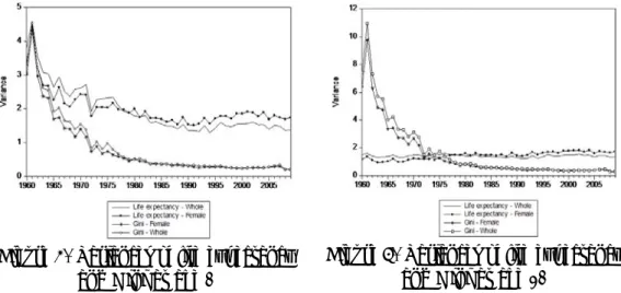
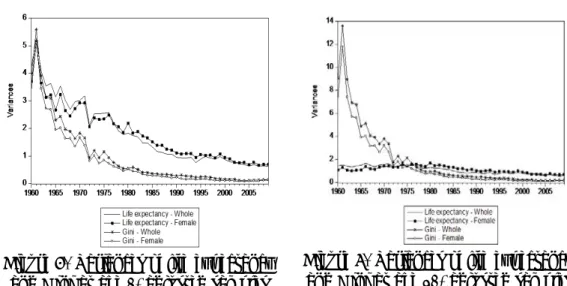
In this section we focus on the dynamics of the shape of the cross-countries distributions of our mortality indicators, i.e. life expectancy and Gini coeffi-cient at ages 0 and 10. Figures 3 and 4 plot the variance1 of these distribu-tions.
Figure 3. Variances of life expectancy and Gini at age 0
Figure 4. Variances of life expectancy and Gini at age 10
The evolution of the variances provides an illuminating hint: there are no appreciable differences between the late 1970’s and the end of the period and, upon existence, the decrease takes place over the period 1960-1975. But for truncated distributions (Figure 4), the variance of life expectancies of female population is even higher nowdays than in 1960. This already suggests preliminary evidence against a process of convergence and, as formalized below, we show this graphical intuition to be true.
1One could have also computed a variance weighted by the relative size of the countries
Distributional convergence, also named sigma-convergence, is formally studied as follows. Let be a variable (logarithm of life expectancy or Gini coefficient) and be an observation of for country at date . Let 2()
be the variance of across countries at date The distribution of has converged between time and + if and only if 2
()− 2+() 0.
A traditional statistical test for convergence of variable is the test of the null hypothesis of no convergence, i.e. testing whether 2() = 2+().
To do so, a number of authors (see Durlauf et al., 2005, for a review of the literature) have proposed the following regression specification:
= + + + (2)
where is the mean growth rate of variable between and + for country
, and where the slope of the relationship is defined as: = 1 µ 1− ( +) 2 +() 
If the estimate for is significant and negative, this means, using the Cauchy-Schwartz inequality, that the standard deviation has decreased over time, i.e.
() +()
Conversely, if the estimate of is non-negative, nothing about convergence can be deduced from equation (2). Even if ˆis positive and significant, there is not enough evidence to tell anything about convergence. It does not mean there is divergence.
Our test for sigma-convergence (Table 3) establishes the fact that the dis-similarities across high-income countries in life expectancy have not shrunk.
The distribution of the life expectancies at age 10 of high-income countries stands as unequal as it was in the beginning of the period. Furthermore, this result is robust to gender differences, the inclusion of infant mortality and holds for most of the subperiods considered. It confirms, if needed, that beta-convergence does not guarantee a trajectory towards a less disperse cross section. For an intuition of this result, recall the particular case of Japan, a country which started from last place in life expectancy and ended in the top position. Although this is only an example, it illustrates the possibility that the catching-up process is not related to the reduction of the differences.
1960-2009 1970-2009 1980-2009 1990-2009 2000-2009 ˆ 0 0015 (1675) 0010(1204) 0002(0354) 0002(0370) −0005(−0665) ˆ 10 0017∗ (3098) 0014 ∗ (2287) 0005(0913) 0002(0557) −0004(−0598) ˆ 0 0021∗ (2972) 0017 ∗ (2345) 0010(1394) 0006(1253) −0004(−0575) ˆ 10 0021∗ (4914) 0019 ∗ (3684) 0011 ∗∗ (1879) 0007(1461) −0003(−0552)
Notes: the ˆdenote OLS estimate for in eq. (2) for the whole ( = 0) and
truncated ( = 10)distributions of both genders ( = )and females only ( = ) populations. t-statistics are in (.). * and ** denotes significance at 5% and 10%.
Table 3. sigma-onvergence in life expectancy
Our results regarding sigma-convergence in Gini coefficients (Table 4) are also supportive of a non-convergence hypothesis overall. If we consider the entire (both genders) distribution of adult mortality, we can only reject the hypothesis of convergence for the most recent subperiods. In the remaining subperiods, the coefficient is positive but not significantly so. For the females-only distribution, we obtain significantly positive for the entire time span as well as the last subperiod. Still, it is worth noting that in no case does the hypothesis of convergence hold. Furthermore, if we restrict ourselves to considering female mortality, for the whole period 1960-2009, we
reject with significance the hypothesis of convergence. 1960-2009 1970-2009 1980-2009 1990-2009 2000-2009 ˆ 0 0006 (0274) 0006(0362) 0004(0412) 0021 ∗∗ (1816) 0028 ∗∗ (1889) ˆ 10 0003 (0126) 0003(0137) 0001(0101) 0018(1456) 0024(1561) ˆ 0 0037∗∗ (1873) 0023(1313) 0005(0481) 0012(1185) 0018 ∗∗ (1781) ˆ 10 0042 (1682) 0024(1158) 0004(0332) 0009(0934) 0016(1474)
Notes: the ˆdenote OLS estimate for in eq. (2) for the whole ( = 0) and
truncated ( = 10)distributions of both genders ( = )and females only ( = ) populations. t-statistics are in (.). * and ** denotes significance at 5% and 10%.
Table 4. sigma-convergence in Gini coefficients
We conclude that for both indicators, life expectancy and mortality inequal-ity, the cross section of high-income countries stands as disperse in 2009 as in 1960. We have formally tested this hypothesis with the sigma-convergence regression and according to this idea of convergence, there has not been a reduction of differences among the adult mortality patterns of developed countries. Our results regarding beta-convergence show that the relative po-sitions of countries in the sample, however, have been altered, indicating that there have indeed been relevant changes, but not with regards to convergence. Although our findings rely on the definition of convergence, we believe that convergence is best assessed by the study of the moments of the cross sec-tion of countries. Even should a common steady state across countries exist (whereby countries necessarily approach a single life table distribution), in the meanwhile and for a particular period of history, convergence still should be assessed by how countries compare relative to one another. By doing so, one avoids the fundamental problem of identifying the steady state, as our measure of convergence is independent of it. In the next section we carry the analysis one step further and suggest that the presumption that there exists
a unique steady state must be formally tested.
5
Conditional distributional convergence
In the previous section we implicitly assumed that mortality indicators of all countries were to converge to the same value, denoted as a steady state. In a different form, as emphasized in the introduction, this is the underly-ing hypothesis for earlier work (Edwards and Tuljapurkar, 2005). We now study conditional convergence, where groups of countries converge to dif-ferent steady states (this hypothesis has also been discussed in Lee, 2006). Our discussion focuses on life expectancy and Gini coefficients, as this choice reflects our interests in obtaining measures independent of the scale of meas-urement and reflective of relative distances between countries.
We want to explore the hypothesis of the existence of structural differences among countries that have manifested in a permanent influence on groups of countries, leading to different steady states. Possible examples of par-ticular factors might include climatic conditions, dietary or smoking habits and national health systems (for further discussion, see Preston, 1980). In this paper, we propose a preliminary exploration of this hypothesis. A more rigorous analysis would require evidence of the relevant conditions for the determination of the different steady states.
The following algorithm is used for determining clubs: we begin with = 1 countries each of which we follow with a given indicator—the life expectancy or the Gini coefficient—over time and find no convergence. Seeing no convergence amongst N countries, we systematically remove a single country from the group and compute the difference between the initial
and final variances of the indicator for each possible N-1 set (N sets in total). We then select the set that shows the greatest decrease in variances and see if sigma-convergence occurs in this set. If not, we continue the removal process and systematically remove a single country from the N-1 set and compute the difference between the initial and final variances of the indicator for each possible N-2 set (N-1 sets in total). We again test for sigma-convergence. We iterate until we find a subset of countries for which there is sigma-convergence or until the sample is reduced to a number of countries where results would no longer be statistically satisfactory. Finally, we repeat the algorithm for the distribution of both sexes and that of only females. As a robustness check, we perform the algorithm for the distributions including child mortality.
The following are the results for testing only for sigma-convergence in our adjusted samples. The reason is that since beta-convergence is observed for the whole sample, it will necessarily be observed for the adjusted ones. Moreover, we ultimately judge the existence of convergence on the results of the sigma-convergence tests. We have different adjusted samples for every indicator and distribution; a list of them is provided in the Appendix.
Graphically, the evolutions of the variances of both indicators, as charac-terized in Figures 5 and 6, differ greatly from those presented in Figures 3 and 4, since a decrease is now observed even when child mortality is excluded. We observe a sharp decrease in the variance of the life expectancy, which is
especially pronounced in the earlier part of the time span (1960-1970).
Figure 5. Variances of life expectancy and Gini at age 0, adjusted samples
Figure 6. Variances of life expectancy and Gini at age 10, adjusted samples
The results of our estimation (Table 5) reveal that there has been con-vergence in life expectancy (both at birth and at age 10) for the mortality distributions including both genders. In particular, for the whole sample, convergence occurs in the entire time span and the middle periods 1970-2009 to 1990-2009 but not for the last period 1960-2009. In the case of the entire adult population, convergence only occurs in the last periods, 1980-2009 and onwards. Interestingly, we do not find support for the hypothesis of conver-gence for the female-only distribution for the period 1960-2009. There is, however, evidence of convergence for the restricted female samples for the
period 1980-2009. 1960-2009 1970-2009 1980-2009 1990-2009 2000-2009 ˆ 0 −0003∗∗ (−1872) −0013 ∗ (−2214) −0013 ∗ (−2395) −0004 ∗ (−2485) −0008(−0543) ˆ 10 0005 (0650) 0001(0167) −0005 ∗∗ (−1535) −0003 ∗∗ (−1450) −0009 ∗∗ (−1728) ˆ 0 0010 (0880) 0005(0431) −0006 ∗∗ (−1581) −00005(−0051) −0005(−0388) ˆ 10 0012∗ (2060) 0008(1038) −0004 ∗∗ (−1384) −00007(−0077) −0005(−0394)
Notes: the ˆdenote OLS estimate for in eq. (2) for the whole ( = 0) and
truncated ( = 10)distributions of both genders ( = )and females only ( = ) populations. t-statistics are in (.). * and ** denotes significance at 5% and 10%.
Table 5. sigma-convergence in life expectancy, adjusted samples
To better understand this result, we test for convergence in male-only mor-tality (see Table 6) and find that there is convergence for both samples (adult males and whole sample) when considering the entire time span. This result is weakened for the male adults sample, since the later subperiods do not show statistically significant evidence of convergence (1980-2009 onwards). Given this evidence, we conclude that the observed convergence is not likely to be driven by a reduction in the differences across sexes.
1960-2009 1970-2009 1980-2009 1990-2009 2000-2009 ˆ 0 −0016∗∗ (−1584) −0019 ∗ (−2343) −0011 ∗∗ (−1522) −0005 ∗∗ (−1818) −0005(−0410) ˆ 10 −0003∗∗ (−1410) −0001 ∗ (−2168) −00007(−0001) −0004(−0696) −0006(−0554)
Notes: ˆ0and ˆ10denote OLS estimate for in eq. (2)
for whole and truncated distribution of male populations. * denotes significance at 5%.
Table 6. sigma-convergence in Life expectancy, adjusted samples
We find conclusive results regarding the Gini index (Table 7) in favor of the conditional convergence hypothesis. When we consider the entire period, convergence is robust to the inclusion of child mortality. It is noteworthy that convergence occurred in the first part of the time span (until the period
1990-2009, not included), especially for future work unpacking the causal explanations behind convergence from an historical standpoint among others. Restricting our sample to female mortality has similar results as that of life expectancy. 1960-2009 1970-2009 1980-2009 1990-2009 2000-2009 ˆ 0 −0006∗∗ (−1635) −0006 ∗∗ (−1791) −0007 ∗∗ (−1599) 0014 (0961) 0027 ∗∗ (1481) ˆ 10 −0010∗ (−2321) −0011 ∗∗ (−1437) −0011 ∗∗ (−1843) 0011 (0696) 0025(1246) ˆ 0 0032∗∗ (1451) 0017(0755) −00008 ∗ (−2059) 0011(0867) 0029 ∗ (2323) ˆ 10 0036 (1153) 0017(0067) −0002 ∗ (−2158) 0008 (0615) 0027 ∗ (2035)
Notes: the ˆdenote OLS estimate for in eq. (2) for the whole ( = 0) and
truncated ( = 10)distributions of both genders ( = )and females only ( = ) populations. t-statistics are in (.). * and ** denotes significance at 5% and 10%.
Table 7. sigma-convergence in Gini coefficients, adjusted samples
6
Conclusion
In this work, we tested the hypothesis of convergence in adult mortality patterns in high-income countries for a period of 49 years. First, we evaluated convergence with the underlying idea that all countries are approaching a common steady state, or what is termed unconditional convergence. To do so, we proposed a concept of convergence based on observing whether the distribution of some given indicators have become less disperse over time. Our results empirically reject this hypothesis for both life-expectation and mortality inequality as measured by the Gini coefficient. Nevertheless, we also provided evidence that there have been changes in this period in the relative positions of countries in terms of both life expectancy and mortality inequality.
convergence clubs, formed by groups of countries that converge to a common steady state distribution of mortality. Our results support the hypothesis of conditional convergence in both the Gini coefficient and life expectancy; however, this mode of convergence does not hold for certain subperiods. Given there is convergence for the male-only sample, we conclude that this is likely not due to a reduction in the dissimilarities across genders.
There are many related issues which we do not address in this paper out of an understanding of both the scopes of the issues and the constraints of this paper. Some of these issues deserve further attention in next step pro-jects. For instance, we do not provide an account of the changes in mortality causes that have driven the changes observed in the mortality distributions, nor tried to relate them to the health policies adopted by the different coun-tries. A natural next step would be to investigate the causes of death that have evolved similarly for all countries and identify the ones creating the differences we still observe. For older ages, this has been recently studied by the National Research Council (2010). Furthermore, although we have introduced the idea of conditional convergence, we have studied it only up to the extent of illustrating the justification for further exploration. A rigorous analysis would require identifying the common traits relevant to mortality patterns among countries constituting a convergence club. Naturally, the possibility of more than one convergence club should also be considered.
Finally, one could question our choice of studying countries instead of individuals. Indeed, if the focus is on welfare (Edwards, 2012), it seems reas-onable to have individuals as unit of analysis (see Bourguignon and Chris-tian Morrisson, 2002, for a work that takes this approach and more recently
Becker et al., 2005). Studying the convergence patterns across countries, however, improves our understanding of crucial topics such as the existance of a common mortality distribution or what are the factors that contribute to the dynamics of mortality. Issues that are directly related to specific ap-plications such as the forecasting of mortality dynamics (see for instance Li and Lee, 2005) or the evaluation of national health policies.
7
Appendix
7.1
Samples of countries
Throughout the paper, we use a number of different samples. First, we have tested unconditional convergence on the following sample of high-income countries.
Whole sample: Australia, Austria, Belgium, Canada, Switzerland, Italy, Japan, West Germany, Portugal, Sweden, USA, Denmark, Spain, Finland, Luxembourg, Netherlands, Norway, New Zealand, France, Northern Ireland, Scotland, Britain, Ireland, Israel
Second, we have constructed a number of adjusted samples, obtained according to the method described in the text, to test for conditional con-vergence. For simplicity, we report the countries excluded from the whole sample.
Life expectancy at 0 in the whole population: USA, Denmark, Scot-land, Australia, Japan.
Life expectancy at 10 in the whole population: USA, Denmark, Scot-land, SwitzerScot-land, Japan
Life expectancy at 0 in the female population: USA, Denmark, Scot-land, Italy, Japan.
Life expectancy at 10 in the female population: USA, Denmark, Scot-land, Italy, Japan.
Gini of age-at-death at 0 in the whole population: USA, Scotland, Italy, Finland, United Kingdom
Gini of age-at-death at 10 in the whole population: USA, Scotland, Italy, United Kingdom, Finland
Gini of age-at-death at 0 in the female population: USA, Scotland, Italy, Spain, Denmark.
Gini of age-at-death at 10 in the female population: USA, Scotland, Italy, Spain, Denmark.
7.2
Testing the normality assumption
Cramer-von Mises, Anderson-Darling, and Watson nonparametric empirical distribution tests can be used to verify the normality for truncated ages-at-death distributions for Sweden and United States for the year 2000. These tests are based on the comparison between the empirical distribution and the theoretical normal distribution functions and use the estimates for the mean and standard deviation of the empirical distributions based on the data. For a general description of empirical distribution function testing, see d’Agostino and Stephens (1986). The results in Table 8 summarize the outcome of the
statistical tests.
Sweden United States
Parameter estimates Mean 90089 [7457] 90094[8683] Standard deviation 127290 [14832] 109316[14832] Log likelihood −95055 −93365
Empirical distribution test
Cramer-von Mises 236 (0000) (0000)178 Watson 211 (0000) (0000)160 Anderson-Darling 1280 (0000) 1014(0000)
Notes: Z-statistics are in [.]. Numbers in (.) are p-values.
Table 8. Non-parametric normality tests for the distributions of age-at-death.
Table 8 is composed of two parts. The first is on the estimates for paramet-ers (mean and standard deviation) that characterize a normal distribution, and the second presents the results of the normality tests. It is shown that for both distributions (Sweden and United States), the estimation of the mean and the standard deviation are statistically significant at the 1% level. When evaluated formally, the tests demonstrate that the hypothesis that the distributions of ages-at-death for Sweden and the United Sates, even when truncated below age 10, follow a normal distribution is rejected at the 1% significance level. This conclusion provides evidence that the Kullback-Leiber divergence approach seems inappropriate for studying distributional convergence in mortality.
7.3
Further descriptive statistics
In the core of the text, we presented the indicators computed with distribu-tions of the age-at-death truncated at age 10 for female. The indicators for
other distributions we consider are reproduced below.
Figure 7. Life expectancy at age 0, females.
Figure 10. Gini coefficient at age 0, females.
Figure 8. Life expectancy at age 0, both genders.
Figure 11. Gini coefficient at age 0, both genders.
Figure 9. Life expectancy at age 10, both genders.
Figure 12. Gini coefficient at age 10, both genders.
References
[1] Becker, Gary S., Tomas J. Philipson and Rodrigo R. Soares. 2005. “The quantity and quality of life and the evolution of world Inequal-ity,”American Economic Review 95(1): 277-291.
[2] Bergh, Andreas and Therese Nilsson. 2010. “Good for living? On the relationship between globalization and life expectancy,”World Develop-ment 38(9): 1191-1203.
[3] Bourguignon, François, and Christian Morrisson. 2002. “Inequality Among World Citizens: 1820-1992,”American Economic Review 92(4): 727-744.
[4] Clark, Rob. 2011. “World health inequality: Convergence, divergence, and development,”Social Science & Medicine 72(4): 617-624.
[5] D’Agostino, Ralph B. and Michael A. Stephens. 1986. Goodness-of-Fit Techniques, Marcel Dekker, Inc., New York.
[6] Durlauf, Steven N., Paul A. Johnson and Jonathan R.W. Temple. 2005. “Growth econometrics,”in Philippe Aghion and Steven Durlauf (eds.), Handbook of Economic Growth, Elsevier, pp. 555-677.
[7] Eggleston, Karen N., and Victor R. Fuchs. 2012. “The new Demo-graphic Transition: Most gains in life expectancy now realized late in life,”Journal of Economic Perspectives, 26(3): 137-56.
[8] Edwards, Ryan D. 2011. Changes in world inequality in length of life: 1970-2000," Population and Development Review 37(3): 499-528. [9] Edwards, Ryan D. 2012. “The cost of uncertain life span,” Journal of
Population Economics, forthcoming.
[10] Edwards, Ryan D. and Shripad Tuljapurkar. 2005. “Inequality in life spans and a new perspective on mortality convergence across industri-alized countries,”Population and Development Review 31(4): 645-674. [11] Glei, Dana A., France Meslé and Jacques Vallin. 2010. “Diverging trends
in life expectancy at age 50: A look at causes of death,” in Eileen M. Crimins, Samuel H. Preston and Barney Cohen (eds.), International Differences in Mortality at Older Ages: Dimensions and Sources. Wash-ington, DC: The National Academies Press.
[12] Human Mortality Database. 2012. University of California, Berkeley (USA), and Max Planck Institute for Demographic Research (Germany). Available at www.mortality.org.
[13] Li, Nan and Ronald Lee. 2005. “Coherent mortality forecasts for a group of populations: An extension of the Lee-Carter method,”Demography 42(3): 575-594.
[14] Lee, Ronald. 2006. “Mortality Forecasts and Linear Life Expectancy trends,”in Bengtsson, Tommy (ed.), Perspectives on Mortality Forecast-ing III. The Linear Rise in Life Expectancy: History and Prospects. So-cial Insurance Studies. No. 3., Stockholm: Försäkringskassan, Swedish Social Insurance Agency, pp. 19-39.
[15] National Research Council. 2010. International Differences in Mortality at Older Ages: Dimensions and Sources. Eileen M. Crimins, Samuel H. Preston and Barney Cohen (eds.), Washington, DC: The National Academies Press.
[16] Peltzman, Sam. 2009. “Mortality inequality,” Journal of Economic Per-spectives 23(4): 175-190.
[17] Preston, Samuel. 2010. “Causes and consequences of mortality declines in less developed countries during the twentieth century,”in Richard Easterlin (ed.), Population and Economic Change in Developping Coun-tries. Chicago: University of Chicago Press.
[18] Robine, Jean-Marie. 2001. “Redéfinir les phases de la transition épidémi-ologique à travers l’étude de la dispersion des durées de vie: le cas de la France,” Population (French Edition) 56(1): 199-221.
[19] Shkolnikov, Vladimir M., Evgeny E. Andreev and Alexander Z. Begun. 2003. “Gini coefficient as a life table function: Computation from dis-crete data, decomposition of differences and empirical examples,” Demo-graphic Research 8(11): 305-358.
[20] Whitehouse, Edward R. and Zaidi Asghar. 2008. “Socio-economic dif-ferences in mortality: Implications for pensions policy,”OECD Social, Employment and Migration Working Papers 71.
[21] Wilmoth, John R., Carl Boe and Magali Barbieri. 2010. “Geographic differences in life expectancy at age 50 in the United States compared with other high-income countries,” in Eileen M. Crimins, Samuel H. Preston and Barney Cohen (eds.), International Differences in Mortality at Older Ages: Dimensions and Sources. Washington, DC: The National Academies Press.
[22] Wilson, Chris. 2001. “On the scale of global demographic convergence 1950-2000,”Population and Development Review 27(1): 155-171.