HAL Id: halshs-00551485
https://halshs.archives-ouvertes.fr/halshs-00551485
Submitted on 3 Jan 2011HAL is a multi-disciplinary open access archive for the deposit and dissemination of sci-entific research documents, whether they are pub-lished or not. The documents may come from teaching and research institutions in France or abroad, or from public or private research centers.
L’archive ouverte pluridisciplinaire HAL, est destinée au dépôt et à la diffusion de documents scientifiques de niveau recherche, publiés ou non, émanant des établissements d’enseignement et de recherche français ou étrangers, des laboratoires publics ou privés.
Simulating urban networks through multiscalar
space-time dynamics (Europe and United States, 17th
-20th centuries)
Anne Bretagnolle, Denise Pumain
To cite this version:
Anne Bretagnolle, Denise Pumain. Simulating urban networks through multiscalar space-time dy-namics (Europe and United States, 17th -20th centuries). Urban Studies, SAGE Publications, 2010, 47 (13), pp.2819-2839. �halshs-00551485�
Simulating urban networks through multiscalar space-time dynamics (Europe and United States, 17th -20th centuries)
Bretagnolle A., Pumain D., last version before publication in Urban Studies, n° spécial « Urban Networks », vol. 47, n°13, November
Introduction
Urban systems are complex because of the multiple interdependencies, often non-linear, which interconnect the cities and alter their dynamic trajectory. These systems are characterised by emerging properties, which are mainly the product at a wide geographical scale of interaction processes operating at lower scales (Pumain, 2000). We have long observed self-organising processes in these systems, which are translated, on a global scale by quite regular types of hierarchies and urban networks, as well as by organising the functional specialities of the cities into networks (Bretagnolle et al., 1998 and 2000, Taylor et al., 2006, Cattan, 2007). The creation of models which simulate this growth has several aims. On the one hand, it involves checking that the theoretic processes identified as being responsible for the emergence of the urban system properties are effectively in the position to generate such properties, and possibly prioritise the importance of each of these processes. On the other hand, by comparing the simulations of urban system developments in the different geographic, economic, political and historic contexts, it should also be possible to more precisely measure the role of each of these contextual effects, beyond the general aspects of a generic growth summarised by stylised facts.
Among the large variety of urban dynamic models (Pumain, 1998), the multi-agent models are particularly well adapted to this formalisation and give meaning to a hypothetical-deductive process: they permit frequent coming and going between the theory injected into the rules and parameters of the model, the resulting simulations and the historical observations. This type of model was first applied in geography precisely to the simulation of settlement systems (Bura et al., 1996, Sanders et al., 1997). In the line of this first model, which has been substantially transformed, the Simpop2 model was created as a generic model, simulating the growth of a group of cities interacting under the hypotheses of competition, formalised by the spatial operating of an exchange market (Bretagnolle et al. 2006, Pumain et al. 2006b). These cities become heterogeneous through the diversity of their socio-economic functions and through their more or less successful incorporation into the exchange networks. Different specific models were built from the generic model, for example the Eurosim model (Sanders et al., 2007). The applications presented here are developed for a long evolution (3 to 7 centuries) and are interested in reproducing stylised facts rather than precisely located information. The modelling process is closely guided by a constant recourse to historical sources (city populations, economic activities, transport networks), thereby participating in data-driven simulation methods. We compare the urban system growth processes in early urbanised countries (illustrated by the case of Europe between 1300 and 2000) and those of new countries (the example chosen is the United States from 1650 to 2000). The simulations show strong similarities which confirm the solidity of the urban growth theory tested by the model, but also reveal fundamental differences in the way the cities use and occupy the geographical space. 1 Theoretical and empirical basis for modelling urban systems
In order to develop a model which simulates the evolution of urban systems, three important ingredients are needed: a sound theory about the main processes driving the evolution, a significant set of relevant stylised facts which summarise the main descriptive features of urban systems and their evolution, and some carefully designed historical data bases for calibrating the model. According to the current state of the art, a rather general agreement can be made about descriptive stylised facts, but we are still lacking a complete evolutionary theory for urban systems, and most data sources are not readily usable for long term historical studies.
1.1 Stylised facts: emerging properties at the level of cities networks
Urban systems and their evolution have been analysed in numerous empirical studies. Some are comprehensive, including quantitative aspects of urban size and growth as well as qualitative features of functional differentiation (for instance Christaller, 1933, Berry, 1964, Bourne et al., 1984, Pred, 1966, 1973 and 1977, Robson, 1973, Pumain, Saint-Julien, 1984, Black and Henderson, 2003 among others), others are restricted to the question of city size distribution (Zifp, 1941, for recent reviews see Nitsch, 2005 and Pumain, 2006). From these studies, there are without discussion a few generic properties which seem to characterize any urban system in the world: first, a very contrasted hierarchy of city sizes, which is generally represented by a highly skewed statistical distribution, of a lognormal type, and approached in its upper part by a Zipf or Pareto distribution; second, a series of urban socio-economic specialisation which can be divided between those whose presence is correlated with city size (as assumed in central place theory but also including innovative functions Pumain et al., 2006a), and more specialised activities which emerge in a few cities only.
The main challenges for building a comprehensive theory of urban systems arise when interpretations are given for linking these stylised facts. Roughly, most economists insist on the effect of agglomeration economies, or localised information and knowledge spillover, at the origin of urban hierarchy, as an intrinsic property of urban size (Gabaix, 1999) or as reflecting the choice of a port-folio of economic activities (Henderson, 1985, Fujita et al., 2001), whereas geographers and evolutionary economists try to link these effects with the competition and emulation between cities for innovation, involving a variety of networks that are transforming over time (Hall, 1998, Frenken and Boschma, 2007). In the first case, the theory is micro founded (Duranton, Puga, 2004) and most often defining the structure of urban systems as in equilibrium whereas in the second case, the consideration of multiple scales of time and space is required for an open evolutionary perspective.
Like other complex systems, the urban systems are characterised by a visible dichotomy between the behaviour of elementary entities, on a mesogeographic level, and those of the system, on a macrogeographic level. For example, the growth of cities occurs through numerous local fluctuations that are not creating many modifications in the system’s structure, which is characterised by a relatively stable behaviour in time and space, corresponding to a group of
emerging properties: the hierarchical differentiation between the city sizes, the spatial arrangement
of the cities regarding their size and the functional differentiation of the cities (in terms of economic specialisations) are likely to be maintained according to much longer durations than those of the individuals constituting them, and which are characterised by changes in professions, migration or replacement of generations (Pumain, Saint-Julien, 1984, Paulus 2004).
However, this structure is transforming very slowly, namely through a process of hierarchical spreading of innovations and through waves of functional specialisations (Pumain et al. 2006a). These processes are essentially non-linear: the growth produces a concentration in the big cities, partly linked to the positive retroactive loops between their accessibility and the harnessing of the profit from innovations. Over time, the interaction space does not remain the same: due to the decrease in the number of necessary stops in the fast transport networks, the space-time contraction generates a systematic weakening of the smaller cities (Janelle, 1968, Bretagnolle et al., 2002). Furthermore, the cities’ dynamics, in terms of economic and demographic growth, are susceptible to reversals: unlike the cycle of the economic product, there is no complete substitutability for the cities in a growing system, but rather re-usage of old locations which were able to temporarily stop being developed and which thus again become attractive during a new cycle of economic development.
We shall see below the further implications of our evolutionary theory of urban systems according to the way it is represented in the SIMPOP2 model. Especially, the evolutionary rules that are integrated in the model try to reconstruct the interaction, i.e. the variety of exchange networks which are assumed both to maintain urban systems structure and to sustain their progressive transformation. Outside the transportation networks, there is very little available information about relations between cities, because the direct collection of interurban trade and information flows is very scarce. The only way to calibrate a dynamic model is to rely on observations of the resulting
aggregated urban sizes and growths. The design of coherent historical data base is thus a second important challenge.
1.2 Solving the data problem through a coherent space time referential
We define urban systems as subset of cities which are submitted to the same general constraints (whatever those are, political, legal or economic and cultural, or stemming from the same limited resources) and whose evolutions are interdependent because of the many interactions that link cities together. For long historical periods, the frame which is relevant for delimiting systems of cities can be a national state (as it used to be the case for the last two centuries), but it may encompass a continent, or even the whole world in the case of certain cities. We shall see from the US-Europe comparison which differences in the urban dynamics are associated to the fact that the territorial envelope of the urban system is constant or expands over time.
The dynamics observed at a macroscopic level and over a long period of time cannot be interpreted without coherently delimiting the entities at a mesogeographic level, which take into account the expansion of societal interaction space in the last two centuries. Between 1800 and 2000, while the population of the largest city in the world was multiplied by 30, the largest urban area was multiplied by a factor 100. The use of databases for cities made available by census bodies can lead to incorrect analyses by reducing the cities’ extension range in space. For example, up until 1950, the US Census Bureau defined a city as a simple political municipality (known as city or town in the States)1. This would correspond to a territorial reality which did not experience the mass development of suburbs at the end of the 19th century, and which therefore largely underestimates the growth of bigger cities.
To successfully conduct the comparative exploration of cities in Europe and the United States, we took particular care in constructing harmonised databases on the urban populations. For the United States, we used all population censuses (one every 10 years, from 1790 to 2000) and, for each date, reconstructed an appropriate spatial delimitation of the cities. From 1790 to 1870, the cities are simple municipalities. Then, we defined urban entities by taking into account a spatio-temporal system of references: they are territories of daily frequentation defined by a radius of one hour in time (corresponding to the average budget-time households dedicated to connect their daily activities), which can coherently recreate the reality of the urban phenomenon over a long period of time. Using that time-distance criteria, we grouped the municipalities located within reach of a larger one. From 1940 onwards, we used also the contemporaneous delimitation of functional areas, based on home-work commuting. As the definitions in existence may vary, from one decade to another, we made corrections to about one hundred functional areas, in order to harmonize their delimitation through time when incoherent trajectories were observed (Bretagnolle et al. 2008). For Europe, the definition of urban areas are still very different according to the country (Pumain et al. 1991) but the available historical data bases are built using the concept of urban agglomeration, for all larger than 10 000 inhabitants, by Paul Bairoch (et al., 1988) from 1300 to 1850 and François Moriconi-Ebrard (1994) for 1950 -2000. We have merged and standardised these two data bases (Table 1).
1
An other delineation was used between 1910 and 1940, the Metropolitan District, but it was only applied to large cities (more than 200 000 inhabitants) (see Bretagnolle et al. 2008).
Table 1: Evolution of the European and American urban systems
Number of urban entities
Year 1900 1950 2000 Surface (million km2)
Europe 2532 3702 5123 4.8
United States 382 717 934 7.8
Data bases : Europe: Bairoch et al. (1988), Pinol (2003), Moriconi-Ebrard (1994), Géographie-cités (2005); United States: Census of the U.S., Bretagnolle, Giraud (2006).
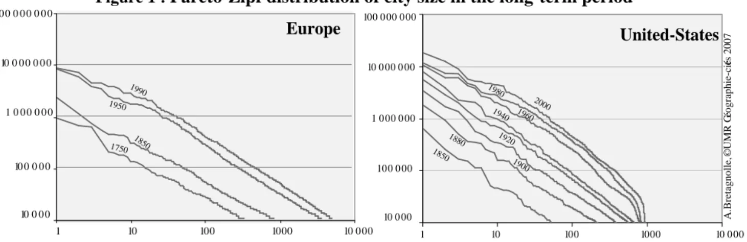
The lack of homogeneity of the spatial delimitation and statistical definition of urban areas over time is especially crucial for understanding why so many contradictions and interrogations remain in the literature on city size distributions. First, Guerin-Pace (1995) demonstrates that the number
and minimal size of cities that are selected for fitting different kinds of curves introduce a bias in the
estimation of their parameters. Second, the spatial delineation chosen for urban areas also matters when one try to conclude about historical trends. This explains for instance that on Figure 1, using harmonised data, we observe an increasing slope over time (demonstrating a trend towards a higher concentration at European scale) while when fixed territorial units are used, a decreasing slope can be found, as did M. Batty (2001) for population data from 1901 to 1991 in the case of Britain. The same observation can be made for United States between 1900 and 1950: with a 1990 delineation applied to prior decade, Black and Henderson (2003) obtain a stable or decreasing Pareto parameter, whereas we observe an increasing slope over time with our harmonized data-base (Figure 1 and Bretagnolle et al. 2008).
Figure 1 : Pareto-Zipf distribution of city size in the long-term period
10 0 0 0 10 0 0 0 0 1 0 0 0 0 0 0 10 0 0 0 0 0 0 10 0 0 0 0 0 0 0 1 10 100 1000 10 0 00 Europe A. Bretagnolle, © UMR G éographie-cit és 2007 1750 1850 1950 1990 10 0 00 100 0 00 1 0 00 0 00 10 0 00 0 00 100 0 00 0 00 1 10 100 1000 10 0 00 United-States 1850 2000 1880 1900 1920 1940 1960 1980
Not only the shape of statistical distributions of city size but the type of growth process which is assumed to explain them is depending as well on the quality of urban data. Many debates regarding the utility of the Gibrat’s model of urban growth (Gibrat, 1931) are made from data sets which were not previously harmonised (for instance, Gabaix and Ioannides, 2004). Although too simple and without any geographical theoretical basis (since excluding any interactions between cities), this model provides a first robust insight in the surprisingly persistent spatial pattern of the urban systems that are considered here over one or two centuries of strong demographic and economic growth (figure 2).
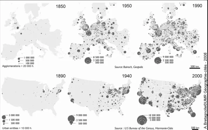
Figure 2 : Evolution of urban patterns (Europe and USA)
2. The generic model Simpop2
The SIMPOP2 model is designed for reconstructing the main features of urban dynamics from the simulated interactions between cities that are considered as the agents of the multi-agent system. It does not seek to reproduce in detail the real processes of an exchange market or a product cycle like a micro-economic model would. The stylised facts that we selected refer to higher order interactions which represent the asymmetries of trade between cities that were generated by their specialisation in a series of urban functions. Each urban function cover a bundle of economic activities that emerged at a given period as part of a specific innovation cycle and give an impulse to urban growth. A website is dedicated to the detailed presentation of the model, whose only main properties are recalled below (http://simpop.parisgeo.cnrs.fr).
2.1 Rules governing urban dynamics
Urban dynamics is summarised in three different ways in our model: first, the innovation cycles which played a major role in urban growth are selected and the urban functions are defined exogenously; second, the rules for the acquisition of new functions by the cities are expressed through a general process of hierarchical spreading of these innovations and a process of random or resource driven specialisation; and third, the inter-urban interaction space is modified according to innovations in transportation and communication techniques.
Out of the many cycles of innovation observed in the past, a few were retained for defining specialised urban functions. They were those which specifically selected a particular group of cities by specialising them in relation to the rest of the urban system. Four cycles meet this criterion:
- The long distance maritime and river trade, at the turn of the 12th-13th century in Europe, with the invention of money exchange and credit techniques allowing far-reaching exchanges, advancements in navigation and the major historic discoveries which partly modernised the specialised cities in this type of function and their exchange networks until the 17th century.
- The first industrial revolution, at the start of the 19th century, characterising either very small cities on mining fields and steel production, or large cities with a diversified economic base.
- The second industrial revolution with electricity and automobiles, at the end of the 19th century, characterised by urban specialisations in oil production, the construction of cars or tyres, and hydroelectric centres.
- The information technology revolution, in the mid 20th century, with the promotion of cities specialising in information production or new technologies and services to high level companies or tourism agencies.
These new specialisations are spread within the urban system according to two different types of rules in the model. One of the key hypotheses is based on the theory of hierarchical diffusion of innovations, formulated by T. Hägerstrand (1952) and tested many times on various urban systems, namely by A. Pred (1973). According to this theory and these observations, an innovation spreads within the urban system by leap-frogging down the urban hierarchy (and not according to a rule of geographic proximity as is the case for the spread of epidemics or agricultural innovations, for example). The biggest cities have infrastructures, social diversity and the functional level required to adopt new technical or social practices. In our model, the size of a city, measured by population or wealth, is therefore generally a prerequisite in the rules which allow it to possibly acquire a new function. This rule, which is never deterministic, may also be completed by other conditions, for example location or previous functional level (a city cannot gain a central function of a given level if it does not already have that of a lower level). When a specialised function is linked to the availability of specific resources, the cities where it develops are randomly selected among a subset of exogenously predefined locations (as coal basins or coastal areas). A city which has acquired a function and cannot find its place in the market will lose it after a few iterations, just as a declining market (for an innovation cycle in a phase of becoming commonplace then obsolete) can also lead to the disappearance of certain functions in the specialised cities.
Finally, the model systematically takes into account the major innovations in the transportation and information technologies, which have allowed a significant increase in the scope of interactions and renewal of exchange circuits. For each function level and type, a parameter controls the maximum range of the exchanges, which can vary over time depending on the data provided by historical documentation.
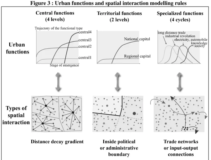
2.2 Urban functions and spatial interactions
Three types of urban functions are defined in the model according to the type of spatial interaction that they generate (figure 3):
- The central functions are those which depend on how a city exercises its centrality, i.e. those ensuring the servicing of a local population and environment through provision of goods and services. They remain principally within a limited proximity, thus the client city networks develop according to the gravity configurations. Two levels have initially been retained: the local level (Central 1, given to all cities, commercialises the agricultural surpluses of surrounding villages, within a radius of a few km, corresponding to daily exchanges), and the regional level (Central 2, producing commercial goods aimed at the cities’ demand, within a radius of some 70 km, corresponding to almost one day of travelling in Europe, in the pre-industrial era). In order to take into account the growth of the exchange scope in time and demand, (namely in more diversified consumables), two new levels of central functions have been introduced, Central 3 from the transportation revolution onwards, and Central 4 from 1900 onwards, with scopes which increase over time.
- The territorial functions are those which act within administrative limits: interactions are carried out in a determinist manner with all the cities included in the territory. Two levels have been retained: the regional level and the national level. The latter is only introduced when the kingdom borders are relatively stable (around 1500 in Europe) or when the States are institutionally constituted (around 1800 in the United States). Once the function has been acquired, the regional or national capitals take part of the wealth of the cities located within their territory, by levying a tax.
- The specialised functions are those driven by the different cycles of innovation. They are characterised by interactions which may be very distant. The cities which have the current specialised function have greater growth, however, the older the specialisation becomes, the slower the associated growth for the city. A city can attract a specialised function, either as a result of being drawn randomly (namely if it is part of an industrial field, oilfield or other), or because of its wealth or previous specialisation.
Figure 3 : Urban functions and spatial interaction modelling rules
2.3 Operating the market exchanges
A market exchange takes place between cities according to the functions they have, by matching supply and demand in sub-networks of cities, at each iteration of the simulation. Each iteration represents a period of ten years. Out of the 10 urban functions taken into account in the model, only the upper level central functions (2, 3 and 4) and the specialised functions are associated with an exchange market. Each of these functions is parameterised by productivity per employee and demand per inhabitant, which vary over time. Estimates of these parameters were computed from exogenous variables which are extracted from work of historians or economists (such as Mitchell, 1992 or Bairoch et al., 1988). The values are orders of magnitude rather than exact values (which it would be impossible to calculate before the 19th century). The parameter values respect two constraints: the hierarchy between the functions (the demand or productivity per inhabitant is weaker for central function 2 than for central function 3, etc.) and temporal growth (over time, both demand and productivity increase). Furthermore, a third exogenous parameter helps to compute the proportion of workers per function when this appears in a city.
At the start of each iteration, the model calculates the supply (productivity per inhabitant multiplied by the number of workers in this function) and demand (demand per inhabitant multiplied by the total population of the city) for each city and each function. A potential exchange network is then created, i.e. the list of cities located within the range currently associated with the function and which have a demand. For the specialised functions, only those cities possessing certain functions may be clients: for example, the cities which don’t have the regional commercial function, called central 2 in the model, cannot buy goods produced from long distance trade (cycle 1). This method allows the relatively selective nature of these exchanges to be taken into account.
Once each producer city has created its potential network, a second mechanism intervenes to select the partnerships, i.e. the buyers and sellers who will effectively make an exchange. The producer distributes its supply in proportion to the distances separating it from potential buyers, according to a gravity model (the closer the buyer, the more it is favoured). Conversely, the potential buyer
distributes its demand among the different producers in proportion to the size of their respective potential client network (the more potential clients a producer has, i.e. the better its position in relation to the urban networks, the more it will be favoured). For each potential buyer/seller pair, the minimum between the supply proposed and the demand addressed is then calculated, and it based on this that the actual exchanges are made. The process is repeated until the supply can no longer be met by the demand and vice versa.
2.4 Computing economic and demographic growth
At the end of each iteration, the number of workers in each function, the total population and total wealth of each city are reassessed. Three mechanisms are involved in calculating the demographic growth.
The first is not dependent on the exchange market and consists of allocating part of the
demographic growth observed in the past, regardless of the city’s success in the exchange market,
its size or any other consideration: each city receives exactly the same rate, at a given period. It involves accounting for the current demographic trend, which may be marked by crises (epidemics, wars, economic recessions) or, conversely, by periods of intense urbanisation (urban transition, rural exodus etc.). The proportion of demographic growth which we include in the model is a parameter which may grow over time: the lower it is, the stronger the growth generated solely by the exchange market, which is translated by a greater differentiation in city sizes because of competition mechanisms.
A second mechanism consists of adjusting, upwards or downwards, the number of workers per activity sector for each city according to the result of its exchanges, thus reflecting the more or less positive attractiveness on the labour force. If the city has sold all its supply in a certain sector while demands by potential client cities are not met, the number of workers in the function is increased so as to better meet the demand in the following iteration. Conversely, if a city has not been able to sell all its produce, the number of its workers is decreased, according to the amount of unsold supply. Two parameters are used to implement this mechanism, the market potential (which assesses the unmet demand or, conversely, the unsold produce and the total number of workers to be added or removed to perfectly adjust to the demand for each city and function) and the market reaction speed (which determines, modulo a random number, the proportion of workers actually added or removed in relation to this total. The greater this proportion, the quicker the city adapts to the result of the exchange. This reaction speed is linked to the more or less high speed of the information circulating between the cities and which allows workers to migrate quickly to any given attractive location; it varies according to the advancements made in information technology in recent centuries).
Finally, the third mechanism consists of a proportion of demographic growth generated by the
profits of the exchange. Compared to the second mechanism, which indifferently favours the cities
possessing central functions or specialised functions, this mechanism places great emphasis on the theory of unequal exchange: a city which chooses (and takes the risk) to invest in leading sectors is likely to gain more profits than a simple regional commercial centre. These profits will then be translated, in the more or less long term, by a greater attractiveness on the labour market. This mechanism is implemented using two parameters, the plus value on each function and the market
return on demographic growth. At the end of each iteration, the number of production units sold by
the city is converted into the number of wealth units, taking into account, by using the plus value parameter which varies according to the functions, the most significant profits gained from the sale of specialised, innovative goods. The total wealth of the city is recalculated, and from this we deduct relative enrichment compared to the previous iteration. This enrichment is transformed into a multiplicative coefficient applied to the average rate of current demographic growth (the equations of the model can be found in appendix 1 and are more detailed on the website http://www.simpop.parisgeo.cnrs.fr/theGenericModel/rules.php).
3 Simulating the European urban system (1300-2000)
The simulation starts at a moment where the long-distance exchanges are reactivated in Europe. During the 12-13th centuries, for example, the cities of the Hanseatic league traded with those of northern Italy, through stopover points established in France (Champagne trade fairs) then in
Germany (thanks to the opening of alpine passes). The distribution of cities is already quite dense, with an average of one city every 20 km, except in forested, moor land and mountainous areas. A large part already existed during the Roman era, with the exception of new cities resulting from religious settlements or the vast clearings during the 12th-13th centuries in the west, and the 15th-16th centuries in the east. The form of the urban hierarchy is hard to deduce from historic sources which do not contain much information on the small localities. For the largest, the estimations of Paul Bairoch list 170 cities with more than 10 000 inhabitants, out of which 3 exceed the 150 000 inhabitants (Paris, Granada and Venice). All these characteristics allow the initial situation of the implemented model to be created.
3.1 Simulations on a theoretical urban network
In order to concentrate on the generic rules governing urban growth, we conducted our first simulations from an initial simplified situation, in which the locations are randomly scattered inside a square. To do this, a regular triangular (Christallerian) pattern was generated, with a distance of 35 km between each point, giving 5000 points (the current number of cities in Europe) within a square of 5 million km2(Table 1). Out of these 5000 cities, 1000 are activated from 1300 (i.e. the approximate number of cities existing at that time). The other 4000 are activated over the following centuries, drawn at random. The initial cities received a randomly selected population in a lognormal distribution whose parameters (average, standard deviation and minimum population) are identical to those calculated for the observed distribution _in 1300. The initial functions given to the cities in 1300 are the territorial functions (chief towns in 1300 in the west and in 1500 in the east, capitals in 1500), some central functions (level 1 for all cities and level 2 for some of the larger ones selected randomly), and the long distance trade specialisation. The latter function was randomly allocated to the large cities located at the southern and western edge of the square (representing the Mediterranean and the Atlantic) and in a north-west/south-east diagonal (representing the intermediary stopover points between the cities of the Hanseatic region and those of northern Italy). From 1800 onwards, two industrial fields are activated in the northern half of the square (in the west: mining basins of the Rhine and Ruhr, in the east: the Silesia basin). Inside these fields, some of the cities obtain the industrial function, randomly drawn among the smaller localities which only have central function of lowest level.
A multi-scale validation protocol (designed by Hélène Mathian, UMR Géographie-cités) help for calibrating the model, from the macrogeographic scale (computing total population, total wealth, number of cities per size class and slope of the rank-size graphs, share of employees per function) to the mesogeographic scale (trajectories of cities aggregated by regions, or by urban function) and microgeographic scale (maximum size at each time, trajectories of individual cities). The model satisfactorily reproduces the growth of the system’s total population, even during times of recession (the Great Plague in the 14th century) or, conversely, intense urban expansion. However, simulating correctly the urban growth during the industrial revolution and urban transition of the 19th century requires a multiplication by 3 of the values of the growth parameters linked to the market (Pumain et al. 2009). The slope of the rank-size distribution grows coherently (Table 2).
Table 2: Evolution of inequalities in city sizes in Europe Observed Simulated Slope* R2 Slope R2 1800 0.69 0.99 0.75 0.98 1850 0.77 0.99 0.78 0.98 1950 0.91 0.99 0.89 0.98 2000 0.94 0.99 0.94 0.98
* Estimated slope of a fitted rank-size curve to the distribution of city sizes
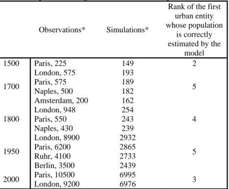
However, none of the numerous correct simulations was able to produce a sufficient size for the biggest cities, while the total number of cities in the largest size category is correct (cities of more than 100 000 inhabitants between 1500 and 1900, then cities of more than 200 000 inhabitants etc.). Table 3 shows that the population of the biggest cities is only well simulated under a certain rank
(the second in 1500, the fifth in 1700 etc.). For example, in 1500, the observed population of the biggest city is 225 000 (Paris) and 149 000 according to the simulations, despite many trials when calibrating the parameters. This means that the functions included in the model (long distance trade, national or regional capital, first and second industrial revolutions) are not enough to generate such growth, even when the city concentrate them all at the same time. These cities share the same characteristic, regardless of the period concerned: from the Middle Ages, their sphere of influence largely exceeds the European context, for example for Naples (capital of the Kingdom of the Two Sicily and focusing on the Mediterranean) or for Paris (place of international finance during the time of the Lombard bankers) and later London (dominating Indian and American trade). The simulations suggest introducing a new function into the model, which could be called following F. Braudel (1979) a “world-city” function and which would characterise a very small number of cities strongly connected to the world outside the system.
Table 3: Population of largest urban entities in Europe
Observations* Simulations*
Rank of the first urban entity whose population is correctly estimated by the model 1500 Paris, 225 149 2 1700 London, 575 Paris, 575 Naples, 500 Amsterdam, 200 193 189 182 162 5 1800 London, 948 Paris, 550 Naples, 430 254 243 239 4 1950 London, 8900 Paris, 6200 Ruhr, 4100 Berlin, 3500 2932 2865 2733 2439 5 2000 Paris, 10500 London, 9200 6995 6976 3
* population in thousand. Sources : Bairoch et al. 1988, Moriconi-Ebrard 1994. 3.2 Geo-referenced simulations
Another set of simulations considered the real locations of the cities with their population and functions for defining the initial situation in 1300. The aim was to clarify, by comparing them with the theoretic simulations, the role of geographic configurations and heritages (path dependence, according to Brian Arthur’s (1994) expression) in the urban growth. Indeed, the situation in 1300 is already integrating a complex history, contrasting the dense and highly specialised urban regions (in northern Italy, north-western Europe and southern Spain) and other still deeply rural regions (Scandinavia, Poland and Central Europe).
The initial allocation of functions was done according to the same mechanisms which were used for theoretic Europe2. All the cities obtain Central function of level 1 in 1300 and some of them (the biggest) Central function level 2 (regional trade between the cities). The capitals are introduced from 1500 onwards, a period characterised by a grouping of authority within relatively stable national borders. The regional capital function is allocated to about one hundred cities according to size criteria). The “long distance trade” specialisation is given to about fifty cities identified from historic sources. These are Mediterranean cities which trade with the Orient and the Maghreb, cities of the Hanseatic League located on the Atlantic and Baltic coast (trading fur and wood with the
2
The historical sources that have been used in this work are : Bardet J.-P., Dupaquier J., 1997, Histoire des populations de l’Europe. 1 – Des origines aux prémices de la révolution démographique, Paris, Fayard, 660 p. Pinol (dir.), Histoire de l’Europe Urbaine, tome 1 : De l’antiquité au XVIIIe siècle, Paris, Seuil. Bairoch P., 1997, Victoires et déboires :
east), and intermediary stopover points in France and in Germany. Added to this list are other Atlantic cities already involved in the international exchange circuits in 1300 (Portugal, England), or certain European capitals (Paris, Prague). The specialisations resulting from the first industrial revolution are partly given to small towns located in the heart of mining and metallurgic fields (Midlands, Franco-Belgian basin, Galicia, Silesia, Ruhr). In the model, one third of the cities which obtain the industrial function are randomly chosen inside these polygons, from those who only have Central function of level 1.
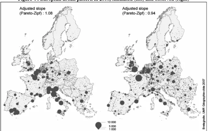
In order to test the role of the initial situation in the growth of the urban systems, we used the same parameters in the two types of simulations, i.e. those calibrated for theoretic Europe. The results are noticeably different (Figure 4). Firstly, the total population is largely underestimated. At the same time, the distribution of city sizes is more contrasted in the geo-referenced simulation (slope of 1.08, Figure 4) than in reality and the theoretic model (slope of 0.94 in both cases). Given that the parameters of growth (demographic or associated with the market) are strictly the same, these differences are a result of more intense competition mechanisms in the real simulation than in the theoretic simulation: for cities located in densely urbanised areas, growth is limited by the proximity of neighbouring cities, and for cities in isolated locations, declines are linked to their isolation compared to the main exchange circuits.
Figure 4 : European urban pattern in 2000, simulated (left) and observed (right)
Furthermore, the results show that the urban growth remains largely underestimated in the northern half of Europe (southern England, Scandinavia, Germany, Poland), while in the south, the cities of southern Spain and northern Italy have remained at the top of the hierarchy since the Middle Ages. The shift in Europe’s centre of gravity, from the south to the north (Braudel, 1979, de Vries, 1984), is not reproduced correctly by the simulation, which gives too much weight to historic heritage. This result prompts us to rethink this major historic growth within the context of the modelling: which rules or parameters should be introduced into the model to correctly simulate the relative decline of vast urban regions in southern Europe and the emergence of new areas in the north? Should we namely introduce differentiation mechanisms which are recorded within national borders, which have not yet been taken into account in the model? Additional research is currently being conducted regarding this.
Indeed, one last observation shows the role of national governance in the growth of European cities. Figure 4 states that the hierarchical relationships between the sizes of cities in France or Spain are incorrectly reproduced by the simulation. These are two countries with a centralised tradition,
whose capitals have experienced significant developments compared to other cities. However, the initial situation and the rules of the model do not take into account the governmental styles of each of the different countries. The model shows the strength of the structuring processes which underlie the growth of the European urban system on a national scale.
4. A new version of the model for United States
The American urban system is very different from that depicted for Europe and belongs to a second type of system, that of newly settled countries, where the urban population was formed in successive waves (Pred, 1966, 1973 and 1977, Dobkins, Ioannides, 2001). The cities are on average much more spaced out than in Europe (one approximately every 50 km in 2000). At the time of the railroad, most cities were born with spheres of influence which covered territories much greater areas than the natural means of transport which sustained the first developments of European cities. Another difference is the very dissymmetric nature of the urban pattern - dense in the east but very sparse in the west, because of the vast desert and mountainous areas.
4.1 An initial situation including a new mechanism: urban frontier
In the United States, cities that emerged between 1650 and 1790 are activated according to their order of appearance in the historic sources with their initial population3. An urban frontier mechanism then controls the spread of the cities according to the number of cities activated at each time and the perimeter in which cities are activated randomly. After 1910, cities are drawn randomly from all over the country, like in the European model.
The functions allocated to the cities in their initial situation are the same as in the European model. All the cities obtain the Central function level 1 and only some, selected randomly, benefit from an upper level central function. The allocation of territorial functions is articulated on the urban frontier mechanism: the capitals of each state receive this function as soon as they are set up by the urban frontier, while the federal capital emerges from 1800. The “long distance trade” specialisation is allocated according to three waves: the first describes the large Atlantic ports (from 1740); the second (1810-1850) is represented by maritime or river ports, stimulated by slave trade (Baltimore, New Orleans) and mechanical agriculture (Cincinnati, St. Louis, Chicago); finally, the third wave is made up of large Pacific ports which emerge as such from the 1860s (Seattle, San Francisco, Portland, Los Angeles). From 1830 onwards, some of the cities located in the polygon stretching from the Great Lakes region to the Atlantic coast, receive the manufacturing function. A second wave is made up of cities located near goldfields or other metal fields in the west. Finally, between 1890 and 1930, some cities located within the southern and western polygons (oilfields) are selected to receive the specialised Cycle3 function (second industrial revolution).
In a first simulation, we applied the parameters calibrated for theoretic Europe to this initial situation, as we had previously done for real Europe. Not surprisingly, the results were extremely mediocre, but their analysis was rich in information for establishing a list of fundamental differences between the two types of urban systems. Firstly, the total population of American cities is widely underestimated, from the start of the 19th century, primarily due to the market mechanisms: the proportion of workers decreases in each function, whether central or specialised, for most of cities. Second, the population remains primarily concentrated in the eastern cities, whereas those in the west and south are not achieving any growth. Finally, the large regional metropolises (even those in the east) are characterised by much weaker growth than that observed.. Starting with the pre-industrial period, we parsimoniously modified the rules resulting from the Europe model, based on a specific diagnosis of the inadequacies in the simulation results. In the end, four new rules were necessary to obtain satisfactory simulations. These rules, in a way,
3
The historical sources used for United states are : Greene E. B. et Harrington V. D. (1932, reed. 66), American population before the Federal Census of 1790. Gloucester, Massachusetts. Hugill P. (1993), World Trade since 1431: Geography, Technology and Capitalism, Baltimore and Boston, The John Hopkins University Press. Kim Sukko (2007), “Immigration, Industrial Revolution and Urban Growth in the United States, 1820-1920. Factors Endowments, Technology and Geography”. NBER Working Paper No. W12900 Available at SSRN: http://ssrn.com/abstract=963734. Vance J. E. (1990), Capturing the Horizon. The Historical and Geography of Transportation since the Sixteenth Century. Softshell Books edition. Chudacoff H. (1981), The evolution of American Urban Society, Englewood Cliffs,
summarise the fundamental specificities of the American urban system compared with that of Europe.
4.2 Identifying specific rules for the United States
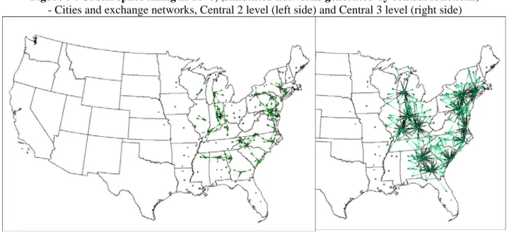
The simulations using the parameters calibrated for Europe cannot generate the mushrooming development of the cities created on the urban frontier. They remain too small to be able to adopt regional level central functions or specialised functions. They deteriorate over the decades following their creation, instead of growing and integrating into the exchange market as they had done in the past. It is because in reality these cities of the urban frontier4 appeared even before surrounding land has been made usable. They emerged as commercial outposts, from which the population radiates, creating a market around them and increasing the land value. In turn, the expansion of the agricultural frontier stimulates the growth of these commercial nodes. A new mechanism, called Urban frontier growth was thus introduced into the model and provides (using one parameter) a greater current demographic growth for the cities located in front of the urban frontiers. This mechanism is activated between 1790 and 1900.
A second rule has to be introduced: behind the urban frontiers, the cities acquiring regional level central functions (central 2 and central 3) are also encountering significant decrease in the simulations in the first half of the 19th century. Their decline results of a considerable stock of unsold products, due to the lack of client cities within range at the time. Although this range was already extended to 100 kilometres between 1830 and 1840 (compared to 70 km in Europe) to take into account the railway network and steamboats circulating along the rivers or canals, it is not enough to enable the cities (still very few, as they are less than 100 urban centres) to provide level 2 goods and services to the entire colonised territory (which stretches over 2000 km between the east coast and the Mississippi). Consequently, the level 2 and 3 central functions were introduced later
than they were in Europe, in 1850 for Central2 and 1870 for Central3 in order to enable the take off
of their stock of potential consumers. Figure 5 shows that, in 1870, the customer networks of these cities develop correctly. This reflect the specific rationale of the early emergence of cities in the US that is different to that existing in Europe: while in the latter, most of the cities emerge on an essentially local trade (Bairoch, 1985, Hohenberg, Lees, 1992), it is essentially the specialised functions which create the growth of American cities until 1850, according to the Vance mercantile theory (Vance 1970).
Figure 5 : Urban space filling in 1870, (simulated networks generated by central functions) - Cities and exchange networks, Central 2 level (left side) and Central 3 level (right side)
A third rule is designed for correcting the evolution of specialised cities, which also suffer from a lack of customer cities in the first half of the 19th century. By keeping the same productivity and
4
the same demand per inhabitant parameter as in Europe, the long distance trade cities experience masses of unsold items. Once again, the model enlightens a major specificity of the United States urban system, i.e. the decisive impact of the exchanges with the world outside the system during its stage of emergence. Right throughout the 18th century and the first half of the 19th century, the Atlantic ports export fur, cereals, fish and wood to Europe. This strong external link is then maintained through the cities in the Gulf of Mexico and the Mississippi ports (exchanges with the Caribbean and Canada), then the cities of the west coast, whose main focus is Asia. In order to take into account this boost provided by the international environment, a new parameter was introduced into the United States model. The latter sets the additional demand (representing massive investment and immigration) quantity necessary for the long distance trade function to develop correctly, and in return awards the financial gains generated by these sales. With this same diagnosis being conducted for the following innovation cycles, these were supported by a similar mechanism: an international demand was incorporated to allow for simulating the exceptional growth of the cities specialised in the industrial revolution (for example Pittsburgh, which went from 12 000 inhabitants in 1830 to 450 000 in 1900), those of the second industrial revolution (for instance San Antonio in Texas, which went from 53 000 inhabitants in 1900 to 500 000 in 1950) and those of the ICT and tourism revolution (see Orlando in Florida, which went from 36 000 inhabitants in 1940 to 430 000 in 1970).
These three modifications in the rules of the model enable it to properly simulate the total urban growth, but not its spatial distribution. Indeed, another characteristic of American cities is the very close correlation existing between each innovation cycle, the associated fields of resources and the emergence of new regional metropolises. Most of the cities which suddenly emerge during an innovation cycle are concentrated in very specific regions: the north Atlantic coast at the start of the 19th century (New York, Philadelphia and Boston), the south Atlantic coast and the Mississippi system in the mid 19th century (Baltimore, Cincinnati, New Orleans, St. Louis, Chicago), the cities of the industrial hub in the second half of the 19th century (Pittsburgh, Chicago or Cleveland), those of the gold rush at the end of the 19th century (San Francisco), the oil boom (Texas, California) and the land speculation from 1900 to 1930 (California then Florida, Arizona and New Mexico). For each of these identified resource basins, an initial boost was given to the cities activated there. A new parameter stands for a share of the external demand addressed to these specialised functions that is directly allocated to cities of the corresponding resource fields during the first decades of each new cycle.
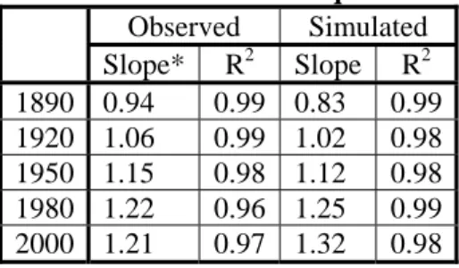
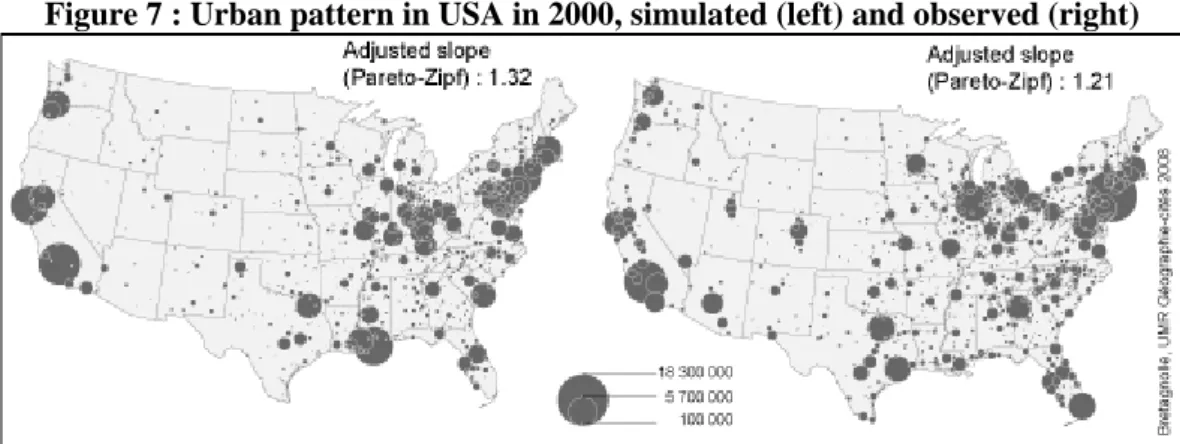
With these new rules, the situation allows a much better calibration (figure 7 and table 4): not only the macrogeographic figures, but the regional developments at meso level as well as the trajectories of individual cities at a micro level (New York or other eastern cities such as Philadelphia or Boston remain at the head of the system, whereas the metropolises of regions located in the west then the south propelled themselves to rejoin them at the top of the hierarchy).
Table 4: Evolution of inequalities in city sizes in USA Observed Simulated Slope* R2 Slope R2 1890 0.94 0.99 0.83 0.99 1920 1.06 0.99 1.02 0.98 1950 1.15 0.98 1.12 0.98 1980 1.22 0.96 1.25 0.99 2000 1.21 0.97 1.32 0.98
* Estimated slope of a fitted rank-size curve to the distribution of city sizes
Moreover, just like for Europe, a rule favouring the specific growth of certain metropolises, according to a “world-city function” is yet to be introduced: New York compared to pioneer cities on the east coast, Chicago compared to cities of the industrial hub, Los Angeles compared to the cities of the west coast are the three nodes that are selected. These cities actually form the main gateways, the necessary ties between the United States and the other world-cities in Europe, Asia or the rest of America.
Figure 7 : Urban pattern in USA in 2000, simulated (left) and observed (right)
Conclusion
By using a multi-agent model, we have presented an original method for specifying the comparison between different types of urban systems in the world. First of all, the simulations validate the principle of a generic model of the evolution of urban system, that simulates the emergence of their common properties at a macrogeographic level: the importance of interactions in the cities’ demographic and functional dynamics, the role of innovation cycles in urban growth, the effect of increasing the range of exchanges on the urban hierarchy.
However, the modelling also underlines and measures differences previously observed in a qualitative way between the different types of settlement systems, linked to their historical process of space filling. For the United States, the temporal coincidence between the implementation of the inter-urban exchange system and the transport revolution, which instantly allows for exchange scopes four times larger than those characterising the European urban network during the system’s emergence phase, gives specialised functions a driving role in urban growth. The low number of cities (and therefore potential clients for regional level central functions) is thus compensated by the possibility of selling specialised produce to all the regions of a country the same size as Europe and to the rest of the world. A second characteristic of American cities, also linked to the mass mobilisation of information and transport technologies, is the very intense mobility within the labour market. The exceptional trajectories of small towns, which display annual growths of 5 to 10% and in just a few decades become a national or international metropolis, are only possible at the price of extremely large influx of migrants, from abroad as well as different regions within the country. This very high adaptability of labour was shown in the literature and is clearly apparent in the parameters of the model, whose values are much greater than for Europe. Finally, one last characteristic is linked to the size and geographic diversity of the country, which allows for higher levels of urban specialisation because these cities instantly find numerous markets thanks to the efficiency of transport systems. They can then diversify their production and become competitive in other sectors of activity.
Because it is operating over long periods of time, the Simpop model may help to answer many questions that are now raised in large developing countries as India or China, where urbanism still has to expand dramatically. Its ability to reproduce the structuring of urban systems of industrialised countries during the urban transition represent a useful tool for exploring the possible futures in these rapidly urbanising countries- provided of course the necessary relevant adaptation of rules and context parameters. In industrial countries, the 21st century opens a new stage in the history of system of cities: the urban transition is now over, after two hundred years during which it completely transformed our way of inhabiting the planet, from a scattered and rather homogeneous rural settlement system into a very concentrated, hierarchical and heterogeneous urban system. What future can be expected for cities in developed countries, where there is no longer migration from rural areas or local demographic growth for sustaining the cities development? Will population and activities continue to concentrate in the largest metropolises? Are the small and medium size towns condemned to decline and disappear, as did so many villages in the past? Will new means of communication – the Internet and its successors – diminish the advantages of cities (for instance in terms of innovators per capita) as the need for strong regional interaction seems no
longer of the essence in a world where everybody is theoretically related to everybody? This very often suggested option for the future has to be confronted to facts, before imagining scenarios for a predicting use of the Simpop model.
Acknowledgments: We gratefully acknowledge support from the European Commission (ISCOM project), and the French CNRS and MNRT (ACI Systèmes complexes en SHS)
Appendix1 : Equations of the SIMPOP model
The total population at t+1 is function of 3 components :
(
t)
i t i t i t i t iP
P
P
P
P
+1=
+
Δ
1+
Δ
2+
Δ
3( )
1
Demographic trend t i t h t t iG
P
P
=
∗
∗
Δ
1α
( )
1 t hG
represents the global demographic trend at time t in the region h andα
t a parameter that evolves over time between 0 and 1 and that weights the global demographic trend of the cities.( )
2
Evaluation of labour force attractivity for each urban function k of city i : First, the variation of active population between t and t+1 for the sector k is evaluated by:t ik t ik t t ik
s
PotM
P
→ 1+=
Where
P
ikt→ t + 1 represents the variation of workers in sector k, based on the potential of the trade network of this sector for the city i (i.e.PotM
ikt ). That corresponds more or less to the demand of the network of customers for the sector k, at time t, after the trading process. If there are unsold goods, the potential will be negative, reversely if there is unsatisfied demand, it will be positive.t ik
s
is a parameter which probability follows a normal distributionN
(
m
sσ
s)
. For the short term simulations, it may be interpreted as the “speed of adjustment”.Then, the variation of active population due to the market adjustment is given by:
∑
→+ =Δ
k t t ik t iP
P
1 2( )
2( )
3
Market returns :The third part of the evolution of the population is linked to an attractivity due to the enrichment of the city:
(
t)
t i t t iw
W
P
min
;
0
/
3∗
Δ
Δ
=β
( )
3 t iw
is the wealth of the city i at time t.t i t i t i
w
w
w
=
−
Δ
+1measures the balance of wealth of the city i at time t and
W
t the maximum attractivity of the system at time t.t
β
is the weight given to this component of the population variation at time t. If there is no enrichment there, this component has no effect.References
Arthur W. B. 1994, Increasing returns and path dependence in the Economy, Ann Harbor, Michigan: University of Michigan Press.
Bairoch P., 1985, De Jericho à Mexico, villes et économie dans l’histoire, Paris, Gallimard, Arcades, 705 p.
Bairoch P., Batou J., Chèvre P., 1988: La population des villes européennes. Banque de données et
analyse sommaire des résultats: 800-1850. Centre d'Histoire Economique International de
l'Université de Genève, 339 p.
Batty M., (2001) ‘Polynucleated urban Landscapes’, Urban Studies, Vol.38 No.4 / 635-655
Berry B.J.L. 1964, Cities as systems within systems of cities. Papers of the Regional Science
Association, 13, 147-163.
Black Duncan, Henderson Vernon 2003, “Urban evolution in the USA”. Journal of Economic
Geography 3, 343-372.
Bourne L. Sinclair R. Dziewonski K. (eds) 1984, Urbanization and Settlement Systems: International Perspectives. Oxford, Oxford University Press.
Braudel F. 1979, Civilisation matérielle, Economie et capitalisme, XVe – XVIIIe siècles (tomes 1, 2
et 3), Paris : A. Colin.
Bretagnolle A., Pumain D., Rozenblat C. 1998, Space-time contraction and the dynamics of urban systems ». Cybergeo, 61, http://www.cybergeo.eu/index373.html , 12 p.
Bretagnolle A., Mathian H., Pumain D., Rozenblat C. 2000, Long-term dynamics of European towns and cities : toward a spatial model of urban growth (1200-2000). Cybergeo, 131,
http://www.cybergeo.eu/index373.html, 17 p.
Bretagnolle A., Paulus F., Pumain D. 2002, Time and space scales for measuring urban growth. Cybergeo 219, http://www.cybergeo.eu/index3790.html, 12 p.
Bretagnolle A., Daudé E.., Pumain D. 2006, From theory to modelling: urban systems as complex systems. Cybergeo 335, http://www.cybergeo.eu/index2420.html 26 p.
Bretagnolle A. Pumain D. Vacchiani-Marcuzzo C. 2007, Les formes des systèmes de villes dans le monde, in Mattei M.-F. Pumain D. (eds) Données urbaines 5, Paris, Anthropos-Economica, 301-314.
Bretagnolle A., Giraud T., Mathian H. 2008, L’urbanisation des Etats-Unis, des premiers comptoirs coloniaux aux Metropolitan Areas (1790-2000). Cybergeo, 427.
Bretagnolle A., Pumain D., 2008, Comparer deux types de systèmes de villes par la modélisation multi-agents (Europe, États-Unis), in Zwirn H. Weisbuch G ; (eds), Complexité en Sciences
Humaines et Sociales, Paris, Vuibert.
Bura S. Guérin-Pace F. Mathian H. Pumain D. Sanders L. 1996, Multi-agent systems and the dynamics of a settlement system. Geographical Analysis, 2, 161-178 .
Cattan N. (ed) 2007, Cities and networks in Europe. A critical approach of polycentrism. John Libbey Eurotext.
Christaller W. 1933, Die zentralen Orte in Süddeutschland. Jena, Fisher.
Dobkins L.H.., Ioannides Y. M. 2001, Spatial interactions among U.S. cities: 1900-1990. Regional
Science and Urban Economics, 31, 701-731.
Duranton G. Puga D. 2004, Microfoundations of urban agglomeration economies, in Henderson J.V. and Thisse J.F. (eds) Handbook of Urban and Regional Economics, North Holland, vol. 4. Frenken, K., Boschma, R.A. 2007, A theoretical framework for evolutionary economic geography: industrial dynamics and urban growth as a branching process. Journal of Economic Geography, 7(5): 635-649.
Fujita M., Krugman P., Venables A. 2001, The spatial economy, Cambridge, MIT Press.
Gabaix X. 1999, Zipf’s law for cities: an explanation. Quarterly Journal of Economics, 114, 739-767.
Gabaix X. Ioannides Y.M. 2004, The evolution of City size distributions, in:
Handbook of Regional and Urban Economics, volume 4, Chapter 53, V. Henderson and J-F. Thisse
eds, North-Holland, p.2341-2378.
Gibrat R. 1931, Les inégalités économiques. Paris, Sirey.
Guérin-Pace F. 1995, Rank-size distribution and the process of urban growth. Urban Studies, 32:551-562
Hägerstrand T., 1952, The propagation of innovation waves, Lund, The Royal University of Lund, 20 p.
Hall P., 1998, Cities in civilisation: Culture, Innovation, and Urban order. London, Weidenfeld and Nicolson.
Henderson J.V. 1985, Economic theory and the cities. Academic Press.
Hohenberg P.M. Lees L.H. 1992, The Making of Urban Europe, 1000-1950,Harvard Studies in Urban History. Cambridge, MA: Harvard University Press
Janelle D. 1968, Central place development in a space-time framework. The Professional
Geographer, 20, 5-10.
Mitchell B. R. (1992), International Historical Statistics, Europe 1750-1988, Basingstoke : Macmillan.
Moriconi-Ebrard F., 1994, Géopolis, Pour comparer les villes du monde, Paris, Anthropos, Economica, Collection Villes, 246 p.
Nitsch V., 2005, Zipf zipped. Journal of Urban Economics, 57, 86-100.
Paulus F. 2004, Coévolution dans les systèmes de villes : croissance et spécialisation des aires
urbaines françaises de 1950 à 2000. Université Paris 1, thèse de doctorat.
Pred, A.R. 1966, The Spatial Dynamics of U.S. Urban Industrial Growth, 1800-1914. Harvard University Press, Harvard, MA.
Pred A. 1973, Urban growth and the circulation of information : the United States system of cities,
1790-1840. Cambridge (Mass.), Harvard University Press.
Pred A., 1977, City systems in advanced economies, London, Hutchinson.
Pumain D. 1998, Urban Research and Complexity, in Bertuglia C.S., Bianchi G., Mela A. (eds) The City
and its Sciences, Heidelberg, Physica Verlag, 323-362.
Pumain D. 2000, Settlement systems in the evolution. Geografiska Annaler, 82B, 2, 73-87.
Pumain D. 2004, “An Evolutionary approach to Settlement Systems”, in Champion, Hugo (eds), New
Forms of Urbanization, Beyond the Urban-Rural Dichotomy. Aldershot, Ashgate, 231-247.
Pumain D., (ed) 2006, Hierarchy in natural and social sciences, Dordrecht, Kluwer.
Pumain D., Saint-Julien T., 1984, Evolving Structure of the French Urban System. Urban Geography, vol.5, n°4, 308-325.
Pumain D., Saint-Julien T., Cattan N., Rozenblat C., 1991, The statistical concept of city in Europe. Luxembourg, Eurostat, 72 p.
Pumain D. Saint-Julien T. 1996 (eds), Urban networks in Europe. Paris, John Libbey-INED, Congresses and Colloquia, 15, 252 p.
Pumain D., Paulus F., Vacchiani-Marcuzzo C., Lobo J., 2006a, An evolutionary theory for interpreting urban scaling laws. Cybergeo, 343, http://www.cybergeo.eu/index2519.html .
Pumain D., Bretagnolle A., Glisse B. 2006b, Modelling the future of cities. Proceedings of the
European Conference on Complex Systems (ECCS’06, Oxford), http://halshs.archives-ouvertes.fr/halshs-00145925/en/.
Pumain D., Sanders L., Bretagnolle A., Glisse B., Mathian H. (2009), The future of urban systems : exploratory models, in D. Lane, D. Pumain, S. Van der Leeuw, G. West (eds), Complexity perspective in innovation and social change. Springer, pp. 351-359.
Robson B.T. 1973, Urban Growth, an approach. London, Methuen.
Rozenblat C. Cicille P. 2003, Les villes européennes. Analyse comparative. DATAR et Dcoumentation française.
Sanders L. Pumain D. Mathian H. Guérin-Pace F. Bura S. 1997, SIMPOP: a multi-agent system for the study of urbanism. Environment and Planning B, 24, p. 287-305.
Sanders L., Favaro JM., Glisse B., Mathian H., Pumain D. 2007, Intelligence artificielle et agents collectives: le modèle Eurosim. Cybergeo, 392.
Taylor P.J. Derruder B. Saey P. and Witlox F., 2006, Cities in Globalisation, London, Routledge. Vance J. 1970, The Merchants’World: the geography of wholesaling. Prentice-Hall, Englewood Cliffs, New Jersey.
de Vries J. 1984, European urbanisation 1500-1800. London, Methuen.