Distribution of the chi-squared test in nonstandard situations

Biometrika (1977), 64, 1, pp. 115-21 Printed in Great Britain

Distribution of the chi-squared test in nonstandard situations

B Y LUCIANO MOLTNABI

Department of Statistics, University of California, Berkeley, and Eidgenossische Technische HochschiUe, Zurich

SUMMARY

The distribution of the x% t68^ under the null hypothesis is studied, when the parameters are estimated by the method of moments. A general formula, applicable also to other situations, is given. Three examples are studied in more detail and numerical results are given, indicating how unsafe it can be to use a #2 distribution with a number of degrees of freedom smaller than or equal to the number of cells.

Some key words: Chi-squared teat; Distribution of quadratics forms; Goodness of fit.

1. LNTBODTJOTION

The standard theorem on the asymptotic distribution of the

=

Si

np< '

is given, e.g. by Cramer (1946, p. 427) or Rao (1973, p. 391), and rests on several assumptions about the true distribution of the observations and the estimators of any unknown parameters. These assumptions are not satisfied in practice mainly for the following reasons:

(a) estimators are obtained from the ungrouped data rather than from the grouped observations;

(b) the cells are often random, i.e. are determined by a first look at the observations; (c) the method of estimation is not efficient.

Points (a) and (b) were discussed by Chernoff & Lehmann (1954) and by Watson (1958). In both cases it is safe to consider X* as having a %2 distribution with k — 1 degrees of freedom,

the level of significance being then underestimated.

A discussion of (c) for the method of moments is given. I t seems that the formulae derived could be easily applied to other estimates. It turns out that in some cases, not at all 'patho-logical' ones, it would be very unsafe to use a xi distribution with k— 1 degrees of freedom.

The following notation will be used in this paper. Let/(x, 6V..., 0q) = f{x, 6) be the probability

density of each observation under the null hypothesis. Let A1 ;..., Afc be the xz c6^8 a nd

Pt = Pi(0)= ! f(*,0)dz (t = l,...,fc) j At

their probabilities.

Denote by % , . . . , nk the observed frequencies and let V = (vlt..., vk)T = {vt)T be the vector

with components

Vi = («*-«p4)/V(np«) (» = 1 , . - , h), A = (<JPl, ...,Jpk)T,

M=((ww))

Notice that J = MTM is the information matrix of the grouped data and that M^A = 0.

2. MAIN THEOBEM AND SOME EXAMPLES

THEOREM. Let X have a p-dimensional normal distribution with expectation 0 and covariance matrix 2 ; let A be a pxp symmetric matrix. The quadratic form X^AX is then distributed as Axyf+ ... +\vy$) with yu ...,yp independent N(0,1) and Aa,..., Ap the not necessarily different eigenvalues of AY,.

Remark. This theorem is well known and is quoted, e.g. in a slightly different form, by Searle (1971, pp. 57, 69), who also gives several references. Therefore, I will not give the proof; the theorem is, however, sometimes misquoted in the form that X7AX has a x2 distribution if

and only if .42 is idempotent. This is correct if 2 is not singular, but not in general. Also, the theorem is mostly given and proved under the assumption that 2 is not singular. The following corollary is an immediate consequence of the theorem.

COROLLARY. Consider the x2 test

X2 = S («*-«&)»/(»&). i-i

where the pt's are either given or estimated. If, asymptotically, V ~ Nk(0,2), then X* = V^V is

asymptotically distributed as 2Ajy5 with A1(..., Ak the eigenvalues of 2 andyv ...,yk independent

N(0,1).

The following three examples are taken from the classical theory of ;^2 tests:

Example 1. IIp1,...,pk are given, V is asymptotically normal with 2 = I — AAT, 2 being idempotent with rank ifc — 1, X* is x2 with k — 1 degrees of freedom.

Example 2. For the estimation of pv ...,pk by maximum likelihood from the grouped data

(Rao, 1973, p. 392), 2 = (I-MJ-^M1) (I-AAT) (I-MJ^JiT1), and 2 is idempotent with

rank k—q—1, where q is the number of estimated parameters. Therefore, X* has a x2

distribu-tion with k — q—1 degrees of freedom.

Example 3. For the estimation ofplt •••,pkhj maximum likelihood from the ungrouped data,

it was proved by Chernoff & Lehmann (1954) that

with ylt ...,ya independent N(0,1) and 0 < Ax,..., A^ < 1 the eigenvalues of a certain matrix. In order to reject the null hypothesis it is safe to take X2 distributed as x* with k — 1 degrees of freedom.

3. A GENEBAL FOBMTJXA

Assume now that the parameter 8 is estimated by some method giving an estimate d and corresponding estimates of pt as

p

= f f(x,V)iz = p

(9).

To find the asymptotic distribution of X* the asymptotic distribution of

is required. Let us make the following assumption. Assumption A. Assume that, asymptotically,

n

-np

. , . , \

I /7-AA

C

v ( ) 1 i )) N \ 0 (

'v ( l~ l)'-"1ia~

Distribution of the chi-squared test in nonstandard situations 117

The assumption will usually be satisfied in practice, because many statistics like central and

raw moments and quantiles, and therefore functions of them, are asymptotically normal. If the

assumption is satisfied and all functions involved are regular enough, e.g. with continuous

derivatives, the following result can be easily obtained, in almost exactly the same way as by

Rao (1973, p. 394):

7

^

T

£%][^ (1)

Because C^A = AFA = OandAA

= l t h e m a t r i x / - 2 = AA"

+ {MC

+ CM?)-MTM

has

always an eigenvalue one, while for its rank we have

r ( / - £ ) s£ r(AA

)+r{((7-ilf?

)Jlf

} + r(Jf0

) < 2q+l.

Therefore assuming k > 2q, which will generally be true in practice, 2 has always at least

k — 2q — 1 eigenvalues equal to 1 and one eigenvalue 0; that is, asymptotically,

i-l <-2fl+l

with y

..., y

_

independent N(Q, 1) and A

..., A^ the eigenvalues of 2 possibly different from

0 and 1.

4. ONE-PAKAMBTBB FAMILIES OF DENSITIES

In a family/(*, 6) of densities let 6 be estimated by the method of moments.

j

y / y

With/i = E(X) = jxf(x,6)dx = gid),^

= var(Z) = o-

(0), and assuming that fi is a function

of 6, we define 6 = /

(/f) and its estimate d = /

(wi), where m = X = m

= n^liX^

Assumption A is certainly satisfied under weak assumptions o n / and f

From, for example,

cav{(n

-np

)IJ(npi)} = -j- | {u-fi)f{u,d)du = A

(0),

and by setting CF

= (A

..., A

) and omitting for simplicity the argument 6, we obtain

I-Y, = AAT+^(M(^ + QMI)-^(XYMMI (2)

with rank ^ 3 and an eigenvalue 1. With

a/i a/i a/i d/i

the nontrivial eigenvalues of / — S can be found from the equation

Notice that

;0,

with equality holding, for dfjdfi #= 0, if and only if 0 and M are linearly dependent. If this is

not the case the roots of the above equation are of different sign and one of the eigenvalues of

Sis > 1.

Example 4. For a normal distribution with <r known,

= d). It is easy to verify that O = cr2M, v = c2 and 1 — A = 1 — M^Mcr* < 1.

Example 5. For a gamma distribution with p known,

^ (p>o,o>o).

Here /* = pjd and cr2 = ^/tf*. Also 0 =• - i f , v = - 1 and 1 - A = l-AFMp/fi2 < 1. In

both examples the moment estimate coincides with the maximum likelihood estimate based on the ungrouped data. Therefore, the result 0 < 1 — A < 1 could have been predicted following Chernoff & Lehmann (1954).

Example 6. For a gamma distribution with a known,

/(*, 6) = ^ e - V - i (a > 0, 6 > 0).

Here M and O are linearly independent, giving for 2 one eigenvalue > 1.

5. TWO-PARAMETER FAMILIES OF DENSITIES

Let f(x, $v 6Z) be a family of densities. Similarly to § 4, define

with moment estimates as

where

Again, Assumption A appears to be satisfied in many practical situations. The asymptotic joint distribution of m^ and m^ is given by Rao (1973, p. 437). Following the method of § 4, it can be shown that equation (1) becomes

S = / - AAT - (MFG* + QF1^) + MFQF^M1, (3)

where

= h r ^ . 0 =

Ak Bk~2fiAk

In equation (3), without loss of generality we can set 6X = /i± and 62 = fa, so that F = I. Then

we have following cases.

Distribution of the chi-squared test in nonstandard situations 119

of / — 2 is < 3 and 2 has two nontrivial eigenvalues AX) A2 which are < 1 if and only if E? + R — ii is positive-semidefinite.

(6) If only oneof the columns of C is a linear combination of those of Jf, say G^ = a1M1+a3Mt,

then I — 2 has rank < 4 and its nontrivial eigenvalues are the roots of a cubic polynomial whose last coefficient is (2a^ — Qu) A, with A > 0. If this is positive either all roots are negative or two are positive and one is negative. See § 6 for an example.

(c) If the columns of 0 and M are independent, then / — 2 has rank 5 and its four nontrivial eigenvalues are the roots of a polynomial of degree 4 whose last coefficient is

det {(MO)T {MO)} > 0.

Therefore, all the roots are positive, or all are negative, or two are positive and two are negative. See § 6 for an example.

6. THREE NTTMEBIOAL EXAMPLES

For a normal distribution, with

we obtain Qn = cr2, Q^2 = 0 and Q^ = 2<r*. I t is easy to verify that 0 = MQ. and

Z = I~AA

-MM

.

Therefore, S has k — 3 eigenvalues 1, one eigenvalue 0, and two eigenvalues 0 < Ax < A2 < 1.

Table 1. Eigenvalues Ax and A2/or the normal distribution as functions of the mean, M, and the standard deviation, S

M 1-0 30. 5 0 7-0 9-0 S = 0-269 0-245 0-245 0-245 0-269 0-5 0-764 0-458 0-458 0-458 0-764 S = 0100 0-078 0-077 0078 0100 1 0 0-693 0-165 0-145 0-165 0-693 S = 0-040 0024 0-025 0024 0040 2 0 0-673 0-267 0103 0-267 0-673 . S = 0030 0026 0037 0026 0030 3 0 0-672 0-405 0-272 0-405 0-672 S = 0041 0052 0-067 0052 0041 4 0 0686 0-515 0-434 0-515 0-686

Table 1 gives Ax and A2 as a function of/t and cr2 for /i = 1,3,5, 7,9, cr = 0-5,1,2,3,4, for a X2 test based on cells (-oo, 1], (1,2], ..., (8, 9], (9, oo).

For a gamma distribution with

we have

E(X)=ft=fi = yla, var(X)=/i

= or2 =

/a

, /«, = 2y/a

, /i

-/4 =

Define

= Pir= f(x,a,y)dx.

J Ai

I t is easy to show that dpjda = —^JpiyAi and case (6), § 5 applies.

Therefore, 2 has A—4 eigenvalues 1, one eigenvalue 0, and eigenvalues Ax, A2 and A8. With the notation of (b), § 5, we obtain

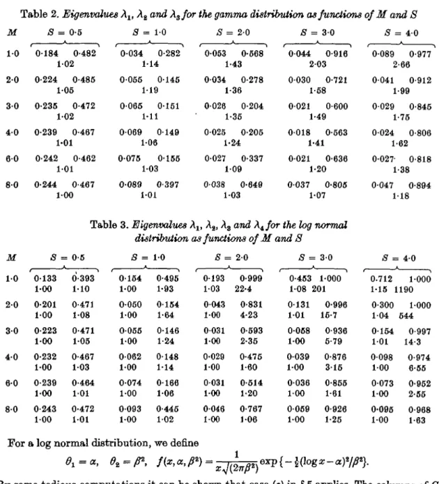
and all nontrivial eigenvalues of I—2 are negative, or one is negative and two are positive. For reasons of continuity the same alternative must hold for all a and A. I t turns out that the second alternative is true. Therefore, the nontrivial eigenvalues of 2 are 0 < Xx ^ Aa < 1 < A8. Table 2 gives Alf A2 and A8 for ji = 1,2,3,4,6,8, <rz and ;^a cells as for Table 1.

Table 2. Eigenvalues A1( A2 and Xzfor the gamma distribution as functions of M and S

M S = 0-5 5 = 1 - 0 5 = 2-0 5 = 3-0 5 = 4 0 1 0 2 0 3 0 4 0 6 0 8 0 0184 0-482 102 0-224 0-485 1-05 0-235 0-472 1-02 0-239 0-467 1-01 0-242 0-462 1-01 0-244 0-467 1-00 0-034 0-282 1-14 0055 0145 1-19 0-065 0-151 1-11 0069 0149 1-06 0-075 0-155 1-03 0089 0-397 1-01 0-053 0-568 1-43 0-034 0-278 1-36 0026 0-204 1-35 0025 0-205 1-24 0027 0-337 109 0038 0-649 1-03 0044 0 203 0030 0 1-58 0021 0 1-49 0018 0 1-41 0021 0 1-20 0037 0 1-07 •916 •721 •600 •563 •636 •805 f • 0-089 0-977 2-66 0041 0-912 1-99 0029 0-845 1-75 0-024 0-806 1-62 0-027- 0818 1-38 0-047 0-894 1-18

Table 3. Eigenvalues Alt A2, A3 and X^for the log normal distribution as functions of M and 8

M 5 = 0-5 5 = 1 - 0 5 = 2 - 0 5 = 3-0 5 = 40 1-0 0-133 0-393 0154 0-495 0193 0-999 0-453 1-000 0.712 1000 1-00 1-10 1-00 1-93 103 22-4 108 201 1-15 1190 2-0 0-201 0-471 0050 0154 0043 0-831 0131 0-996 0-300 1000 1-00 108 1-00 1-64 100 4-23 101 16-7 104 644 3-0 0-223 0-471 0055 0146 0031 0-593 0058 0-936 0154 0-997 1-00 105 1-00 1-24 1-00 2-35 1-00 5-79 101 14-3 4-0 0-232 0-467 0062 0-148 0-029 0-475 0039 0-876 0098 0-974 1-00 1-03 1-00 1-14 100 1-60 100 315 100 6-55 6-0 0-239 0-464 0074 0166 0031 0-514 0036 0-855 0073 0-952 1-00 101 1-00 106 1-00 1-20 100 1-61 100 2-55 8 0 0-243 0-472 0093 0-445 0046 0-767 0069 0-926 0-095 0-968 100 101 1-00 102 100 1-06 1-00 1-25 1-00 1-63

For a log normal distribution, we define

By some tedious computations it can be shown that case (c) in § 5 applies. The columns of G and M are independent and can be computed by the exponential and cumulative normal functions only. Of the four nontrivial eigenvalues of/ — £ two are positive and two are negative. Therefore, 2 has k — 5 eigenvalues 1, one eigenvalue 0, and four eigenvalues

0 < Aj < A2 < 1 < A8 < A4. Table 3 gives Ax, A2, A3 and A4, respectively.

In conclusion, we note that the x* test is still a standard technique during a preliminary analysis, whose users might sometimes be unaware of the underlying assumptions or unable to

Distribviion of the chi-squared test in nonstandard situations 121

get efficient estimates. The results should be seen as a warning against lining x2 tables with

k—lork — q—l degrees of freedom to reject the null hypothesis. For instance the 6 % rejection point based on 9 degrees of freedom is 16-9, while the approximate correct level corresponding to 16-9 in the log normal situation with M = 4 and S = 3 is about 11 %, and the correct rejection point for 5 % is 21.

This work was prepared with the support of the Swiss National Science Foundation and the U.S. Office of Naval Research.

REFERENCES

CHKBNOFS1, H. & LEHMANK, E. L. (1964). The use of the ma.ximnm likelihood estimates in %* tests for goodness of fit. Ann. Math. Statist. 25, 679-86.

CBAMEB, H. (1946). Mathematical Methods of Statistics. Princeton University Press. RA.O, C. R. (1973). Linear Statistical Inference, 2nd edition. New York: Wiley.

SUABLE, S. B. (1971). Linear Models. New York: Wiley.

WATSON, G. S. (1968). On ehi-square goodness-of-fit tests for continuous distributions. J. R. Statist. Soo. B 20, 44-61.