Adaptive stochastic control of linear systems with random parameters

WITH RANDOM PARAMETERS by Richard Tse-min Ku B.S., Massachusetts Institute (1970) S.M., Massachusetts Institute (1972)

E.E., Massachusetts Institute (1972)

of Technology

of Technology

of Technology

SUBMITTED IN PARTIAL FULFILLMENT OF THE REQUIREMENTS FOR THE

DEGREE OF

DOCTOR OF PHILOSOPHY at the

MASSACHUSETTS INSTITUTE OF TECHNOLOGY May, 1978

Signature of Author.../.

Department of Electrical Engineering and Computer Science, May 24, 1978

Certified by....r...,...r.-....r..-W - ---. N N-...

Thesis Supervisor Accepted by... .

WITH RANDOM PARAMETERS by

Richard Tse-min Ku

Submitted to the Department of Electrical Engineering and Computer Science on May 24, 1978 in partial fulfillment of the requirements for the Degree of Doctor of Philosophy.

ABSTRACT

In this thesis, we will investigate the adaptive stochastic control of linear dynamic systems with purely random parame-ters. Hence there is no posterior learning about the system parameters. The control law is non-dual; still it has the qualitative properties of an adaptive control law. In the perfect measurement case, the control law is modulated by the a priori level of uncertainty of the system parameters. The Certainty-Equivalence Principle does not hold.

This thesis shows that the optimal stochastic control of dynamic systems with uncertain parameters has certain limi-tations. For the linear-quadratic optimal control problem, it is shown that the infinite horizon solution does not exist if the parameter uncertainty exceeds a certain quantifiable threshold. By considering the discounted cost problem, we

have obtained some results on optimality versus stability for this class of stochastic control problems.

For the noisy sensor measurement case, we obtained the opti-mal fixed structure estimator-controller. The control law requires the solution of a coupled nonlinear two-point

boundary value problem. Computer simulations of the forward and backward difference equations provided some insight into the uncertainty threshold for the closed-loop system. Sto-chastic stability analysis further resulted in a sufficient condition for the mean square stability of the fixed structure dynamic compensator.

THESIS SUPERVISOR: Michael Athans

ACKNOWLEDGEMENTS

I want to thank my thesis supervisor Professor Michael Athans for his continued interest, guidance, and support for my re-search. Professor Athans always had a coherent sense of the on-going research direction and a tremendous insight of the analytical results. He has made a significant contribution to my doctoral education experience.

I would like to thank my thesis readers Professor Timothy Johnson and Dr. David Castanon. Professor Johnson provided many useful comments and in general helped to improve the

technical content of the thesis. Dr. Castanon helped out with some mathematical details in the thesis. I want to

thank my Graduate Counselor Professor Sanjoy Mitter for his concern for my graduate program. I like to thank Professors Edwin Kuh and Robert Pindyck of the Sloan School for their part in enriching my total doctoral research program.

I thank Professor Dimitri Bertsekas, Dr. Stanley Gershwin, and Demos Teneketzis for many valuable discussions on my thesis research. Technical comments contributed by Pro-fessors P. Varaiya, Y.C. Ho, J.C. Willems, and R. Gallager are acknowledged. I am deeply grateful to Jamie Eng for her timely assistance with the preparation of the thesis draft.

Thanks are due to the Technical Publications Department of The Analytic Sciences Corporation. Lillian Tibbetts typed superbly the thesis and James Powers created the art work. The computer work was done at the M.I.T. Information Pro-cessing Services on IBM 370/168.

This research was carried out at the M.I.T. Electronic Systems Laboratory with the partial support provided by

the National Science Foundation under Grant NSF/SOC-76-05827 and by the Air Force Office of Scientific Research under Grant AFOSR-77-3281.

To My Parents

Yun Chang Ku and Sau Chun Ku

TABLE OF CONTENTS ABSTRACT ACKNOWLEDGEMENT LIST OF FIGURES CHAPTER 1 CHAPTER 2 CHAPTER 3 INTRODUCTION

1.1 A Historical Survey of Adaptive Stochastic Control

1.2 Structure of the Thesis 1.3 Contributions of the Thesis

OPTIMAL STOCHASTIC CONTROL FOR THE PERFECT MEASUREMENT SYSTEM

2.1 Introduction

2.2 Problem Statement 2.3 Problem Solution

2.4 Asymptotic Behavior

2.5 Stochastic Stability Results 2.6 The Discounted Cost Problem 2.7 Control of Linear Systems With

Correlated Multiplicative and Additive Noises

2.8 Conclusions

OPTIMAL LINEAR ESTIMATION OF STOCHASTIC SYSTEMS WITH RANDOM PARAMETERS

3.1 Introduction

3.2 Problem Statement

3.3 Derivation of the Linear Minimum Variance Filter PAGE 2 3 8 10 10 17 20 24 24 25 27 35 52 60 70 73 75 75 77 79

-6-CHAPTER 4

CHAPTER 5

3.4 Linear Filter With Uncorrelated Parameters

3.5 Mutually Correlated Random Parameters 3.6 Conclusions

OPTIMUM CONTROL OF RANDOM PARAMETER SYSTEM WITH NOISY MEASUREMENTS

4.1 Introduction

4.2 Problem Statement

4.3 Optimum Solution of the Stochastic Control Problem

4.4 Formulation of the Deterministic Control Problem

4.5 Solution of the Deterministic Control Problem

4.6 Discussion of the Optimal Linear Controller

4.7 Optimum Stationary Linear Control 4.8 Stability of Stochastic Dynamical

Systems 4.9 Conclusions

ON LINEAR MULTIVARIABLE CONTROL SYSTEMS

5.1 Introduction

5.2 Optimal Control of Systems With Exact Measurements

5.3 Linear Multivariable Control for Systems With Scalar Random

Parameters

5.4 Optimal Control for Systems With Inexact Measurements 5.5 Conclusions PAGE 83 88 91 92 92 94 97 106 116 129 136 160 171 174 174 175 179 186 196

CHAPTER 6

APPENDIX A

APPENDIX B

REFERENCES

SUMMARY AND CONCLUSIONS

6.1 Summary of the Main Results 6.2 Conclusions

6.3 Suggestions for Future Research

DERIVATION OF THE OPTIMAL LINEAR CONTROL USING THE MATRIX MINIMUM PRINCIPLE

DERIVATION OF THE OPTIMAL LINEAR CONTROL USING DYNAMIC PROGRAMMING

BIOGRAPHICAL NOTE PAGE 197 197 200 202 205 211 223 231

-8-LIST OF FIGURES

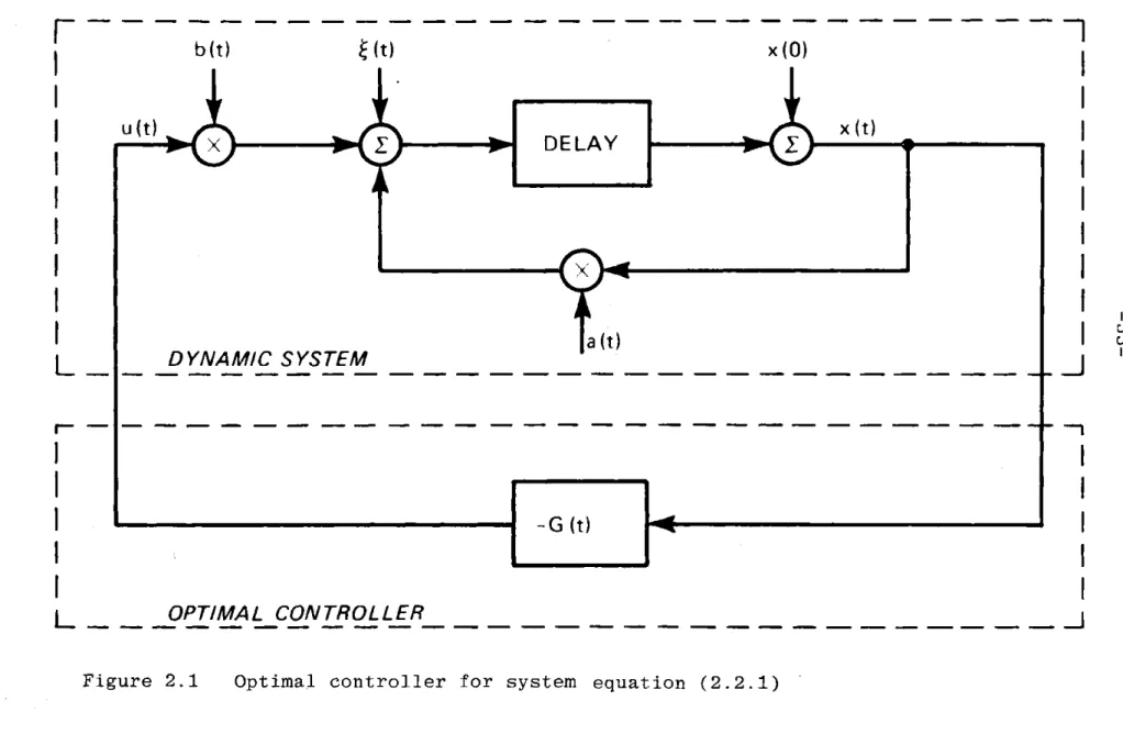
PAGE Figure 1.1 Stochastic control structure 14 Figure 2.1 Optimal controller for system

equation (2.2.1) 33

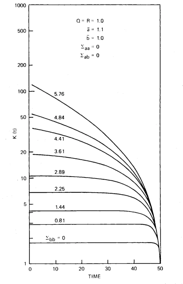
Figure 2.2 Solution of the Riccati-like equation

(2.4.1) for N=50 and known a(t)=i=1.1 37 Figure 2.3 Solution of the Riccati-like equation

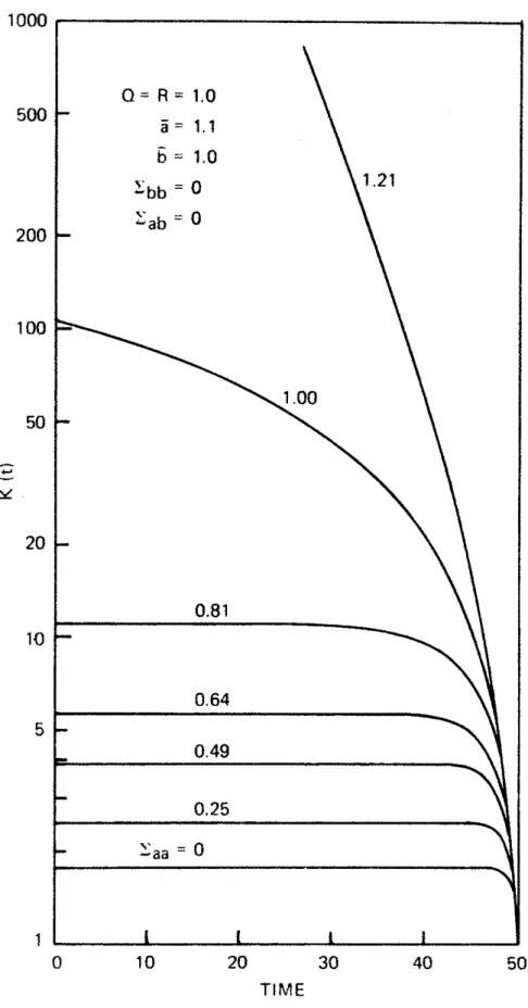
(2.4.1) for N=50 and known b(t)==1.0 38 Figure 2.4 Solution of the Riccati-like equation

(2.4.1) for N=50 when both a(t) and b(t)

are random 39

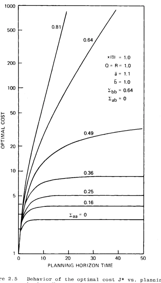
Figure 2.5 Behavior of the optimal cost J* vs

planning horizon N 41

Figure 2.6 Stability region defined by equation

(2.4.3) for system (2.2.1) 45

Figure 2.7 Stability regions defined by equation (2.4.3) for system (2.2.1) with known

a(t) =- 47

Figure 2.8 Stability region defined by equation

(2.4.3) for system (2.2.1) when b=0.0 50 Figure 2.9 Behavior of solution as a function of

threshold parameter m 66

Figure 2.10 Optimality and stability regions for

system equation (2.2.1) 69

Figure 3.1 Linear minimum variance unbiased esti-mator for stochastic system (3.2.1)

and (3.2.2) 85

Figure 4.1 Fixed structure linear controller and

estimator 108

Figure 4.2 Optimal fixed structure controller 119 Figure 4.3 Computed stability region for system given

PAGE Figure 4.4 Figure 4.5 Figure 4.6 Figure 4.7 Figure 4.8 Figure 4..9 Figure 4.10 Figure 4.11

Lower bound on the stability region defined by equation (4.7.26) for system given by equations (4.4.1) and (4.4.14)

Stability region defined by equation (4.7.27) for system given by equations (4.4.1) and (4.4.14)

Behavior of the states and costates given by equations (4.7.6) to (4.7.12) Behavior of the optimal control and filter gain sequences G(t) and H(t) Behavior of the divergent states and costates given by equations (4.7.6) to (4.7.12)

Solution of costate equation (4.7.18) for known a(t)=T=1.1 and b(t)=b=1.0 Solution of the costate equation

(4.7.23) for known a(t)=i=1.1

Solution of the costate equation (4.7.22) for known gain b(t)=b=1.0

146 147 148 149 151 152 153 154

CHAPTER 1 INTRODUCTION

1.1 A Historical Survey of Adaptive Stochastic Control

The theory of optimal closed-loop control of stochastic linear dynamic systems has progressed since the original con-tributions in [1], [2] . For discrete-time linear dynamic

systems with known system parameters and known additive gaussian noise statistics with quadratic cost, the optimum solution to the stochastic control problem is given by the Separation Theorem [3], [4]. These stochastic control-theoretic results have been reconciled with the statistical decision-theoretic

results given by the Certainty-Equivalence Principle for multi-stage decision processes [5], [6].

For linear dynamic systems with uncertain parameters or unknown noise statistics, there does not exist at present a general computationally feasible theory of optimum stochastic control. Bellman first presented a mathematical theory of

adaptive control processes in (7]. He introduced the concepts of "information pattern" and a control device that can "learn". Feldbaum expanded on the concept and algorithms of adaptive control in his four-part theory of dual control [8], so-called because the optimum controller must actively try to identify the unknown parameters as well as simultaneously control the system. He showed that in dual control systems, there may

-11-exist inherent conflict between applying the inputs for learn-ing and for effective control purposes. The dual control law is then to reflect the optimum interaction of caution and probing in the closed-loop control system. Feldbaum then distinguished between two kinds of loss, one due to the de-viation of the state and the other due to the nonoptimal learning control law [9].

The concepts of separation, certainty-equivalence, neutrality, and related dual control effects have been fur-ther clarified and discussed in [101-[16]. The present dual control action may influence future learning. In the

so-called neutral control systems described in [17], [18], learn-ing is independent of the control law. The neutral control law accounts for present uncertainty, but neglect the possi-bility that the present control action may influence future uncertainty resulting thus in a one-way separation.

Optimal solutions to the adaptive stochastic control of a class of linear dynamic systems with constant or time-varying unknown parameters can be obtained, in principle, using the stochastic dynamic programming method. The opti-mization algorithm is constructive and the solution is ob-tained by solving a recursive functional equation involving alternating minimizations and expectations, [8]., However, due to the "curse of dimensionality" the solution in general cannot be obtained analytically in closed form. The dynamic

programming algorithm encounters the problem of infinite dimensionality of the probability distribution function in the general case.

Since we cannot solve analytically the adaptive con-trol problem except for very special cases [19], [20], in practice we resort to approximation methods. The degradation

in performance of the suboptimal adaptive control law can be measured by comparing the average performance of the proposed

suboptimal control algorithm obtained from Monte Carlo simula-tions with the optimal but unattainable performance for the same control system in which the parameters are known with certainty.

There are two approaches to the approximation of the optimal adaptive control law. First, we may approximate the optimal solution to the adaptive stochastic control problem. This approach is taken in [7], [8], [11], [21-23]. The

second approach is to approximate the linear system as one with random parameters and derive the optimal adaptive stochastic control for the approximate control system. This can be done

by relaxing certain mathematical assumptions and information

structure of the optimal adaptive control law. In doing so, we may be able to obtain the suboptimal control law

analyti-cally. One such method is the enforced separation as in [241. Another is the open-loop feedback technique [25]-[30].

-13-Literature surveys and reviews of the state-of-the-art of adaptive control concepts and methods are found in

[311-[33]. An extensive bibliography on the theory and application of the various suboptimal adaptive estimation and control techniques is given in [34].

In this thesis, we will investigate a class of

stochastic optimal control problems with purely random (white) parameters whose mathematical solutions reflect some of the

aspects of adaptive stochastic control laws, Fig. 1.1.

The use of multiplicative white noise parameters explicitly tells the mathematics that the system dynamics are not known exactly and can vary in an unpredictable way. This is an

important class of problems because it represents a worst case design and analysis. The results provide some insights and help to evaluate whether the use of very sophisticated

identification and control algorithms may represent an "overkill".

Optimum control of linear systems with statistically independent random parameters is considered in [35]. For a constant linear system with multiplicative input noise, the effect of the random parameters was found to show the con-vergence of the feedback coefficients [2]. Necessary and sufficient conditions for a class of stationary linear system with random parameter to be controllable in mean-square sense was examined in [36]. Solution to the optimal stochastic

DISTURBANCES

CONTROLS

_MEASUREMENTS

SENSOR

Stochastic control structure

DYNAMIC

SYSTEM

CONTROLLER

-15-control problem with independent random parameter has been derived in [37], [38], and [391

The mathematical formulation of the stochastic con-trol problem with uncertain parameters forces the solution to be without any learning. In particular, we consider the

linear dynamical system

x(t+1) = A(t)x_(t) + B(t)u(t) + (t) (1.1.1)

t = 0,1,2,...,N-1

For simplicity we shall assume that the measurement is exact. The structure of the matrices A(t) and B(t) are known but the elements contain uncertain parameters. t(t) is the plant white noise (disturbance). The cost functional to be minimized is given by the scalar

N-1

J = E x'(N)Fx(N) +

Y

(1.1.2) where F, Q(-), and R(-) are at least positive semi-definite.

The uncertain parameters in A(-) and B(-) change

randomly with time. At each instant of time, "nature" selects the value of the system parameters from some a priori given distribution. The way "nature" selects the particular numeri-cal value of system parameters at each instant of time repre-sent a chance event in time. That is, the time-varying

tells the compensator that it cannot use the measurement data to improve the a prior mean or reduce the level of uncertainty of parameters anymore than the a prior variance. The optimal

solution cannot involve any learning about the system parameters. Although the mathematical formulation of the problem precludes identification, the solution of the optimal stochastic control problem in the sense of minimizing a cost functional shows the effects of parameter uncertainty in the performance of the control system. The control gain of an optimal stochas-tic system with randomly varying parameters will depend upon the unconditional means and covariances of the uncertain parameters. The Separation Theorem does not hold. Random-ness in the system parameters has strong influence on the gain of the control system, even in the absence of any learning.

The minimum value of the expected quadratic cost depends not only upon the means but also upon the variance of the randomly varying parameters. In the worst case sense, one has then an upper bound upon the performance deterioration of

the control system due to uncertain parameters. The difference between this worst case cost and the Separation Theorem cost

is the so-called value of model information for stochastic adaptive control problems.

This class of stochastic control problems is closely related to the state-dependent and control-dependent noise problem considered in continuous-time for perfect measurement

-17-[40] to [45] and in discrete-time for noisy measurement, [46] to [49]. The specific class of stochastic models given in Eq. 1.1.1 are also known as the multiplicative noise or random coefficient (multiplier) models. In [20] it is shown that if the only uncertainty parameter in Eq. 1.1.1 is in the matrix B then the nonlinear stochastic control system is

essentially a bilinear system. Hence the results for the class of adaptive control problems are readily applicable to the class of stochastic bilinear systems.

1.2 Structure of the Thesis

In this thesis, we will obtain the results almost entirely for the scalar systems. In the very simple first-order dynamical systems, we have no problem with system con-trollability or observability. The optimized stochastic control problem is well-posed and well-defined to give

existence and uniqueness results. The analytical results in the subsequent chapters for the scalar linear-quadratic-Gaussian systems must be true for

multivariable-nonlinear-non-Gaussian systems since the LQG problem is a special case of the more general formulation. The extension of these results to the multivariable case is conceptually straightforward, although notationally cumbersome.

The optimal stochastic control problem with perfect state measurement is considered in Chapter 2. The mathematical

formulation of the problem is given in Section 2.2. The solution to the "white noise parameters" optimization is ob-tained using the stochastic dynamic programming algorithm in Section 2.3. The important features of the control solution are discussed. In Section 2.4, we examine the steady-state solution of the optimal stochastic control problem. In parti-cular, we derive the inequality condition for the existence of a finite solution to the Riccati-like equation for infinite horizon problem. In Section 2.5, the stochastic optimization problem is treated as a stochastic stability problem. We give the necessary and sufficient conditions for the almost sure and mean square stability of the stochastic system under linear feedback. The concepts of optimality versus stability is further brought out in Section 2.6 when we consider the discounted cost problem. We extend the results in Section 2.3 to the case where the multiplicative noises are correlated with the additive noise in Section 2.7.

In Chapter 3, we treat the problem of optimum linear minimum variance estimation for the random parameter system. The estimation problem is stated in Section 3.1. The linear minimum variance filter is derived in Section 3.2. It is found that the parameter means and variances have to satisfy a necessary and sufficient condition for the asympotic vari-ance of the uncontrolled linear system to be finite (and this turns out to be sufficient to ensure stochastic stability as

-19-well). In Section 3.4, we discuss the case where the un-certain parameters are uncorrelated. In Section 3.5, the analysis is given to include mutually correlated randomly varying parameters.

In Chapter 4, we consider the closed-loop (feedback) control of randomly varying parameters system with noisy

measurements. The mathematical problem is formulated in Section 4.2. In Section 4.3 we examine the optimal solution to the control problem using stochastic dynamic programming.

In Section 4.4, we fix the structure of the class of dynamic compensates to be considered. We obtain the optimal param-eters (filter gains and control gains) first using the Matrix Minimum Principle and then dynamic programming algorithm. The important point is that we transformed the original stochastic control problem in Section 4.2 into a deterministic parameter optimization problem in Section 4.4. Section 4.5 shows that we have to solve a complex coupled nonlinear two-point boundary value problem in order to compute the optimal gains. We discuss the various aspects of the fixed structure estimate-controller

in Section 4.6. We consider the asymptotic behavior of the stochastic control law derived in Section 4.7. Numerical simulations of the stochastic equations provide the needed insights into the existence of steady-state control laws. Stochastic ability analysis analogous to that in Section 2.5 based on output feedback is given in Section 4.8. A sufficient

condition for the stochastic system to be mean-square stabi-lizable under feedback is presented.

In Chapter 5, we extend the results in Chapter 2 to a special class of linear multivariable systems. We give the mathematical formulation of the optimal stochastic control problem in Section 5.2. The solution via dynamic programming algorithm is given. In Section 5.3, we consider the optimal stochastic control of a multivariable linear system with a specific structure with respect to a quadratic performance

index. The system dynamics are described by a linear vector difference equation with white, possibly mutually correlated, scalar random parameters. In Section 5.4 we summarize the results on the adaptive stochastic control of linear multi-variable systems with imperfect measurements.

We summarize the results on the optimum stochastic control of linear dynamic systems with purely random param-eters in Section 6.1. We make conclusions about optimality

and stochastic stability in Section 6.2. We discuss the existence, finiteness, and convergence of the derived opti-mal control law. In Section 6.3, we recommend the

direc-tions for future research in this area.

1.3 Contributions of the Thesis

The optimal stochastic control results for the exact state measurements problem have been known for some time in

-21-[37]. _{However, their potential importance and their}

im-plications in adaptive control has not yet been fully

realized. _{This thesis reports on the research of the optimal} stochastic control of white noise parameter systems. The objective is to gain deeper insights and clearer understand-ing of the issues and philosophy of the adaptive control. Even in the absence of learning, the degree of dynamic un-certainty (as quantified by the variances of the

multi-plicative white noise parameters) influences both the optimal control gains and the optimal value of the performance index.

In this thesis research we shall analyze stochastic systems with white parameters as a worst case to provide a systematic analysis and design approach to adaptive stochas-tic control. _{We derive the upper bound on the average cost} for the exact measurement and the noise-corrupted measure-ment cases. _{We analyze the dual nature of stochastic control} for systems with uncertain parameters in a most transparent mathematical framework. _{The mathematical formulation} pre-cludes any learning about the parameters, however.

We derive the necessary and sufficient condition for the optimal control law for the perfect measurement case. We then derive the necessary and sufficient condition for the stochastic stability in the almost sure and mean-square sense for the class of stochastic systems under consideration. The Uncertainty Threshold Principle then says there exists a

threshold of dynamic uncertainty, if exceeded then optimal strategies cannot exist. We have derived the optimality condition for the discounted cost problem. The problem provides an interesting and important case study of opti-mality versus stability problem in stochastic control theory. We were also able to extend the analysis on control to the

case where the multiplicative noises are correlated with additive noises.

In deterministic linear quadratic control problem the duality principle holds, that is, the linear stochastic estimation problem is related through duality to the optimal deterministic control problem. The dual of the control prob-lem with the pair (C',B') is the estimation probprob-lem pair (B,C). For linear discrete-time systems, duality principle says that the various matrices that occur in the optimal regulator

problem and the optimal state reconstruction problem are related and have symmetry property, [50]. We show that this duality property does not hold for the optimal regula-tor and optimum linear minimum variance estimation problems for the class of adaptive stochastic control problems. In particular, the stability condition for the asymptotic be-havior of the optimum linear minimum variance filter problem cannot be obtained by "dualizing" the stability condition

-23-We have obtained the linear minimum variance un-biased filter with deterministic control input. Results are generalized to the case where all the random parameters may be correlated. _{The necessary and sufficient condition for} the asymptotic stability of the state second moment turns out to be only a sufficient condition for the stochastic stability of the fixed structure overall closed-loop system.

For the noisy sensor measurement case, we derived the fixed structure dynamic compensator using dynamic pro-gramming algorithm. We determined the average cost expression (in a worst case sense). _{The use of direct output feedback} is shown to give only a sufficient condition for the mean-square stability for the overall control system.

CHAPTER 2

OPTIMAL STOCHASTIC CONTROL FOR THE PERFECT MEASUREMENT SYSTEM

2.1 Introduction

In this chapter, the optimal control problem.for purely random parameters will be formulated and solved for the perfect observation case. We present the mathematical model of a class of stochastic linear systems in Section 2.2 and give the technical assumptions about the statistical laws for the random processes. The optimal stochastic control problem is then formulated assuming perfect measurements.

In Section 2.3, we give the solution to the optimal control problem via dynamic programming. In Section 2.4, we examine

the stability properties of a stationary system. The Un-certainty Threshold Principle is given in Theorem 2.1. We examine the stochastic stability of a linear system under linear feedback in Section 2.5. In Section 2.6, we discuss the discounted cost problem and give a modified threshold for the particular cost functional chosen. We discuss some important new issues in stochastic controllability and sta-bility. In Section 2.7, we extend the results of Sections 2.2 and 2.4 to linear systems where the random parameters and the additive noise are correlated.

-25-2.2 Problem Statement

In this section, we will state the problem. Con-sider a first-order stochastic linear dynamical system with state x(t) and control u(t) described by the difference equation

x(t+1) = a(t)x(t) + b(t)u(t) + (t) (2.2.1)

t = 0,1,2,...,N-1

x(0) given.

We assume that the additive noise F(t) driving the system dynamics is a zero-mean Gaussian white noise with known variance

E{((t) (T)} = E(t)6(t,T) (2.2.2)

We assume that the purely random parameters a(t) and b(t)

are Gaussian and white (uncorrelated in time) with known means a(t) and b(t), and covariances Zaa(t) and Ebb(t), respectively and cross-covariance given by Eab(t). More precisely, we

assume that

E{a(t)} = a(t) , E{b(t)} = b(t) Vt (2.2.3)

and

E a(t) - a(t)) (a(T - a(T) = aa(t)6(t,T)(2.2.4)

E{(b(t) - b(t)) (b(T) - b(T))} = Ebb(t)6(tT) (2.2.5)

where 6(t,T) is the Kronecker delta and

2

aat)Ebb(t) -Z2(t) 20(2.2.7) since the correlation coefficient

|pI

It is assumed that the additive white noise E(t) is statistically independent of the random parameters a(t) and b(t). The case where a(t), b(t), and E(t) are correlated is discussed later in Section 2.7.

For the stochastic control problem it is very

important to specify the information available for control. In this chapter, we assume that the state x(t) can be mea-sured exactly. Hence we assume that x(O) is given.

We assume that the admissible controls are real-valued and of state feedback type u(t) = y(x(t),t). The control can only depend on the given a priori information and measurements up to time t. The control u(t) at time t can only influence the state x(T) at T -t+1 and not before. This is the important notion of causal inputs - past and present output values do not depend on future input values.

The optimal control problem is to determine the control law u(t)=y(x(t),t)(t=0,1,...,N-1) such that the expected value of a quadratic cost functional is minimized. The quadratic cost functional is the standard regulator type.

J()

(.;),F2(N)

-1

J(C)= E Fx (N) +Y x2(t)Q(t) + u (t)R(t)

a(-),b(-), t= O

-27-The expectation is taken with respect to the probability distribution of the underlying random variables a(t), b(t), and t(t).

Based upon the application of the Bellman's Principle of Optimality and functional equations, dynamic programming is used to solve the optimal control problem formulated in Eqs. (2.2.1) and (2.2.8).

2.3 Problem Solution

The solution to the optimal control problem given in Eqs. (2.2.1) and (2.2.8) can be obtained by applying the standard dynamic programming method. The cost-to-go at the final time is given by

2

V(x(N),N) = Fx (N) (2.3.1)

By the Principle of Optimality

V(x(N-1),N-1) = min E Q(N-1)x2 (N-1) + R(N-1)u2(N-1) u(N-1) a(N-1),

b(N-1),

(NN--+ V(x(N),N)IXN-(

SMin[Q(N-1) _{+ F(a}2

_(N-1)+E

x2(N-1) u(N-1)a

+ R(N-1) + F(b2(N-1)+Ebb(N--1))1 u2_(N-1)

+ 2F(a(N-1)b(N-1) + Zab(N-1))x(N-1)u(N-1)

since E(N-1) is independent of u(N-1) and x(N-1) and the random parameters a(N-1) and b(N-1).

We minimize the algebraic expression in Eq. (2.3.2) by taking the derivative with respect to u(N-1) and setting

it to zero, we obtain as a result

u * (N-i)

_{u N1}

₂

_ab

_x(N-1)

(2. 3. 3)

(b (N-1) + Ebb(N-1) )F + R(N-1)

Substituting this optimal control at N-1 into cost Eq. (2.3.2) the optimum cost-to-go becomes

V(x(N-1),N-1) = x2(N-1)K(N-1) + F;E (N-1) (2.3.4) where K(N-1) = F( E aa(N-1) + a2(N-1)) +Q(N-1) - G2(N-1) [R(N-1) + F(b2(N-1) +Ebb(N-1))1 (2.3.5) F [a(N-1)(N-1) + Eab(N-1)]

G(N-i)

-2(2.3.6)

We note that the optimum cost-to-go at time N-1 is of the same form as Eq. (2.3.1). The second term is due to the additive noise driving the system. The first term in-cludes the cost of control and implicitly the added cost due to the randomness of the parameters a(N-1) and b(N-1).

-29-At time N-2, the cost-to-go is given by the equa-tion V(x(N-2),N-2) = min E Q(N-2)x2(N-2) + R(N-2)u (N-2) u(N-2) + V(x(N-1),N-1)IX>N-2 Smin E Q(N-2)x2(N-2) + R(N-2)u2(N-2) u(N-2) + K(N-1)x2(N-1)JXN-2 ₊ FB-n(N-1) (2.3.7) This expression for the cost-to-go is identical to that in Eq. (2.3.2) except for the time indexes. Therefore, the optimal control u (N-2) is given by

u (N-2) = -K(N-1)(a(N-2)b(N-2) _{+ E} (N-2)) -2) ab (b (N-2) + Ebb(N-2))K(N-1) + R(N-2) x(N-2) (2.3.8) and the optimal cost-to-go is given by

*

2

By induction on t, we obtain the solution to the

stochastic state regulator problem. Given the linear stochastic (2.3.9)

system Eq. (2.2.1) and the cost functional Eq. (2.2.8), where u(t) is not constrained, the optimal feedback control

at each instant of time is given by a linear transformation of the state, * u (t) = -G(t) x(t) (2.3.11) K(t+l)(Eb(t) + a(t)b(t)) G(t) = -2 R(t) + (Ebb(t) +b (t))K(t+1) (2.3.12)

and K(t) is the solution of the Riccati-like equation

=

-2

K(t) (a (t) + E a(t))K(t+1) + Q(t)

- G2(t) R(t) +K(t+l)(Ebb(t) +E2(t))] (2.3.13)

satisfying the boundary condition

K(N) =

F

The state of the optimal system is then the solution of the linear difference equation

x(t+1) = a(t) - b(t) K(t+1)(E (t) + a(t)b(t))

1

The optimal control given by Eq. (2.3.11) is a random variable since x(t) is a random variable. It is linear in the completely measurable state. The uncertainty where

-31-in the parameters a(t) and b(t) -31-introduces equivalent state and control weightings, E (t)K(t+1) and Ebb(t)K(t+1),

respectively in a very natural way into the control problem. In order for the extremal control to be the unique optimal control, we need to show that the second partial derivative of T with respect to u,

R(t) + (Ebb(t) + b2 (t))K(t+1) > 0 (2.3.16)

The solution to the Riccati-like Eq. (2.3.13) is non-negative definite. This can be seen from the fact that for any x.

x K(t) = min E x2Q(t) un X ) + R(t) u

+ ( a(t )x + b(t )u) 2K( t+1),

K(N) = F > 0 (2.3.17)

Since F,Q(t) >0 and R(t) >0, the expression within the bracket is non-negative. Since the minimization over u preserves

non-2

negativity, it follows that x2K(t) 0 for all x. Hence, K(t) is non-negative definite. Since R(t) is positive definite, we conclude that [R(t) +(Ebb(t) +b (t))K(t+1)] >0.

The Riccati-like Eq. (2.3.13) is a first-order non-linear time-varying ordinary difference equation, the solution K(t) exists and is unique. The external control given by

Eq. (2.3.11) is, therefore, the unique optimal control. The optimal cost-to-go is obtained by substituting the expression for the optimal control Eqs. (2.3.11) and

* 2 N-1

J (x(t),t) = K(t)x (t) + I K(T+1) H (T) (2.3.18)

T=t

If the optimal control u(t) t0 for all states then K(t) > 0 for all Oct <N. This follows from the fact if u(t)t0, then the cost T must be positive. We shall say that an optimal

*

control exists, when J is defined for all x(t) and t.

Figure 2.1 shows the structure of the optimal feed-back system. Since the optimal control is u(t) =-G(t)x(t), the state x(t) is multiplied by the linear gain G(t) to gen-erate the control. The optimal feedback system is, thus,

linear and time-varying in the finite horizon problem. This will be the case even if the system is stationary and the cost

functional is time-invariant. Note that the optimal control given by Eqs. (2.3.11) to (2.3.13) is modulated by the

co-variances of the purely random (white) parameters. The optimal controller is cautious when the parameter b(t) is uncertain. The gain G(t) is smaller in magnitude, ceteris paribus, than

the linear-quadratic gain. The controller is more vigorous when the parameter a(t) is uncertain, since the controller must be more active to regulate the system. The gain G(t) are larger in magnitude, ceteris paribus, with larger vari-ance E (t).

Since the gain G(t) is a function of K(t), the solution K(t) to the Riccati-like Eq. (2.3.13) governs the behavior of the optimal feedback system. The Eq. (2.3.13)

Ut)x M) X DELAY x a (t)

L

LOPTIMA L CONTROL LER

is nonlinear and, in general, we cannot obtain closed-form solutions. We shall discuss in the next section the solution K(t) to Eq. (2.3.13) as N-+o- to obtain a steady-state con-troller for the stationary system and cost functional with constant weightings.

We remark that the optimal control law given by Eqs. (2.3.11) to (2.3.13) is not the Certainty-Equivalent control, since the control gain depends on the parameter variances. The Certainty-Equivalent control law is

u .(t) = - b(t)K(t+1)a(t) x(t) (2.3.19) b (t)K(t+1) + R(t) where

-2-2

2

-2

This can be obtained from Eqs. (2.3.11) to (2.3.13) by setting arbitrarily E aa(t) = Ebb(t) = Eab (t) = 0. The

Certainty-Equivalence control law does not account for the uncertainty in the system parameters.

The optimal stochastic control is without posterior learning. The parameters a(t) and b(t) cannot be identified, because by assumption they are white. Nature/chance picks the parameters and the controller must adapt to the structural change. This is a worst-case control system design, as com-pared to assuming the parameters are unknown but constant or

-35-slowly time-varying. However, the assumption of purely random parameters is unrealistic from a physical point of view. The assumption that the parameters are unknown but constant leads to the well-known dual control problem whose exact solution cannot be easily computed analytically. The white parameter assumption leads to a very simple stochastic

control law Eq. (2.3.11) that can be easily implemented. Economists, and in particular Chow [38] have argued that in economic systems, treatment of unknown parameters as being purely random is desirable to obtain the inherent caution

in the control especially when b(t) is not known accurately. In [32], Athans and Varaiya have argued that the control of systems with white parameters represents a worst-case situa-tion in which the ratio

K(OJZ

/0, Z

f

0, E

# 0)

aa Ebb ab > 1 (2.3.21)

K(O|E =0, Z =0, Z =0)

aa bb ab

provides a measure of the deterioration in performance due to the unknown parameters, which can provide a guide as to whether sophisticated parameter estimation and adaptive control algorithms are warranted.

2.4 Asymptotic Behavior

We assume in this section that the stochastic linear system given by Eq. (2.2.1) has wide-sense stationary statistics.

The state and control weightings Q(t) and R(t) are assumed to be constant.

The Riccati-like Eq. (2.3.13) is then given by

2 2

K(t) =

Q

aa

-2

(ba+Ebb)K(t+l) + R

K(N) = 0

Since the nonlinear difference Eq. (2.4.1) has con-stant parameters, one may well think that it will attain a steady-state solution "backward in time" as it certainly does for the ordinary linear-quadratic problem with known param-eters, so' that one can then calculate the infinite horizon (constant) gain. This is, however, not the case for Eq. (2.4.1).

Figures 2.2, 2.3, and 2.4 show the numerical solu-tion of Eq. (2.4.1) for N =50 for different values of means and covariances of the parameters. Note the logarithmic scale used. A close examination of Eq. (2.4.1) shows what can happen to the solution K(t) of the Riccati equation.

Consider then Eq. (2.4.1) and assume that K(t+1) is "large". Then the "backward in time" evolution of K(t) is given approximately by

K(t) z K(t+1)m (2.4.2)

where the threshold parameter m is given by -2

(E +a b)

m = E + a ab -2(2.4.3)

aa

E

5

-37-Q= R = 1.0 5 = 1.1 b = 1.0 -aa ab=0 - 5.76 - 4.84 4.41 - 3.61 2.89 2.25 0.81 b bb0 20 TIME

Figure 2.2 Solution of the Riccati-like equation (2.4.1) for N=50 and known a(t)=a=1.1

1000 500

1-200

100

50

20

10

5

1000

500

200

100

50

20

10

5

Figure 2.3 Solution of the Riccati-like equation (2.4.1) for N=50 and known b(t)=b=1.0

Q= R = 1.0 a = 1.1 b = 1.0

~bb

1

1000 500 -0.81 200 Q R = 1.0 a= 1.1 100 b=1.0 bb = 0.64 0.64 ab0

50

Figure 2.4 Solution of the Riccati-like equation (2.4.1) for N=50 when both a(t) and b(t) are random

or

-2 -2 2

Z + Z b + E a - Z - 2E ab

M-aa bb aa bb -2 ab ab (2.4.4)

Ebb + b

Clearly, from Eq. (2.4.2) K(t) will undergo expo-nential growth "backward in time" if

m > 1 (2.4.5)

From the expression in Eq. (2.4.3) or (2.4.4) one can see that there are certain combinations of the parameter means and covariances that will yield the inequality condition in

Eq. (2.4.5). Hence, we can immediately arrive at the con-clusion that in the case of optimal stochastic control with purely random (white) parameters, a well-behaved solution to

the infinite horizon problem may not exist.

A different insight can be provided by examining

the dependence of the optimal cost upon the planning horizon. Figure 2.5 shows the behavior of the optimal cost versus time N. Note that if the threshold parameter m >1 then the optimal

cost grows exponentially,

*2 mN

J (N)~x2(0)e , m>1 (2.4.6)

Otherwise (m <1) the optimal cost remains bounded and finite. Now, suppose that Eq. (2.4.1) has a steady-state solution given by

i

2 -- 2

K= K( 9 + Z ) + - (Zab 2ab)(2.4.7)

-41-1000 500- 0.81 0.64 x (0) = 1.0 200 _{0= 0- R= 1.0} 5 = 1. 1 b = 1.0 100 bb = 0.64 lab =0 50 0.49 20 10 -0.36 0.25 5 0.16 2aa= 0 0 10 20 30 40 50

PLANNING HORIZON TIME

Figure 2.5 _{Behavior of the optimal cost J* vs. planning} horizon N

Note that K must be positive definite. The solution to the quadratic equation is then given by

it

Q(Ebb+b2

- (R( E aa+a2) -

QZbb+b2

L

)-Eabb+

The limiting solution

i

-- 2 (Z +ab)2 -2 ab +-2 ) aa Z -2 Z bbb (2.4.9) or m<i (2.4.1

We state the following result. Theorem 2.1

The unique positive solution to the infinite horizon problem given by Eqs. (2.2.1)-(2.2.7) exists if and only if m <1.

Proof: (==) we rewrite the Riccati-like Eq. (2.3.13), re-versing the time index; as

0)

[(E

21

1bbb

[-2

-43-Since the third term is non-negative definite (R >0),

K(t+1) >

Q

>

2

Q

m

It follows immediately that if m >1, then K(t) diverges as t +CO.

Since. the third term is monotone increasing in K(t), it follows that K(t) is monotone increasing for K(0)=

Q.

M(t) = K(t) - RK(t)

-2 + K(t) Ebb+ b

(2.4.13)

Note that M(t) is also monotone for positive R. Thus there exists an a >0 such that

-2 Z +b

M-(t) _{K(t) + R} -1 (2.4.14)

from which we have that M(t) is uniformly bounded in K(t), that is,

M(t) < a , ct>0 (2.4.15)

F2

1

Q

L

ab

4

so that K(t) is bounded as t+oo because m <1.

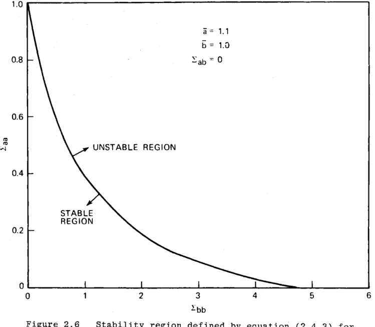
Since there is a sharp dividing line, quantified by the means and covariances of the random parameters, between the cases that the optimal stochastic control exists or does not exist for the infinite horizon case (see Fig. 2.6) it is obvious that there is a fundamental limitation to optimal

infinite time quadratic control problem. We call this

phenomenon, the Uncertainty Threshold Principle. This result has several implications in engineering and socioeconomic systems, since it points out there is a clear quantifiable boundary between our ability of making optimal decisions or not (in the sense that the optimal cost is bounded) as a

function of the parameter modeling uncertainty.

Katayama [51] has pointed out this instability problem when b(t) is random in a multivariable system. For

continuous-time systems the existence of solutions has been investigated by Bismut [45], but only for finite horizon

ii 1.1

1.3

0.6

0

Figure 2.6 _{Stability region defined by equation (2.4.3) for} system (2.2.1)

problems. In related problems involving control-dependent noise, Kleinman [41] assumed the existence of a solution.

In the case of known parameters (Eaa Ebb= ab = 0) Eq. (2.4.4) yields m=0. This is the reason why there is no problem with the stationary solution for standard linear quadratic problem.

In the case where a(t)= a (E

_aa

_ab

-2

M=bb (2.4.17)

E b

_Ebb

-2

so that as long as a is less than or approximately equal to one, then m < 1 and there is no convergence problem for the

solution K(t) to the Riccati-like Eq. (2.4.1), (see Fig. 2.7). This may possibly explain Kleinman's results [41] on control-dependent noise problems and their application for pilot

models controlling stable aircraft. This is also the same stability condition derived by Katayama for random gains [51].

In the case where b(t) =b (Ebb= 0 =Eab), Eq. (2.4.4)

yields m =E . This implies that independent of the average

aa

values of a and b, as long as the variance E of the "time constant" a of the system exceeds unity, then one is in

trouble for long horizon planning problems, even for systems that are stable on the average (lai <1). This result seems to state that when the standard deviation of the parameter

4.0 3.0 a = 1.2 UNSTABLE 2.0 ST ABL E 1.0

0

Figure 2.7 Stability regions defined by equation (2.4.3) for system (2.2.1) with known a(t)=a

a(t) is greater than unity, then the system is statistically mean-square unstable, and under these conditions, one cannot stabilize the system.. This provides a tie with the literature on stochastic stability with state-dependent noises ([52], [53]).

From Eq. (2.4.3), it is evident that a non-zero parameter correlation (Zab > 0) always reduces the value of

m, and hence it helps prevent (up to a point) the divergence of K(t). From a modeling viewpoint, this implies that a careful modeling of the relationship of the joint statistics

in the coefficients that multiply the state variables and those that multiply the control variables can only help.

Suppose that the threshold parameter m c 1 so that a steady-state

Z

G = lim G(t) = A -2 (2.4.18)

N-*oo R+K(Ebb+b

)

is well-defined. Since the gain G(t) is constant, the re-sulting optimal system will be linear and constant; from engineering point of view, such an optimal controller would be very simple to construct for stationary systems.

Next, suppose that b =0, so that the system (2.2.1) is "most uncontrollable on the average". Note that Gt0 and u(t) t 0 provided that the correlation Zab j 0. This means heuristically that the random time constant system is

controllable in a stochastic sense; the nonzero covariance 2ab means that a(t) and b(t) "swing together" and this implies that we can still control a system which is "most uncontrol-lable on the average". _{This observation seems to suggest a} new concept of "stochastic controllability".

Note that in the case b=0, the uncertainty threshold parameter m is given by

2E 22

aa bb ab -2

M =b+ _{a (2.4.19)}

2

_bb

In view of the fact (2.2.7), this "stochastic controllability" is possible only for systems that are stable on the average ( I _{<1), otherwise m >1 (see Fig. 2.8).}

Suppose now that the threshold parameter m > 1, so

that the optimal cost given by Eq. (2.3.14) grows exponentially with the time horizon N. The control gain remains, however, a well-defined quantity, and is given by the constant value

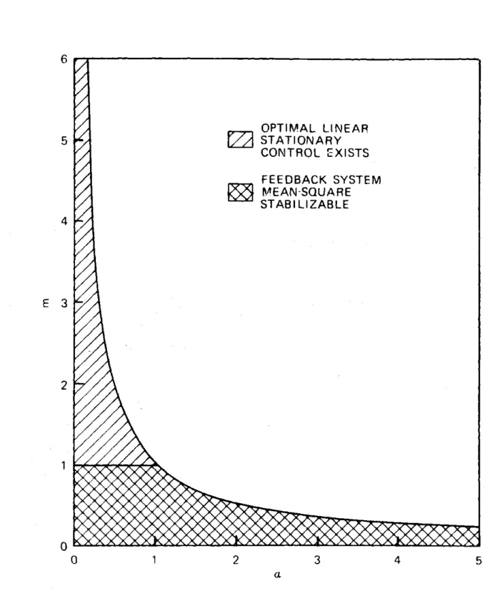
2b+ab

G 2ab(2.4.20)

2 +b b

bb

which is obtained by letting K(t+1)-+oo in Eq. (2.3.13). One could argue that there is an optimal limiting gain in the sense that one is still trying to do his best so as to mini-mize the rate of the exponential growth of the optimal cost

1.0

0.8

-0.2

0

0

0.2

0.4

0.6

0.8

1.0

Figure 2.8 Stability region defined by equation (2.4.3) for system (2.2.1) when b=0.0

To see further the implication of this philosophy one can substitute the gain G in the system dynamics Eq. (2.2.1) and obtain the stochastic control system

x(t+1) = (a(t) - b(t) G) x(t) _(2.4.21)

Under the assumption that x(t) can be measured exactly the mean x(t) =E{x(t)} will propagate (in an open-loop sense) as

x(t+1) = (a - b G) x(t), x(O) = x(O) (2.4.22)

The state error covariance (t) A E x(t) -x(t)

xx

can then be shown to propagate according to

(t+1) =mZ(t)+ xx xx ()

aa

~-2

where m is the threshold parameter given by Eq. (2.4.13). It is clear that if m >1 in Eq. (2.4.24) then the open-loop propagation of the variance of the state Z (t) is

xx

unstable. _{Essentially, this says that although the} steady-state control is well-defined by a constant gain Eq. (2.4.20), and the closed-loop system of Eq. (2.4.21) can be implemented,

the variability of the state as measured by its variance "blows up" as t becomes large.

A sufficient condition that will ensure that the inequality (2.4.10) will be met is

-2

E'aa + a < 1 (2.4.25)

This condition is both a necessary and sufficient condition for the asymptotic variance of the uncontrolled linear system

x(t+1) = a(t) x(t) (2.4.26)

to be finite, and thus turns out to be sufficient to ensure that an optimal control exists as well.

2.5 Stochastic Stability Results

We want to now analyze the optimal control problem posed in Section 2.2 from an alternative point of view and arrive at exactly the same conclusions. The approach treats the stochastic control problem as essentially a mathematical problem, that is, stochastic difference equation and we will consider the stochastic stability of such system under feed-back. Asymptotic stability of linear stochastic systems

with random coefficients have been considered in t52] to [57]. Consider the first-order linear dynamical system

x(t+1) = a(t) x(t) + b(t) u(t) (2.5.1)

One can include additive white noise driving the system dynamics, but the stability result is unchanged from the

whether or not the system Eq. (2.5.1) is stabilizable under feedback when a(t) and b(t) are assumed to be random coeffi-cients.

Let

u(t) = g(t) x(t) (2.5.2)

Thus the closed-loop system will propagate according to the stochastic equation.

x(t+1) = a(t) + g(t) b(t)Ax(t) A C(t) (2.5.3)

If a(t) and b(t) are uncorrelated in time, one can calculate the ratio

2

E{x (t+1)} =E 2 2 2 A

2 Efc(1)}E{c (2)}. . .E{c

(t)}

The value of S(t) is a measure of how the second moment of the state propagates in time. The larger the value of S(t), the more variable the state is. In particular if

lim S(t) + (2.5.5)

t -ao

the system (2.5.3) is unstable in the mean square sense. The value of S(t) will be influenced in part by the value of the feedback gain g(t) in Eq. (2.5.2). So one can seek the value of g(t) which will minimize the ratio S(t) in Eq. (2.5.4).

The product S(t) is minimized if each element of the product

is minimized by g(t). Since

E{c2 (t)} = Efa2(t)} + g2(t) Etb (t)} + 2g(t) Eta(t)b(t)} (2.5.7) therefore, the best value of g(t) is obtained by algebraic minimization which yields

Eab + a b

g

g (t)

bb

2

Hence the minimum value of E{c (t)} is given by

2*

2

E{c (t)} =

E{a(t)

+

-

b

m

bb

where m is the undiscounted threshold parameter given by Eq. (2.4.3).

It follows that

*

t

S(t) = m (2.5.10)

and hence that

lim S (t) < 00 if m < 1. (2.5.11)

We state the results in the following theorem. Theorem 2.2

The stochastic system in Eq. (2.5.1) is stabilizable by linear feedback in a mean-square sense if and only if the

uncertainty threshold parameter m, defined by Eq. (2.4.3) is less than unity.

* We note that the minimum variance gain g in

Eq. (2.5.9) is the same as G in Eq. (2.4.20) where we

con-cluded that the limiting control gain is a constant and the feedback system can be implemented. The feedback system may or may not be stabilizable under feedback depending on

whether or not the threshold parameter m < 1 is satisfied.

The stochastic stability analysis resulted in an optimal gain g(t) given by Eq. (2.5.8) which is identical to Eq. (2.4.20). It yields the sufficient condition for optimal

control to exist. Since we are considering mean-square stability, we could have obtained the same gain by setting R =0 in the cost functional Eq. (2.2.8); and then Eq. (2.4.18) becomes Eq. (2.5.8). The stochastic stability condition is thus independent of the numerical solution K.

Following Kozin [58], we consider now the "almost sure stability" analysis (sample path stability) of the stochastic linear system Eq. (2.5.1) under feedback Eq.

(2.5.2).

Definition 2.5.1. The equilibrium solution x(t) =0 of the system

x(t+1) = (a(t) + b(t) g(t)) x(t)

= c(t) x(t) (2.5.12)

where

x(0) = x₀ is a random variable

(2.5.13) lim P sup sup x(t~w) > =

0

6+-%-0

for any given e > 0 and 6(e,O) > 0.

For discrete-time systems, an equivalent condition is given in [59].

Definition 2.5.2. _{The equilibrium solution x(t) =0 of the} system Eq. (2.5.12) is almost surely stable if for s > 0

lim P sup x(t) > = 0 (2.5.14)

x₀

1+O

Accordingly, Konstantinov in [591 proved the following: Theorem 2.3

The solution x(t) = 0 of the system (2.5.12) is almost surely stable for t20 if there exists a function V(t,x) EDL (domain of definition) which for t > 0 satisfies the conditions

(i) V(t,x) is continuous at x=0 and V(t,0)=0 (ii) inf V(t,x) > a(6) > 0 for any 6>0

jxj>6

(iii) L[V(t,x)] : 0 in some neighborhood of x =0. A suitable Lyapunov function to use is

V(t,x) = x2(t) (2.5.15)

Then condition (iii) in Theorem 2.3 says that

E{V(t+1,x) - V(t,x)1 < 0 (2.5.16) and using Eq. (2.5.12)

-2

2

2

a + 2a b g(t) + b g t) 1 (2.5.17)

We now show that for Ia+_bg(t)I<1, then almost every sample sequence {x(t)} would approach zero. Following [54], we have

Theorem 2.4

The equilibrium solution of Eq. (2.5.12) is almost surely stable if ja+bgl < 1

Proof: We must show that lim P sup

6+*0 _Ix01<6

1.im P sup

6+*0

|x01<6

sup

Ix(tw)I

tL0

sup

t20

= 0 _(2.5.18)

Ix(tw) I

lim P sup sup cp(t,0) 6+0

[x

I1,X₀I > E (2.5.19)

where $(t,O) is the solution of the difference equation

$(t+1,0) = c(t) (t,0) _(2.5.20)

Hence, Eq. (2.5.19) becomes lim P sup $(tt,0)I >

4

6+0 t>0 lim

P

_$(t,0)

sup

K$(t,0)1

>

4

Therefore, the first term in Eq. (2.5.21) is given by but,

lim P sup

6-+o

I$(t,0)I >

4

=

lim

P

sup

$(t,0)I

nc

n-*oo 0 t: T w)

= no)w:

sup

$(t,0)J

>

ne(]

n=1

OstsT(w)

=0

since

Ia

For ergodic process in the parameters,

1rn -(t,w) = E{4(t,w)}

t -co0t

(2.5.23)

(2.5.24)

Given $ > _{0, there exists then a random time T (W)}

such that $(t,w) - E{$(t,w)} C for all t > T (w). Since

a.s.

for all t > T (w) and -t

$(tw) < t(ct +

)