Object Location using Edge-Bounded Planar Surfaces from Sparse Range Data

Publisher’s version / Version de l'éditeur:

CCGEI 2003 Canadian Conference on Electrical and Computer Engineering,

TF289, 2003

READ THESE TERMS AND CONDITIONS CAREFULLY BEFORE USING THIS WEBSITE.

https://nrc-publications.canada.ca/eng/copyright

Vous avez des questions? Nous pouvons vous aider. Pour communiquer directement avec un auteur, consultez la première page de la revue dans laquelle son article a été publié afin de trouver ses coordonnées. Si vous n’arrivez pas à les repérer, communiquez avec nous à PublicationsArchive-ArchivesPublications@nrc-cnrc.gc.ca.

Questions? Contact the NRC Publications Archive team at

PublicationsArchive-ArchivesPublications@nrc-cnrc.gc.ca. If you wish to email the authors directly, please see the first page of the publication for their contact information.

NRC Publications Archive

Archives des publications du CNRC

This publication could be one of several versions: author’s original, accepted manuscript or the publisher’s version. / La version de cette publication peut être l’une des suivantes : la version prépublication de l’auteur, la version acceptée du manuscrit ou la version de l’éditeur.

Access and use of this website and the material on it are subject to the Terms and Conditions set forth at

Object Location using Edge-Bounded Planar Surfaces from Sparse

Range Data

MacKinnon, David; Blais, François; Aitken, C.

https://publications-cnrc.canada.ca/fra/droits

L’accès à ce site Web et l’utilisation de son contenu sont assujettis aux conditions présentées dans le site LISEZ CES CONDITIONS ATTENTIVEMENT AVANT D’UTILISER CE SITE WEB.

NRC Publications Record / Notice d'Archives des publications de CNRC:

https://nrc-publications.canada.ca/eng/view/object/?id=30480481-9da4-41c6-9279-5f6b9091d0bb https://publications-cnrc.canada.ca/fra/voir/objet/?id=30480481-9da4-41c6-9279-5f6b9091d0bb

National Research Council Canada Institute for Information Technology Conseil national de recherches Canada Institut de technologie de l'information

.

Object Location using Edge-Bounded Planar

Surfaces from Sparse Range Data *

MacKinnon, D., Blais, F., Aitken, C.

May 2003

* published in IEEE Canada, CCGEI 2003 Canadian Conference on Electrical and Computer Engineering May 4-7, 2003, Canada, TF289, pp. 1-6. NRC 45831.

Copyright 2003 by

National Research Council of Canada

Permission is granted to quote short excerpts and to reproduce figures and tables from this report, provided that the source of such material is fully acknowledged.

O

L

E

-

P

S

S

R

D

David K. MacKinnon

Carleton University

david.mackinnon@nrc.ca

Francois Blais

National Research Council

of Canada

francois.blais@nrc.ca

Victor C. Aitken

Carleton University

vaitken@sce.carleton.ca

Abstract

This paper describes a method for performing object location by applying edge detection techniques to sparse range data generated using a laser range scanner (LRS) developed by the National Research Council (NRC) of Canada [2]. Range data consisted of closed-loop line scans resulting from Lissajous scanning patterns that are currently under investigation by the NRC [4].

Current investigations in object detection and tracking using Lissajous scanning patterns have demonstrated the ability of the system to track objects in real-time using a simple planar representation [6]. In this study we adapt traditional edge detection techniques to convert range data obtained using a Lissajous scanning pattern into sparse edge maps. We represent an object as a single planar surface by combining the original range data with object boundaries defined by the edge map.

Data collected from typical LRS systems was used to develop a noise model for use with a simulated model of the LRS system [7]. We then compared two edge enhancement methods to examine the effect of window size on edge sensitivity under simulated noise conditions. Edge maps were generated to approximate simple planar surfaces that were used to represent a single object in both simulated and real environments. Results show that this method is successful in locating a simple object in a static environment.

Keywords: laser range data, edge detection, object

location

1. INTRODUCTION

The National Research Council of Canada (NRC) developed a laser range scanner (LRS) to perform object detection and tracking at ranges between 0.5-10 metres using triangulation and up-to 2-kilometres using time-of-flight [2]. The system can obtain range and intensity information using either a raster scan pattern

or a Lissajous scan pattern. In real-time tracking mode the system uses one or more Lissajous scanning patterns to obtain sparse range or intensity maps [4]

.

We are currently investigating methods to locate and track objects by performing edge detection using sparse range data. An accurate model was recently developed for Matlab so much of this work was performed using simulated data. This model has been calibrated for the triangulation mode of operation between 1.0-metre to 10.0-metres range [7].

2. EDGE DETECTION

We define an edge detection algorithm as a computational method by which raw image data is converted into an image consisting of single-pixel-width edge data. This involves noise filtering, edge enhancement and edge localization [8, pp.69-71]. Our goal is to detect edges that represent images boundaries so we restrict ourselves to the detection of step edges.

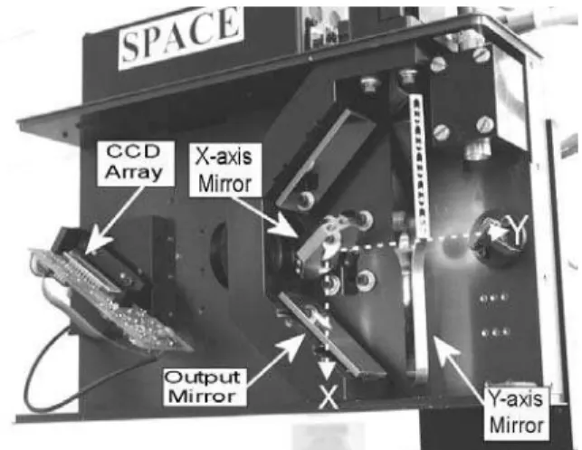
Figure 1. Typical LRS unit used at NRC

CCECE 2003 – CCGEI 2003, Montréal. May/mai 2003 0-7803-7781-8/03/$17.00 © 2003 IEEE

-001-

In this study we work in UVP space rather than the traditional Cartesian XYZ space. UVP space consists of horizontal (U) and vertical (V) angular measurements and a range (P) measurement. Working directly in the raw UVP space allows us to avoid the errors inherent in converting UVP to other measurement spaces when calibrating the data; UVP errors are uncorrelated which is not the case in the XYZ domain. Furthermore, avoiding calibration enable us to obtain real-time performances at low cost. In Figure 1 we see the galvanometer-controlled x-axis and y-axis mirrors. A/D converters read the galvanometers position and generate the U and V readings as 16-bit signed integers. Also visible is the CCD array that is sampled by a peak detector to generate a 16-bit signed integer peak (P) reading that corresponds to 1/64 of a CCD pixel. The peak reading represents the directed distance from the LRS unit to a surface in the environment.

Figure 2. Simulation of a flat box with 0.5-metre edge height 1-0.5-metre from the LSR unit

Surfaces that are flat in Cartesian space appear as smoothly curved surfaces in UVP space. Moreover we are using data obtained using a nonlinear scanning pattern so significant range changes can appear as artefacts of the movement of the laser. The edge detection algorithm must be able to distinguish step edges from curvatures induced by the scanning pattern. Figure 2 shows the results of a simulated Lissajous scan of a box.

2.1 Noise Filtering

UVP data was expected to display both random Gaussian and spike noise. Spike noise would consist of erroneous peak measurements, non-detected peak values and saturated peak signals. Non-detected peak values are represented as zeroes while saturated peak signals are represented as negative numbers.

Data was collected from a LRS unit of Figure 1 at 1, 3, 5, 7 and 9-metres. At each range 10 repetitions of a 256-point (3,4) Lissajous scan was performed.

All peak values equal to zero were removed and marked as Zero Spike readings. At each point the sample standard deviation si was calculated. If si was

greater than 100 then outliers were iteratively removed and marked as Non-Zero Spike readings until the new sample standard deviation was less than or equal to 100 (approximately 1.5 CCD pixel). The worst-case variance of the remaining data was calculated and represented as the worst-case SNR. The spike rates were represented as a frequency of occurrence. Table 1 summarizes the results.

Table 1. Observed noise in LRS data

Measure Calib Wavelength 820-nm Standard error Zero-Spike Non-Zero Spike 7.059×10-5 0.0078 0.0000

Four common noise filters were evaluated to determine which would return a signal that best matched the ideal pre-noise signal. These filters were the Gaussian filter [9, pp59-60], local averaging filter [9, pp57-58], local median filter [9, pp65-68] and iterated local median filter [10]. The iterated median filter was restricted to a window size of 3-elements.

A 1024-element array was generated to represent the ideal (pre-noise) results of a Lissajous scan. The first 512 elements were assigned a value of 25000 representing surface 2-metres from the scanner. The remaining 512 elements were assigned a value of 2500+24 to represent a step edge. Gaussian and spike noise were added to the ideal signal using the observed noise levels and resulting signal was passed through the noise filter.

Filter error was calculated as the sum of the absolute deviations between the ideal and filtered signal normalized to the base peak value of 25000. The average normalized absolute deviation (AAD) was then calculated for 100 repetitions. In the case of averaging, Gaussian and Median filters the optimum window size were selected as the best compromise between AAD improvement and minimizing computation time.

Table 2. Optimal noise filtering results. Filter Type Window Size AAD (N=100)

Gaussian Averaging Iterated Median Median 11 9 3 11 25.73 ± 0.339 12.95 ± 0.411 0.29 ± 0.079 0.04 ± 0.000 The results of comparing noise filters can be seen in Table 2. There was a significant difference among the filter types based on a univariate analysis of variance

(uANOVA) at p=0.000. Based on a Scheffée multiple-comparison test, Erosion and Median filters were significantly better than Gaussian or Averaging but not significantly different than each other [15, pp.141-142]. We use the Median filter in the remainder of this study.

2.2 Edge Enhancement

Noise filtration is not expected to remove all noise but simply to reduce noise effects to a tolerable level. The ability of the product-of-difference (PoD) edge enhancement method to filter noise is known to improve with window size while sensitivity to edges decreases [9, pp103-105]. We compare the PoD filter to the traditional 3-element first derivative filter (Der) filter as an example of a small-window filter [11, pp143-145]. Previous experiments with the PoD filter in combination with 3-element median filter indicated that a PoD window size of 11 elements could be tolerated without affecting the real-time performance of a LRS unit [13].

Figure 3. PoD response to step and ramp edges.

PoD values were thresholded based on trial-and-error experimentation to a minimum value of 60 to minimize noise effects. Edge detection of Peak values, like many range metrics, is affected by scale variability [12] so the PoD value was normalized by the maximum PoD value. The normalized PoD value was further thresholded to a minimum value of 0.3 based on trial-and-error experimentation.

Derivative edge enhancement values were thresholded based on trial-and-error experimentation to a minimum value of 14 before being normalized by the maximum Der value. The normalized Der values were thresholded to a minimum value of 0.2 based on trial-and-error experimentation.

An examination of typical normalised PoD and Der output shows that peaks resulting from step and steep ramp inputs closely approximate a triangle. Peaks resulting from shallower slopes are more curved and

have a wider base. The base to peak-height ratio was calculated for each peak and an upper limit was determined based on observation. For the 11-element PoD edge enhancement method the upper limit was 27 while the limit for the 3-element Der edge enhancement method was 3.5. Figure 3 shows the results of PoD edge enhancement of both step and ramp edges.

Figure 4. Average number of edges detected by PoD and Der methods as a function of range between 0.5-m and 10.0-m (N=10)

2.3 Edge Localization

The results of edge enhancement were filtered using a custom peak detector. The filter removed all but the non-zero local maxima and utilized a 5-element window. If two or more consecutive non-zero values were detected then the non-zero element corresponding to the largest peak value (i.e. closest to the LRS unit) was selected and the others are replaced with zero elements. This guarantees that each edge is represented by a single non-zero element.

2.4 Edge Detector Performance

The ability of the each edge detection method to detect the boundaries of an object within the 0.5-metre to 10.0-metre range was examined by varying the range of a surface against background 1000-metres from the scanner. In Figure 4 it can be seen that the PoD method detects the correct number of edges within the required range. The Der method detected significant false edges at longer ranges.

Edge detector sensitivity with regard to step edges was examined at 1 and 10-metres. A simple box object was simulated and scanned using a 1024-element (3:4) Lissajous scan pattern. Figure 5 shows that although the Der method was more sensitive to edge height it detected edges at short range when the edge height was actually zero.

Figure 5. Average PoD and Der method sensitivity at short (1.0-m) and medium (10.0-m) range (N=10)

Edge slope sensitivity was examined using a ramped transition between a surface at 1.0-metres and a surface at 5.0-metres. An increase in the width of the transition region was used to approximate a decrease in edge slope. Region width was measured as a fraction of the total scan width. Figure 6 shows that the PoD method produced fewer spurious edges as edge slope increased and eventually ceased to detect edges at steep slopes. Ideally only 5 edges should be detected. We see that the Der filter is more susceptible to the effects of edge slope.

Figure 6. Average number of detected edges for PoD and Der method as a function of edge slope (N=10)

Edge detector performance can be tuned by adjusting the peak base-to-peak width ratio as well as the edge enhancement threshold. This can be used to improve performance where noise levels differ from those used in this simulation. In practice an operator would increase the edge sensitivity by reducing the edge enhancement threshold but this increases the effect of noise. Increasing the peak base-to-peak width ratio would result in detecting ramp edges with

shallower slopes. However this would increase the rate of false edges due to UVP surface curvature artefacts.

3. OBJECT LOCATION

We calculate the location of the edge centroid as the average U and V value based on the edges detected. We assume that there is only one object visible in the scan and that the edges mark the object boundaries. We also assume that the object is closer to the scanner than the background.

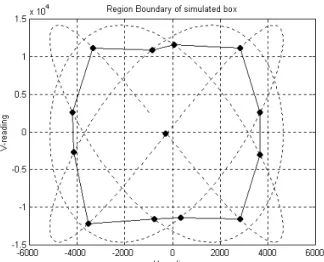
Figure 7. Region boundary of simulated box object in the UV plane.

Figure 8. Planar surface representation of a simulated box object.

For each edge we extract a pair of UVP points and select the UVP point with the smallest peak value as being within the object boundaries. This peak value is selected as the peak associated with the edge point.

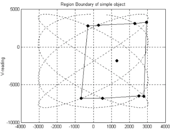
Figure 9. Edges detected of a simple planar object

Figure 11. Angle view of simple object

We decouple the edge points from the Lissajous scan by calculating the angle of a line segment from the edge centroid to each edge. The edges are then sorted based on the rotation angle to define the object boundary in the UV plane. In UVP space flat surfaces appear curved so a flat surface cannot be represented accurately as a single planar surface. We instead represent the surface as a series of non-overlapping triangular surface elements.

Figure 12. Front view of simple object

A (4:3) Lissajous scan of a simple planar object was performed using a prototype laser scanner. Figure 9 shows the detected edges as black dots and the estimated region boundaries as solid lines. Figure 10 shows the same object in UVP-space with edges and the edges centroid marked as black dots. Two views of the original object can be seen in Figures 11 and 12.

Figure 10. Planar surface representation of a simple object

Figure 7 shows the detected edges of a simple box surface 4.9-metres from the scanner on a surface 5.0-metres from the scanner. The black dots connected by lines represent detected edges and the black dot in the centre represents the edge centroid. Figure 8 shows the same object in UVP-space. The black dots represent detected edges and the edge centroid. The range of centroid is the average range (peak value) of all detected edges. The planar representation of the object can be seen as a series of triangular planar elements.

4. CONCLUSION

A simulation of a laser range scanner developed by the National Research Council of Canada was calibrated to display similar noise characteristics to those observed in the real scanner. An 11-element

median filter was found to provide the best recovery of the original signal when corrupted by the observed noise model.

Large and small window edge enhancement methods were compared to determine which provides the best performance with non-linear sparse range scans in UVP space. All edge enhancement data was thresholded and normalized, and the normalized data was thresholded to minimize noise. Peaks with base-to-height ratio larger than a threshold value were eliminated so that only step and steep ramp edges would be selected. Edges were reduced to single pixel-width using a custom peak detector method.

The large-window edge enhancement routine was found to perform better than the small-window routine using step edges within the 0.5 to 10-metre range. The large-window routine was also better able to handle ramp edges of varying edge slopes.

Edges detected using the large-window were used to define region boundaries. These region boundaries were then used to construct planar elements to represent simple surfaces. Surfaces of simple objects were successfully located under both simulated and actual conditions.

Acknowledgements

The authors would like to thank the Natural Science and Engineering Research Council of Canada (NSERC) for providing financial support for this research. The authors would also like to thank Michel Picard of the NRC for his assistance in data collection.

References

[1] Livingstone, F.R., King, L., Beraldin, J.-A., Rioux. M. “Development of a Real-time Laser Scanning System for Object Recognition, Inspection, and Robot Control” in Telemanipulator Technology

and Space Robotics SPIE, Vol.2057, pp.454-461,

1993. (NRC-35063)

[2] Beraldin, J.-A., Blais, F., Rioux, M., Cournoyer, L., Laurin,D., and MacLean, S. “Short and medium range 3D sensing for space applications.” in SPIE Proceedings of Visual Information

Processing VI (Aerosense '97) Vol.3074,

pp.29-46, Orlando, FL. 21-25 April 2000. (NRC 40170) [3] Beraldin, J.-A., Blais, F., Rioux, M., Cournoyer,

L., Laurin, D., and MacLean, S.G. “Eye-safe digital 3D sensing for space applications.” Optical

Engineering SOIE, Vol.39, No.1, pp.196-211,

January 2000. (NRC 43585)

[4] Blais, F., Beraldin, J.-A., Cournoyer, L., El-Hakim, S.F., Picard M., Domey, J., Rioux, M., Christie, I., Serafini, R., Pepper G., MacLean S.G., and Laurin D.. “Target Tracking Object Pose Estimation, and Effect of the Sun on the NRC 3-D Laser Tracker.” in Proceedings of iSAIRAS-2001 Montreal, Quebec, June 2001. (NRC 44876) [5] Blais, F., Beraldin, J.-A., Cournoyer, L.,

El-Hakim, S.F., Domey, J., and Rioux, M. “The NRC 3D Laser Tracking System: IIT’s Contribution to International Space Station Project.” in

Proceedings of the 2001 Workshop of Italy-Canada on 3D Digital Imaging and Modeling Application of: Heritage, Industry, Medicine, & Land Padova, Italy, 3-4 April 2001. (NRC 44181)

[6] Blais, F., Beraldin, J.-A., El-Hakim, S.F., and Cournoyer, L. “Real-time Geometrical Tracking and Pose Estimation using Laser Triangulation and Photogrammetry.” in Proceedings of the Third

International Conference on 3-D Digital Imaging and Modeling IEEE, pp.205-212, Quebec City,

Quebec, 28 May-1 June 2001. (NRC 44180). [7] MacKinnon, David K., Blais, Francois, Aitken,

Victor C. “Modeling an Auto-synchronizing Laser Range Scanner”, to be presented at 2003 American

Control Conference, 4 – 6 June 2003.

[8] Trucco, E., and Verri, A. Introductory Techniques

for 3D Computer Vision. Prentice-Hall, 1998.

[9] Ritter, G.X. and Wilson, J.N. Handbook of

Computer Vision Algorithms in Image Algebra, 2nd edition. CRC Press, 2000.

[10] Burian, A. and Kuosmanen, P., “Tuning the smoothness of the recursive median filter”, IEEE

Transactions on Signal Processing, Vol.50, Iss.7,

pp.1631-1639, 2002.

[11] Jain, R., Kasturi, R. and Schunck, B.G., Machine

Vision. McGraw-Hill, Inc., 1995.

[12] Oliver, C.J., Blacknell, D. and White, R.G., “Optimum edge detection in SAR” IEE

Proceedings on Radar, Sonar and Navigation,

Vol.143, Iss.1, pp.31-40, 1996.

[13] MacKinnon, David K. “Real-time Edge Detection using the Random Access Scanner” internal presentation to Visual Information Technology group at the National Research Council of Canada, August 2001

[14] Pratt, W.K., Digital Image Processing, 3rd

edition. John Wiley and Sons, 2001.

[15] Keppel, Geoffrey, Saufley, William H., Jr.,

Introduction to Design and Analysis: A Student’s Handbook. W.H. Freeman and Company, New

York, 1980.