HAL Id: hal-01823058
https://hal.archives-ouvertes.fr/hal-01823058
Submitted on 25 Jun 2018
HAL is a multi-disciplinary open access archive for the deposit and dissemination of sci-entific research documents, whether they are pub-lished or not. The documents may come from teaching and research institutions in France or abroad, or from public or private research centers.
L’archive ouverte pluridisciplinaire HAL, est destinée au dépôt et à la diffusion de documents scientifiques de niveau recherche, publiés ou non, émanant des établissements d’enseignement et de recherche français ou étrangers, des laboratoires publics ou privés.
Corruption determinants in developing and transition
economies: Insights from a multi-level analysis
Joel Cariolle
To cite this version:
Joel Cariolle. Corruption determinants in developing and transition economies: Insights from a multi-level analysis. 2018. �hal-01823058�
fondation pour les études et recherches sur le développement international
LA FERDI EST UNE FOND
ATION REC ONNUE D ’UTILITÉ PUBLIQUE . ELLE ME T EN ŒUVRE A VEC L ’IDDRI L ’INITIA TIVE POUR LE DÉ VEL OPPEMENT E
T LA GOUVERNANCE MONDIALE (IDGM).
ELLE C
OORDONNE LE LABEX IDGM+ QUI L
’ASSOCIE A U CERDI E T À L ’IDDRI. CE TTE PUBLIC ATION A BÉNÉFICIÉ D ’UNE AIDE DE L ’É TA T FR AN Ç AIS GÉRÉE P AR L ’ANR A U TITRE DU PR OGR A MME «INVESTISSEMENT S D ’A VENIR» POR
TANT LA RÉFÉRENCE «ANR-10-LABX
-14-01».
Abstract
This paper re-examines the contribution of five major corruption determinants emphasized by the literature, through an empirical analysis based on a hierarchical modelling of firm-level corruption data. Exploiting a baseline sample of 34,358 bribe reports of firms from 71 developing and transition countries, I use a three-level estimation framework to study the contribution of the economic and human development levels, the size of governments, trade openness, and democracy. Multi-level estimations stress that the negative effect of income per capita on bribery is found to be mostly driven by improvement in human capital, more particularly by the decline in fertility rates. They also allow the reconciling of some contrasting findings of the literature on other corruption determinants, but point that the contribution of corruption determinants is context-dependent.
JEL codes: D73; D02; D22; P48; O57
Keywords : Corruption ; Bribery ; Firm ; multi-level model ; hierarchical model. Acknowledgment
I am grateful to Simone Bertoli, Olivier Cadot, Jean-Louis Combes, Vianney Dequiedt, Sébastien Desbureaux, Bernard Gauthier, Michaël Goujon, Patrick Guillaumont, Jean-Pierre Laffargue, Frédéric Lesné, and Alexander Sarris for useful discussions and comments. I also thank
Corruption determinants in
developing and transition
economies:
Insights from a multi-level
analysis
Joël Cariolle
Joël Cariolle, Research officer at FERDI. Email: [email protected],
229
June 2018Dev
elopment Po
lic
ie
s
Wo
rkin
g Paper
“Sur quoi la fondera-t-il l’économie du monde qu’il veut
gouverner? Sera-ce sur le caprice de chaque particulier? Quelle
confusion! Sera-ce sur la justice? Il l’ignore.”
1. Introduction
Corruption is a complex and multi-faceted phenomenon, hard to define, to measure and to tackle. For decades, it has received wide attention from sociologists, political scientists, legal scholars, and economists, and significant resources have been devoted by governments, the civil society, and International Institutions to measure it and to combat it. While corruption is still pervasive in many developing countries, progresses have been made regarding its measurement – as more direct survey-based measures of corruption experiences progressively replaced indirect expert-based corruption perception indicators in cross-country analyses – and policies aimed at controlling it – shifting from a public sector-centred perspective to broader multi-stakeholders anti-corruption strategies. Academically, socio-economic analyses of corruption determinants still abut on a range of biases caused by the secretive and fuzzy nature of corruption transactions (Lesne, 2013).
From a public-sector perspective, corruption is often depicted as an individually-driven phenomenon, resulting from a cost-benefit analysis ensuing from tension between public agents’ public responsibilities and the perspective of personal gains (Banfield, 1975). From a business perspective, corruption transactions are either seen as a constraint upon firm’s operations, or an investment made to obtain undue preferential treatments from the public sector and to yield private payoffs (Banfield, 1975; Martin et al, 2007; Transparency International, 2009). In this last setting, corruption may be compatible with corporate objectives, and may result from a tension between an organization’s pecuniary objectives and the legal, cultural and social norms of ethics and integrity that prevail in a social group (Rose-Ackerman, 2007; Martin et al, 2007). And from a societal perspective, corrupt transactions are also driven by holistic factors that go beyond individual and organizational motives. Shared norms of ethics, trust, and coordination that prevail in a given society or a social group may indeed make corrupt individual decisions related to each other (Andvig, 2006; Blundo et al, 2006).
In a micro-level empirical analysis of country-level corruption determinants, this interdependence of corruption decisions at different levels of a society – location, sector, country, or region – may result in estimation biases (Moulton, 1990). This so-called “intra-class correlation” problem can, however, be addressed through multi-level modelling of corruption data (Martin et al, 2007). This paper is a review of the contribution of five major corruption determinants emphasized by the literature – the economic and human development levels, the alleged oversize of the government, trade openness, and democracy – in light of a multi-level analysis applied to a sample of 34,358 bribe reports of firms from 71 developing countries. This paper therefore extends efforts undertaken by a vast literature to identify key corruption determinants (Klitgaard, 1988; Rose-Ackerman, 1996; Bardhan, 1997; Tanzi, 1998; La Porta et al., 1999; Treisman, 2000, 2007; Lambsdorff, 2002, 2005; Mauro, 2004; Svensson, 2005; Dreher et al., 2007), by exploiting a large database on firm-level experiences of corruption, and by applying a multi-level empirical framework that accounts for the context of corrupt transactions.
In line with previous empirical research, multi-level estimates confirm that economic development, measured by income per capita, significantly and negatively contributes to bribe prevalence. However, this negative effect of income per capita is found to be mostly driven by improvement in human capital, more particularly by the decline in fertility rates. In fact, raising the fertility rate by one child per women is found to almost double bribe prevalence in the baseline sample, which is equivalent to the effect of a 10% decline in GDP per capita on bribe payments. Regarding education, higher school attendance is associated with smaller bribe payments but higher corruption incidence. This contrasting evidence on the relationship between human capital and corruption is found to be partly mediated by the public spending channel. One explanation is that more educated people require more public spending, and hence larger rents in the economy, but they also induce a better monitoring of public action (Eicher et al., 2009). In this regard, public intervention is found to have a positive effect on bribery through public spending, but a negative one through taxation. This result suggests that a larger government size may be both associated with larger rents and better institutions. Larger state intervention is also found to mediate part of the positive effect of trade openness on bribery, but this positive effect also lies in countries’ inclination to natural openness. Last, results reveal a negative effect of political rights and press freedom on corruption, but also show that young democracies may experience higher corruption levels because of the larger scope for private transactions. All in all, the significance of random coefficients across estimations, and the sensitivity of coefficient estimates to their inclusion, suggest that the contributions of key corruption determinants emphasized in this study are nevertheless highly context-dependent.
The next section reviews business and socio-economic studies that highlight the contextual origin of corrupt transactions. The third section sets a multi-level model of corruption prevalence that takes into account the contexts of corruption occurrence. In the fourth section, a three-level empirical analysis of five key corruption determinants is undertaken and commented in light of the literature’s findings. The fifth section concludes.
2. The contextual origin of corrupt transactions
Economic literature generally views corruption from the demand side of corrupt transactions (Martin et al., 2007). Defined by the World Bank as the abuse of public office for personal gains, corruption is often confined to a consequence of state interventions aimed at correcting market failures (Shleifer & Vishny, 1993; Banerjee, 1997; Acemoglu & Verdier, 2000). Standard economic approaches therefore depict corruption as an individually-driven phenomenon, resulting from public agents’ discretionary power over public resources allocation and a lack of accountability in the public sector (Klitgaard, 1988). In this setting, corrupt transactions result from a cost-benefit trade-off, and arise from the tension between public agent’s private interests and the general interest (Banfield, 1975).
On the other hand, business studies view corruption from the supply side of corrupt transactions. They note that firms’ decisions to engage in corruption may fully match their objective of profit maximization (Banfield, 1975), so that corrupt transactions result from the prevalence of profitability objectives over the organizational and societal value of ethics. This point is also highlighted by social science studies that stress how holistic norms of honesty, integrity and trust in a society strongly frame individual corrupt decisions (Blundo et al., 2006).
In socio-economic studies, particular attention has been paid to the effects of social capital and its manifestations – such social norms of honesty, ethics, and trust – on corrupt exchanges (Lambsdorff & Frank, 2011; Graeff, 2005). In this regard, the importance of reciprocity as a key principle that guides corrupt deals has been investigated (Lambsdorff and Frank, 2011; Graeff, 2005). By specifying how corrupt agents should behave in particular situations, corruption norms structure corrupt exchanges, especially when agents and clients do not know each other, and so, may not trust each other.
When such social norms of corruption do not fully operate, the level of trust between individuals can ensure the reciprocity in corrupt exchanges (Graeff, 2005). A few economic analyses have addressed the structuring role of interpersonal trust by emphasizing that frequent and prolonged interactions between corrupt actors allow them to reinforce reciprocity in corrupt deals (Andvig & Moene, 1990). Corruption may therefore be encouraged through various types of network membership – such as kinship or friendship, age, ethnic group, gender, social/religious cast, or religion – so that corruption may be persistent even in societies with broad civic and ethical norms.
However, other studies consider that trust and social norms of honesty may be self-reinforcing features of a society. Uslaner (2005) points out that trust – when defined as a “value expressing the belief that others are part of your moral community” (Uslaner, 2005, p.76) – discourages corrupt behaviours by enhancing the coexistence of citizens and contributing to the respect of laws, values of ethics, and morality. In line with this argument, Fisman and Miguel’s (2007, 2008) analysis of UN diplomats’ inclination to break the law suggests that corruption prevalence in a given country depends on people’s “sentiments towards their own country’s laws” (Firsman & Miguel, 2008, p.100). Thus, according to these studies, the frontier between trust and adherence to “corrupt” or “ethical” social norms is porous.
Therefore, while studies insist on various cross-country features that give public agents’ incentives to engage in corruption, others reframe corrupt transactions within their context of occurrence. In the next sub-section, I explain why a multi-level empirical framework is particularly suited for the contextual analysis of cross-country determinants of corruption prevalence.
3. A multi-level empirical framework for the analysis of corruption prevalence
3.1. A multi-level estimation framework
Multi-level or hierarchical models depict a hierarchical system in which units of observations are nested within groups, and groups are nested within higher-level groups (Hox, 2010). These models, widely applied to human capital analysis (Hitt et al., 2007), exploit the hierarchical structure of micro datasets to relax the hypothesis of independence of observations within different levels of the data. The relevance of these models for the analysis of corrupt deals is that, because of shared social norms of ethics, trust, and coordination modes prevailing in a given society or a social group, corrupt individual decisions may be correlated with each other. Applying a multi-level framework for the analysis of bribery determinants seems therefore particularly suitable, by allowing a contextualization of economic agents’ decisions within the different groups to which they belong.
A multi-level corruption model is useful when there is one dependent corruption variable measured at the lowest level, e.g. the firm or individual experience or perception of corruption offences, explained by various corruption determinants measured at all levels of the data. The three-level “country-sector-firm” model adopted in this paper is a hierarchical system of equations where the dependent variable, the firm k’s experience of bribery (Yi,j,k), is explained by firms’
characteristics (Hi,j,k) (e.g. large or small firm), the sector j’s characteristics (Zi,j) (e.g. sector’s tax
pressure) and the country i’s characteristics (Xi) (e.g. government’s public spending). In this
multi-level estimation framework, we would regress:
, , , , . , . , , . , , , , (1)
With α a country-sector intercept, α , α and are country-sector regression coefficients, and e, , a usual zero-mean and constant-variance error term. Therefore, contrary to usual single-level models, a three-single-level model assumes that each sector, in each country, is characterized by a different intercept and different slope coefficients. In other words, while the single-level model assumes that observations are independent across levels of the data, multi-level models relax this hypothesis.
By setting random coefficients in the model, this three-level model posits that, in our example, the relationship between the firm’s size and bribery ( , ), the relationship between the sector-level tax pressure and firm bribery ( , , or the relationship between public spending ( , ) and firm bribery could change according to sector or country’s characteristics. In regards to the random intercept interpretation, a higher value means that specific characteristics in sector j and country i are associated with higher corruption prevalence. To sum up, in this three-level model of corruption prevalence, the intercept and slope coefficients are allowed to vary randomly across countries and sectors, and in this way, allows the various contexts of corruption prevalence to be accounted for.
The intercept and regression coefficients can therefore be expressed as a function of lower-level random coefficients. For the sake of simplicity, and because this paper reviews the contribution of traditional country-level determinants of corruption through a multi-level approach, we apply a random slope model for Xi only, and exclude the possibility of cross-level interactions between
random coefficient and the factor variable Xi1, so that equation (1) can be re-written as:
, , , , . . , . , , , , (2)
In this model, the random intercept , can be expressed as follows:
, , with , a zero-mean constant-variance country-level error term (2.1)
with a zero-mean constant-variance sector-level error term (2.1.1) Which gives:
, , (2.1.2)
And the random slope can be expressed as:
, , with , a zero-mean constant-variance country-level error term. (2.2)
with , a zero-mean constant-variance sector-level error term. (2.2.1)
Which gives:
, , (2.2.2)
By subtitling equations (2.1.2) and (2.2.2) into equation (2), we get:
, , . . , . , , , . , , , (3.1)
With , , a zero-mean constant-variance country-level error term.
The segment . . , . , , in equation contains the fixed coefficient, while
the segment ω,. X u , v e, , contains the random coefficients. Equation (3.1) can be rearranged as follows:
, , , , . . , . , , , . , , (3.2)
With , = , as the random intercept, and , = , as the random slope. As results, this three-level model relaxes the hypothesis of independence between observations at the country and sector levels, and in this way, controls for intra-class correlation between reported-corruption offences that bias estimations.
1 They could also be a function of relevant explanatory variables, but the resulting cross-level interactions are complex to
3.2. Multi-level modelling and the problem of intra-class correlation
Recent analyses on the effect of macro-level explanatory variables on micro-level decisions argue that a transaction undertaken by a single firm should have no macro-level effects (Héricourt & Poncet, 2015; Paunov & Rollo, 2015; Farla, 2014). In such a framework, the issue of reverse causality bias from corruption towards macro-level corruption determinants should therefore be mitigated by the use of firm-level corruption data.
However, studies have shown that micro-level interdependencies between firms are such that a micro phenomenon may have aggregate consequences (Acemoglu et al., 2012). This concern is heightened by the fact that corrupt transactions may be contagious within a group of firms (Andvig & Moene, 1990). As a result, one corrupt transaction could have macro-level consequences, and this issue of intra-class correlation could be a source of reverse causality.
The advantage of the three-level estimation framework set earlier is that it controls for intra-class correlation (Hox, 2010) in so far as intra-class correlation is correctly modelled, i.e. this contagion effect plays at the sector and/or the country-levels. Moreover, the relative small size of bribe payments in the sample – amounting to 1.36% of total sales in average (see Appendix A) – limits the magnitude of this contagion effect. Last, because secrecy over corrupt deals may prevail at different layers of the society, multi-level analysis theoretically takes into account sector-level and country-level unobserved factors that influence a firm’s inclination to report bribe payments and to under- or over-report bribe payments, and therefore should also tackle problems of misreporting (Clarke, 2011).
3.3. The data
In this review of macro-level determinants of firm-level bribery, multi-level estimations are conducted exploiting self-assessments of firms’ experience of bribery in conducting business drawn from the World Bank Enterprise Surveys (WBES). Compared to indicators based on experts’ assessment of corruption, this survey data has the advantage of being conceptually more precise and less-exposed to biases than the former (Razafindrakoto & Roubaud, 2010; Hallward-Driemeier & Pritchett, 2015).
Two dependent variables of the WBES that reflect corruption prevalence among firms are used. The first dependent variable is the size of informal payments reported by firms, expressed as a share of their total sales. This dependent variable is bi-dimensional since an increase in this variable can be both induced by an increase in the incidence and/or an increase in the size of the bribes. However, it has been contended that for different reasons, respondents may under-report or over-report bribe amounts (Clarke, 2011). One way to circumvent this problem of under/over-reporting is to focus on bribe incidence by computing a second dependent variable equal to one if it has reported an informal payment and zero if it has reported no informal payment. I therefore used these two complementary dependent variables – the bribe-payment variable and the bribery-incidence variable – in this empirical analysis.
Moreover, the WBES dataset allows the exploiting of information on firms’ sector of activity and controlling for a range of firms’ characteristics that are expected to affect their inclination to engage in corruption. Building on studies on the determinants of firm-level corruption (Svensson, 2003; Hellman et al., 2003; Fisman & Svensson, 2007; Dabla-Norris et al., 2008; Diaby & Sylwester, 2015), I control for the logarithm of firms’ total annual sales, for their share of direct and indirect exports in total sales, for their size (using dummy variables for medium-size and large-size firms), for the share of public ownership, for their share of working capital funded by internal funds, their share of working capital funded by public and private commercial banks, and their sector of activity (using sector dummies).
Macroeconomic determinants of bribe prevalence are therefore tested, controlling for this set of firms’ characteristics. These determinants consist of the economic development process, the human development process, the size of the state, trade, and democracy.2 Each corruption
determinant, its corresponding proxy, and data sources are presented in Table 1 below. Descriptive statistics are presented in Appendix A.
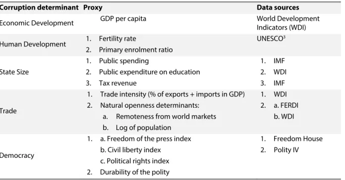
Table 1. Corruption determinants and data sources
Corruption determinant Proxy Data sources
Economic Development GDP per capita World Development
Indicators (WDI) Human Development 1. Fertility rate
2. Primary enrolment ratio
UNESCO3
State Size
1. Public spending
2. Public expenditure on education 3. Tax revenue
1. IMF 2. WDI 3. IMF
Trade
1. Trade intensity (% of exports + imports in GDP) 2. Natural openness determinants:
a. Remoteness from world markets b. Log of population
1. WDI 2. a. FERDI
b. WDI
Democracy
1. a. Freedom of the press index b. Civil liberty index
c. Political rights index 2. Durability of the polity
1. Freedom House 2. Polity IV
2 Mechanisms underpinning the effect of these determinants are discussed in Section 4. 3 Drawn from Teorell et al.’s (2015) database, University of Gothenburg.
3.4. Empirical specification
Pooled three-level estimations of the following baseline econometric model are conducted:
, , . . , , , , (4)
Subscripts i j, k refer to countries, sector, and firms respectively. Bribei,j,k is the variable of bribe
prevalence, Xi the vector of country-level corruption determinants, Yi,j,k the vector of micro-level
controls, dj the sector dummies, and εi,j,k a zero-mean constant-variance error term.
Three-level country-sector-firm maximum-likelihood estimations of equation (4) are conducted. When the binary variable of corruption incidence is used as a dependent variable, I perform a probabilistic linear multi-level modelling of equation (2), in order to avoid convergence problems (Caudill, 1988).4 If the sign and significance of the resulting estimated coefficients is informative, I
do not dare interpret their strength.
4. Empirical analysis
This empirical analysis starts by questioning the negative contribution of the economic development process to corruption prevalence. While income per capita is usually found to explain a significant part of cross-country differences in corruption prevalence, this relationship is not clear-cut and hides complex and sometimes conflicting mechanisms. Then, four additional mechanisms that could underlie the development-corruption nexus are discussed and tested within a three-level empirical framework: human capital, state interventions, openness, and democracy.
4.1. Is economic development detrimental to corruption?
The development process is considered a major determinant of corruption prevalence in the empirical literature. It is commonly argued that wealthier countries undergo less corruption, because corruption decreases with improved life standards, on the one hand; and because of the many institutional, sociological, and demographic changes which usually accompany the development process, on the other hand (Treisman, 2000).
However, putting aside the endogenous nature of the relationship, the development-corruption nexus is a catch-all phenomenon reflecting various and sometimes antagonistic mechanisms. In fact, higher income leads to a range of improvements in human capital, public resources managements, the rule of law, and so on, which are expected to drag down corruption levels, but these socio-economic transformations may also create new grounds for corrupt transactions
4 Probably due to the presence of dummy variables in our model, a convergence problem arises when a nonlinear mixed
(Andvig, 2006). From these two competing arguments, it is possible to derive the following opposite hypotheses:
H1: Corruption will be lower in more economically developed countries, when populations are less needy, more educated, when the management of public resources is efficient, and when institutions are better.
H1’: Corruption will grow with economic development, when new opportunities to enrich are not framed within the rule of law, when public funds are allocated with discretion, and when citizens cannot properly monitor public decision-making.
In order to have a proper assessment of the effect of GDP per capita on corruption prevalence, three-level estimations using WBES data on firms’ bribe reports are run and compared to single-level estimations. Results of valid multi-single-level models5 are presented in Table 2. When the bribe
payment (BP) dependent variable (continuous) is used, three-level estimations are compared to OLS estimations. When the bribery incidence (BI) variable (binary) is used, three-level estimations (linear probability model) are compared to Logit estimations. In a first step, corruption dependent variables are regressed over firms’ characteristics; the GDP per capita variable being included in a second step.
First, random intercepts are all found to significantly vary across countries and sectors, even though intra-class correlation coefficients6 – which inform the proportion of variance explained at
the country and sector levels – indicate that most of the variance is explained at the firm-level. However, intra-class correlation is substantial when the bribery incidence variable is used, as around 15%-20% of the variance is explained by within-country variations. Second, estimations stress the negative contribution of firms’ total sales and the positive contribution of their indirect exports to bribery. Access to external finance and internal funding are both found to deter firms’ bribery, while the share of public ownership is found to reduce corruption incidence.7
Third, the last two sets of regressions highlight the significant negative effect of income per capita on bribery. Single and multi-level estimates show that increased GDP per capita reduces both the average amount and the incidence of bribery in a sample of 71 developing countries. According to the third set of estimations, a 10% increase in the average GDP per capita results in a 0.67 percentage point decrease in the size of informal payments (see Figure 1), which is substantial, as the country average informal payments lies around 1.3% of firms’ total sales (see Appendix A).
5 Models with significant random components.
6 The country-level and sector –level intra-class correlation coefficients are calculated as follow:
ρ , and ρ
With σ , σ and σ the variance estimates of the country-level random intercept, the sector-level random intercept, and the residual, respectively.
7 This latter finding is consistent with the findings of Hellman et al. (2003), who show that public firms resort to influence
To conclude this sub-section, economic development is negatively and strongly related to corruption prevalence, but this evidence does not tell much about its transmission channels. In what follows, I test whether the human capital is an important channel for the relationship between income and corruption, by emphasizing the role of fertility and education in curbing corruption.
Figure 1. GDP per capita and bribe payments
4.2. Human capital and corruption
The New Economic Growth Theory considers long-run growth as being endogenously determined by demographic factors (Brezis & Young, 2014). In parallel, it has been stressed that demographic change is closely related to human capital evolution (Li et al., 2013; Becker & Tomes, 1994), and that a healthy and educated population is necessary for the well-functioning of institutions (Acemoglu et al., 2001; Glaeser et al., 2004; Svensson, 2005). To check whether the wealth-corruption nexus previously evidenced relies on the human development process, I run a second series of regressions including demographic and education variables8 together with the GDP per capita.
In a first step, the total fertility rate is used as a general proxy for human development, as changes in fertility are narrowly associated with the development process, more specifically with socio-economic changes that accompany the demographic transition. High fertility is indeed correlated with low access to health services and infrastructures, low educational attainment, a large and
youthful population, low wages, low productivity, and low saving rates (Varvarigos & Arsenis, 2015; Kuznets, 1960; Becker, 1960). As a result, high fertility rates may be a key determinant of corruption prevalence, by i) reducing quantities of public goods and services per capita, which may tempt citizens to bribe public agents to “jump the queue” (Banerjee, 1997; Fisman & Gatti, 2002); and by ii) reducing the empowerment of citizens, and therefore their ability to monitor public decision-makers. Therefore, the following hypothesis can be derived from these arguments.
H2: Corruption will be higher in countries with a large and low-skilled population, and will therefore increase with fertility rates.
A fertility rate variable is therefore introduced in the corruption equation (3) together with the GDP per capita. Three-level estimations using the bribe payment (BP) and the bribe incidence (BI) variables are reported in the first two sets of regressions in Table 3. In each set, I estimate the model with i) country/sector-level random intercepts only (the random intercept model), and ii) with country/sector-level random intercepts and random slope(s) (the random slope model). Only models with significant random parameters are reported.
The first two sets of regressions evidence a strong and significant positive effect of fertility rates on bribe payments and bribery incidence. Estimates with the BP variable reported in the first set of regressions show that the GDP per capita no longer has a significant effect once the fertility variable is introduced; thereby suggesting that human capital is a structural determinant of corruption and a critical channel of the GDP per capita-corruption nexus. Moreover, adding a random slope to the fertility parameter makes sense at the country-level with the BP and BI dependent variables, and at the sector-level with the BP dependent variable.
In a second stage, to check whether the effect of fertility passes through citizens’ empowerment, the specification is refined by adding a variable of basic educational attainment: the gross enrolment rate in primary school. A more educated population should indeed allow for a better monitoring of policies and rulers, but this effect may be ambiguous as more educated people may be correlated with increased rents in an economy (Eicher et al., 2009). The hypothesis testing is detailed below.
Table 2. Per capita income and bribery, single and three-level estimations
Dep. Var.: Bribe payments (1) Bribe incidence (2) Bribe payments (3) Bribe incidence (4)
OLS Multilevel Logit Multilevel OLS Multilevel Logit Multilevel
GDP per capita -0.0002*** (0.00002) -0.0002*** (0.0000) -0.0002*** (0.0000) -0.00003*** (0.0000) Firm controls
Log total sales 0.031 (0.031) -0.083*** (0.012) 0.027 (0.005) -0.0015* (0.0009) 0.011 (0.036) -0.093*** (0.018) 0.003 (0.033) -0.0031*** (0.001) % firms public ownership -0.002 (0.003) -0.0001 (0.003) -0.005* 0.003 -0.0005** (0.0002) -0.0001 (0.004) 0.001 (0.005) -0.005** (0.002) 0.0005 (0.0003) % indirect exports 0.012 * (0.007) 0.011*** (0.001) 0.003 (0.002) 0.0003** (0.0001) 0.004 (0.004) 0.006*** (0.002) 0.001 (0.002) 0.0003 (0.0001) % of direct exports -0.001 (0.001) 0.0004 (0.001) 0.0003 (0.002) 0.000 (0.000) -0.002 (0.002) 0.0001 (0.001) 0.002 (0.002) 0.0001 (0.0001) Internal fundinga -0.008*** (0.002) -0.007*** (0.001) -0.005*** (0.002) -0.001*** (0.0001) -0.008*** (0.002) -0.006*** (0.001) -0.006*** (0.001) -0.0006*** (0.0001) Bank fundingb -0.010*** (0.002) -0.003*** (0.001) -0.008*** (0.002) -0.0003*** (0.0001) -0.007*** (0.002) -0.0025* (0.001) -0.005** (0.002) -0.0001 (0.0001) Constant 1.184*** (0.34) 2.512*** (0.955) -0.308 (0.401) 0.017 (0.078) 2.103*** (0.548) 4.176*** (0.433) -0.510 (0.644) 0.409*** (0.042)
Dummies Firm size & sectors
Country level random
Intercept 2.988*** 0.046*** 3.018*** 0.050***
Intra-class corr. 2.4% 18.5% 1.77% 15%
Sector-level random effects
Intercept 0.278*** 0.002*** 0.338*** 0.002***
Intra-class corr. 0.02% 0.03% 0.02% 0.03%
(Pseudo)R2 / Wald 0.01 262.2*** 0.02 306.38*** 0.02 164.9*** 0.07 182.4***
LR Chi2 na. 3354.7*** na. 12071*** 1598.2*** 6779.2***
#Countries(Firms) 71(34,358)
H3: Corruption will be lower in countries with higher educational attainment, because a more educated population allows for better monitoring of public decision-making.
H3’: Corruption will be higher in countries with higher educational attainment, because a more educated population leads to the creation of new rents in the economy.
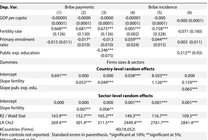
The last two regressions in Table 3 test the education channel alone. Fertility and education variables are then introduced together with the GDP per capita. Estimates are reported in Table 4 (columns (1), (2), (4), (5)). Once controlling for schooling and including a country-level random slope, a higher fertility rate is found to increase bribe payments but to reduce bribery incidence. Therefore, including a random component in the fertility coefficient slope reverses the sign of its estimated effect on BI, suggesting that the direct effect of fertility on BI is strongly affected by country-level unobserved heterogeneity. Moreover, estimates in column (5) of Table 4 support that the positive effect of fertility on BI evidenced in Table 3 (column (6)) is mainly channelled through educational attainment.
Regarding educational attainment, this primary enrolment rate is found to reduce bribe payments but to increase bribery incidence (Tables 3 and 4). Perhaps this variable provides a quantitative rather than qualitative assessment of educational attainment, and the positive effect of schooling on bribe incidence may result from the increase in rents induced by large pupil inflows in public schools. To examine this possibility, I introduce into the corruption equation a policy variable measuring the share of public expenditures on education in GDP.9 Estimates of valid models are
presented in columns (3) and (6) of Table 4. Once public expenditures on education are taken into account, the positive effect of primary enrolment and the negative effect of fertility on bribery incidence disappear (column (6)). An interesting fact is that the contrasting effect of primary enrolment on bribery evidenced in columns (2) and (5) is now reflected in the contrasting effect of public expenditures on education. This finding therefore highlights the ambiguous effect of schooling on corruption prevalence: while an educated population may improve the monitoring of public officials and thereby reduce the amounts of the latter may extract form their rents (H3), it may increase the number of corrupt transactions by increasing the size of public spending (H’3).
To sum up, the relationship between the development process and corruption is not as straightforward as surmised. Contrary to conventional wisdom, the growth process may create new opportunities for corrupt transactions at early stages of development, when citizens are not sufficiently empowered to scrutinize public actions, and when governments may be overwhelmed by an increasing demand for public goods and services. In this regard, previous results pointed out the role of increased public spending in channelling the positive effect of human development on corruption levels. The next section therefore further addresses the relationship between state interventions and corruption.
Table 3. Human Capital and bribery (1)
Dep. Var. Bribe payments (BP) Bribe incidence (BI) BP BI
(1) (2) (3) (4) (5) (6) (7) (8) GDP per capita -0.00003 (0.00007) -0.00001 (0.00004) -0.00003 (0.00006) 0.00001 (0.00004) -0.00002** (0.00001) -0.00001 (0.00001) -0.0003*** (0.0001) -0.00003*** (0.0000) Fertility rate 0.673*** (0.132) 0.697*** (0.137) 0.652*** (0.131) 0.681*** (0.138) 0.057*** (0.021) 0.067*** (0.028) Primary enrolment ratio -0.013 (0.012) 0.005*** (0.002)
Dummies Firms sizes & sectors
Country-level random effect parameters
Intercept 0.786*** 0.000 0.744*** 0.000 0.028*** 0.002*** 1.086*** 0.044***
Slope fertility 0.062*** 0.061*** 0.020**
Sector-level random effect parameters
Intercept 0.000 0.000 0.000 0.000 0.001*** 0.001*** 0.008*** 0.001***
Slope fertility 0.007*** 0.007*
R2 / Wald Stat 166.5*** 154.7*** 157.8*** 146.9*** 143.2*** 130.6*** 137.4*** 143.7*** LR Chi2 342.4*** 354.9*** 348.8*** 360.7*** 2935.8*** 2946.2*** 434.0*** 2601.9***
#Countries (#obs) 40(18.052)
Firm controls not reported. Standard errors in parenthesis. *significant at 10%; **significant at 5%; ***significant at 1%.
Table 4. Human Capital and bribery (2)
Dep. Var. Bribe payments Bribe incidence
(1) (2) (3) (4) (5) (6) GDP per capita -0.00005 (0.0001) -0.0000 (0.0001) -0.0000 (0.0001) -0.00001 (0.0001) -0.000 (0.0001) -0.000 (0.0001) Fertility rate 0.668*** (0.126) 0.681*** (0.130) 0.675*** (0.126) 0.005*** (0.002) -0.758*** (0.328) -0.071 (0.160) Primary enrolment ratio -0.015 (0.011) -0.017* (0.010) -0.013 (0.010) 0.059*** (0.024) 0.044*** (0.015) 0.003 (0.011)
Public exp. education -0.246***
(0.075) 0.212** (0.93)
Dummies Firms sizes & sectors
Country-level random effects
Intercept 0.691*** 0.000 0.000 0.038*** 8.503*** 0.000
Slope fertility 0.053*** 0.049*** 1.126*** 0.159***
Slope pub. exp. edu. 0.065***
Sector-level random effects
Intercept 0.000 0.000 0.000 0.001*** 0.001*** 0.001***
Slope fertility 0.007** 0.006**
R2 / Wald Stat 163.9*** 152.7*** 165.2*** 149.3*** 116.7*** 109.5***
LR Chi2 269.4*** 301.4*** 311.5*** 2449.4*** 2761.7*** 2841.4***
#Countries (Firms) 40(18.052)
Firm controls not reported. Standard errors in parenthesis. *significant at 10%; **significant at 5%; ***significant at 1%.
4.3. Are larger states more corrupt?
Over the last decades, state interventions in the economy and the oversize of the public sector have been pinpointed as being a major source of corruption. In contrast, the expansion of market-based transactions through increased domestic and foreign competition – i.e. deregulation, the privatization of state-owned enterprises, and trade openness – have been viewed as a lever for dragging firms’ profits down and therefore discouraging bribe payments (Shleifer & Vishny, 1993; Lambsdorff, 2005; Sandholtz & Koetzle, 2000; Ades & Di Tella, 1999).
In fact, a large public sector size is often depicted as a burden that incites private and public agents to exploit it or to get rid of it through malpractices. Notably, red tape10 may foster bribery of
bureaucrats in order to “get things done” or “to make things go faster” (Guriev, 2004; Aidt, 2003; Lambsdorff, 2002; Tanzi, 1998). Moreover, increased public expenditure may enlarge the scope of public resources under the discretion of public agents charged with their allocation, while higher tax rates may raise the amount of bribes asked or offered for tax exemption and evasion (Gauthier & Goyette, 2014; Gauthier & Reinikka, 2006; La Porta et al., 1999; Tanzi, 1998). For all these reasons, an increased scope for state interventions may increase the size of the “corruption pie”.
However, several arguments in support of there being a deterrent effect of public action on corruption can be invoked. Indeed, it has been contended that increased state intervention often tracks the long-run growth process (Peacock & Scott, 2000), generally accompanies the openness of economies (Rodrik, 1998), and sometimes results from improved economic and democratic institutions (Rodrik, 2000). Moreover, red tape does not systematically create opportunities for corruption since it may also be associated with better screening and higher internal administrative controls (Wilson, 1989). The effect of taxation also has to be nuanced since higher tax revenue may result from higher tax rates, but also from a larger tax base or a better firm tax compliance (Hibbs & Piculesco, 2010). Last but not least, it is argued that the growth of the private sector, illustrated by the wave of privatizations in the 90’s has increased the supply of corrupt transactions (Transparency International, 2009; Rose-Ackerman, 2007). It is therefore possible to derive two competing hypotheses over the state size-corruption nexus.
H4: Corruption will be higher in countries with greater state interventions if these interventions result in stronger monopoly and discretionary powers over public rents.
H4’: Corruption will be lower in countries with greater state interventions, if these interventions result in efficient public goods and service delivery and effective regulation of market-based transactions.
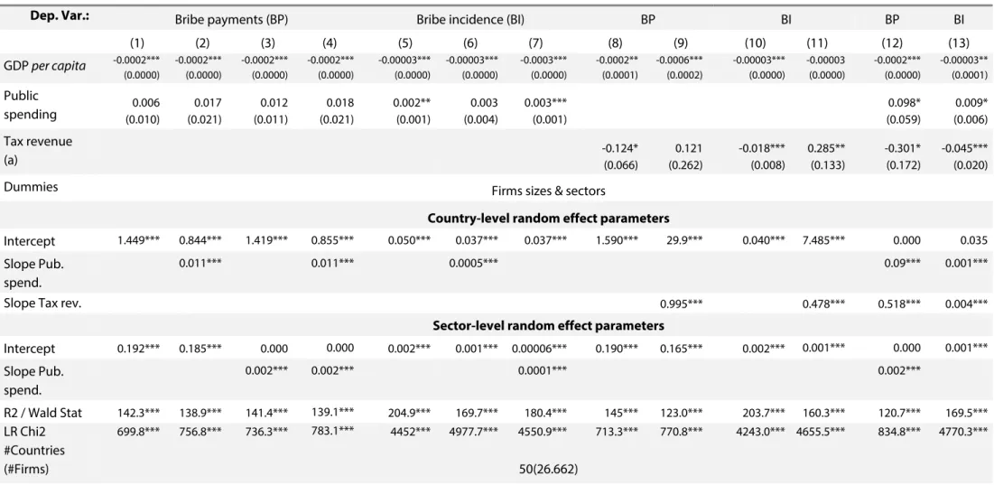
To test H4 against H4’, the share of public expenditure in GDP is used as a first proxy for public sector size, and is introduced alongside the GDP per capita in the corruption equation. Estimates of valid models are reported in the first two sets of estimates in Table 5 (columns (1) to (7)). Results show that there is no evidence of a significant effect of public expenditure on bribe payments. A
10 Red tape refers to excessive and/or poorly-designed bureaucratic rules that imply non-pecuniary costs for agents
positive significant effect of public spending on bribe incidence (second set of regressions) is found with the random intercept (column (5)) and the sector random-slope models (column (7)), but is no longer significant with the country random-slope model.
Moreover, because i) public spending may affect corruption through increased tax burden, and ii) public spending and taxation may have distinct effects on corruption prevalence, I use as a second proxy for public sector size: the share of revenue collected from goods and services (G&S) taxation in GDP.11 This variable is tested alone with GDP per capita (columns (8) to (11)), and then tested
jointly with the public expenditure variable (columns (12) and (13)). Random intercept models (columns (8) and (10)) support a negative effect of G&S taxation on corruption, suggesting that higher tax revenue results in lower bribe prevalence (Hibbs and Piculescu, 2010). However, including a country-level random slope component neutralizes this negative effect of tax on bribe payments (column (9)), and even reverses it into a significant and positive effect on bribery incidence variable (column (10)). This uncertainty over the coefficient sign is finally lifted up when public expenditure and tax revenue variables are introduced together in the random slope models (columns (12) and (13)). Each variable is found to have a separate effect on corruption outcomes: while a 10% increase in tax revenue results in a 3% decrease in the average bribe payment, a 10% increase in public expenditure is found to raise the average bribe payment by 1%.
In other words, the positive effect of increased tax revenue on bribe incidence evidenced in column (11) seems to be channelled through the effect of increased public spending on rent-seeking and corruption, highlighted in the literature. Once this latter effect is taken into account, the net effect of tax revenue on bribery is negative and may reflect the positive effect of the quality of tax policies and tax administrations on firm integrity or public spirit.
Despite this contrasting evidence on the effect of public sector “oversize” on corruption prevalence, the principles of competition that guided international institutions’ agenda towards a lower scope for public interventions were the same ones that motivated policies supporting increased openness of domestic markets. The effect of trade openness on bribery is therefore discussed and analysed in the next sub-section.
4.4. Are opened states less corrupt?
In the same way as excessive taxation has been depicted as a source of corruption by increasing the amount of bribes required for tax exemption (La Porta et al., 1999; Tanzi, 1998), higher trade barriers may create opportunities for politicians and customs officers to extort money or to sell favourable treatments to domestic and international private companies (Dutt & Traca, 2010; Gatti, 2004; Hellman, et al., 2003). Therefore, trade openness is expected to reduce the number and the size of corrupt transactions through lowered trade barriers and increased foreign competition. Moreover, Wei (2000) stressed that “natural openness”, i.e. trade openness determined by structural factors such as country size and geography, is associated with stronger institutional
safeguards against corruption. The author argues that countries’ natural inclination to trade incites governments to invest in institutions that protect foreign investors and traders from corrupt practices. Therefore both structural and policy-induced trade openness is likely to be detrimental to corruption.
However, Knack and Asfar (2003) have shown that the negative effect of trade on corruption is due to a selection bias in the country-coverage of corruption perception indices, which tend to under-represent poorly governed small nations. Moreover, over the last decades, the worldwide privatization of public services along with the removal of barriers to trade and financial flows has created a fertile ground for the internationalization of private corrupt practices, especially towards countries with weak and/or non-democratic institutions (Transparency International, 2009; Nellis, 2009; Hellman et al., 2003). Bribery is indeed a common and widespread means for international companies to win contracts abroad, to avoid regulations, or to unduly influence policy-making, especially in the developing and transition world (Hellman et al., 2003). Therefore, it is possible to derive from these arguments two competing hypotheses on the trade openness-corruption relationship.
H5: Corruption will be lower in opened economies, since lower trade barriers, foreign competition, and larger natural openness are detrimental to corruption.
H5’: Corruption will higher in opened economies, since trade openness exposes countries to imported foreign corrupt practices.
Table 6 reports three-level estimates of the effect of trade openness and bribe payments and incidence. First, a variable of trade intensity – the ratio of export plus imports on GDP – is included together with the GDP per capita in the corruption equation. A significant and positive effect on bribery incidence is evidenced, but no significant effect on the size of bribe payments. Second, public expenditures and tax revenue variables are included as a control to test whether the effect of trade openness on bribery depends on the size of a government. As pointed out by Rodrik (1992), the positive effect of trade openness on economic performance is uncertain, and its deterrent effects on corruption prevalence may depend on the extent of state interventions (Rodrik, 1998), so that previous estimations may suffer from omitted variable bias. Results in columns (3) and (6) put in evidence a direct positive effect of trade intensity the size of bribe payments and an indirect effect passing through the size of public interventions. Last, to check whether the effect of natural or structural openness (Wei, 2000) could interfere with the sign and significance of estimated relationships, an index of remoteness from world markets12 and a proxy
for country size (the logarithm of the population) are added into the corruption equation. Results are reported in columns (7) and (8). Including these variables in the regression highlights the positive and significant contribution of remoteness from world markets to bribe prevalence, and
12 Remoteness is an index between 0 and 100. It is the trade-weighted average distance from the nearest countries to
reach 50% of the world market, and adjusted for landlockness. This index is used by the UN-DESA for the calculation of the Economic Vulnerability Index and its methodology is presented here: http://byind.ferdi.fr/en/indicator/evi/build
makes the effect of the trade intensity on bribe payments insignificant. Therefore, these estimations suggest that i) trade openness has a direct effect on bribery relying on the country’s remoteness from world markets and independent from state interventions, and that ii) trade openness has an indirect effect on bribery, mediated by the size of state interventions.
These results are consistent with Rodrik’s (1998) findings that successful experiences of integration into international trade are often accompanied by larger state interventions. They also support the findings of Wei (2000), who stresses that remote countries face structural handicaps that preclude them from building good institutions. Interestingly, these authors also point out the importance of democratic institutions to make state interventions efficient and to cushion the economic turmoil resulting from international trading. The next section examines the link between democracy and corruption prevalence.
Table 5. State interventions and bribery
Dep. Var.: Bribe payments (BP) Bribe incidence (BI) BP BI BP BI
(1) (2) (3) (4) (5) (6) (7) (8) (9) (10) (11) (12) (13) GDP per capita -0.0002*** (0.0000) -0.0002*** (0.0000) -0.0002*** (0.0000) -0.0002*** (0.0000) -0.00003*** (0.0000) -0.00003*** (0.0000) -0.0003*** (0.0000) -0.0002** (0.0001) -0.0006*** (0.0002) -0.00003*** (0.0000) -0.00003 (0.0000) -0.0002*** (0.0000) -0.00003** (0.0001) Public spending 0.006 (0.010) 0.017 (0.021) 0.012 (0.011) 0.018 (0.021) 0.002** (0.001) 0.003 (0.004) 0.003*** (0.001) 0.098* (0.059) 0.009* (0.006) Tax revenue (a) -0.124* (0.066) (0.262) 0.121 -0.018*** (0.008) 0.285** (0.133) -0.301* (0.172) -0.045*** (0.020)
Dummies Firms sizes & sectors
Country-level random effect parameters
Intercept 1.449*** 0.844*** 1.419*** 0.855*** 0.050*** 0.037*** 0.037*** 1.590*** 29.9*** 0.040*** 7.485*** 0.000 0.035 Slope Pub.
spend.
0.011*** 0.011*** 0.0005*** 0.09*** 0.001***
Slope Tax rev. 0.995*** 0.478*** 0.518*** 0.004***
Sector-level random effect parameters
Intercept 0.192*** 0.185*** 0.000 0.000 0.002*** 0.001*** 0.00006*** 0.190*** 0.165*** 0.002*** 0.001*** 0.000 0.001*** Slope Pub. spend. 0.002*** 0.002*** 0.0001*** 0.002*** R2 / Wald Stat 142.3*** 138.9*** 141.4*** 139.1*** 204.9*** 169.7*** 180.4*** 145*** 123.0*** 203.7*** 160.3*** 120.7*** 169.5*** LR Chi2 699.8*** 756.8*** 736.3*** 783.1*** 4452*** 4977.7*** 4550.9*** 713.3*** 770.8*** 4243.0*** 4655.5*** 834.8*** 4770.3*** #Countries (#Firms) 50(26.662)
Table 6. Trade openness and bribery BP BI BP BI (1) (2) (3) (4) (5) (6) (7) (8) GDP per capita -0.0002*** (0.00004) -0.0002*** (0.00004) -0.0003*** (0.0001) -0.00003*** (0.000) 0.000 (0.0000) -0.0003*** (0.0001) -0.0003* (0.0001) -0.00003** (0.0001) Trade intensity (% of GDP) 0.0005 (0.006) 0.0009 (0.006) 0.033** (0.016) 0.002*** (0.0006) 0.024* (0.013) 0.002 (0.007) 0.027 (0.017) 0.002 (0.002) Pub. spend 0.095* (0.056) 0.009* (0.006) 0.096* (0.053) 0.009* (0.006) Tax rev.(a) -0.277* (0.167) -0.042** (0.020) -0.574*** (0.204) -0.055*** (0.022) Remoteness index 0.095*** (0.034) 0.007* (0.004) Log population 0.002 (0.163) 0.010 (0.019)
Dummies Firm size & sectors
Country-level random effect parameters
Intercept 1.831*** 1.426*** 0.000 0.053*** 20.837*** 0.029 0.000 0.029
Slope Trade 0.003***
Slope Pub spending 0.079*** 0.0007*** 0.062*** 0.0007***
Slope Tax revenue 0.486*** 0.004*** 0.518*** 0.004***
Sector-level random effect parameters
Intercept 0.345*** 0.000 0.000 0.002*** 0.001*** 0.001*** 0.000 0.001*** Slope Trade 0.0000*** Slope public spending 0.002*** 0.002*** R2 / Wald Stat 160.2*** 136.2*** 119.5*** 182.7*** 158.0*** 171.2*** 127.3*** 152.2*** LR Chi2 1108.2*** 750.0*** 838.0*** 6144.9 4833.0*** 4703.3*** 759.4*** 4264.1*** #Countries (#obs) 50(26,662) 47(23,116)
Controls not reported. Standard errors in parenthesis. *significant at 10%; **significant at 5%; ***significant at 1%. (a) General goods and services tax revenue.
4.5. Are democratic institutions detrimental to corruption?
The lack of accountability and transparency in public decision-making is a feature shared by corrupt and non-democratic countries. By supporting effective economic regulations and administrative rules, transparent procedures, law-enforcement institutions, and strong watchdog and oversight bodies, democracy represents a strong corruption deterrent. Democratic institutions indeed reduce opportunities for corrupt transactions, by allowing for improved scrutiny of voters upon political decisions, fostering political competition and supporting the freedom of media (Lambsdorff, 2002; Treisman, 2000, 2007; Sandholtz & Koetzle, 2000; Bhattacharyya and Hodler, 2015). According to Sandholtz and Koetzle (2000), this virtuous effect of democracy on governance depends on how well institutionally established norms of democracy are. This idea is also supported by Treisman (2000, 2007), who shows that only democracies older than 40 consecutive years are significantly associated with lower corruption levels.
The relationship between democracy and corruption may, however, be unstable at intermediary levels of democracy, as pointed out by Treisman (2007, p. 228): “Perceived corruption always decreases as democracy increases from 3 to 1 on the FH scale or as authoritarianism softens from 7
to 6, but the effects of movements between 6 and 3 are more erratic”. Therefore, based on this literature, the following conflicting hypotheses on the effect of democracy on corruption can therefore be made:
H6: Corruption will be lower in well-entrenched democratic countries.
H6’: Corruption will be higher in countries experiencing a transition towards democracy.
As a first evidence of the effect of democracy on corruption, I separate the sample between democratic and less democratic countries, and test H4 against H4’, and H5 against H5’ in each sub-sample. Democratic and less democratic countries are identified according to Freedom House (FH)’s democracy’s status,13 which is based on three indices that reflect three dimensions of
modern democracies: the extent of civil liberties (CL), of political rights (PR), and the freedom of the press (FotP). Using the combined CL and PR country status on the one hand, and the FotP status on the other hand, countries are split between free countries and less-free countries (i.e. countries with partly free and non-free status). The effects of openness and state interventions are then re-estimated using these separate sub-samples. Results are reported in Table 7.
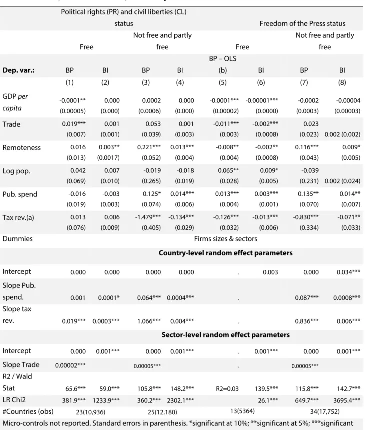
First, estimations show that, in PR-CL free countries (columns (1) and (2)), the effect of public spending and taxation is no longer significant, trade intensity significantly increases bribe payments, and remoteness fosters bribery incidence. In contrast, in PR-CL less-free countries (columns (3) and (4)), the effects of state interventions and remoteness are much stronger and more significant, while the effect of trade intensity is no longer significant. Therefore, the effects of natural openness and state interventions evidenced in Table 6 are found to mostly hold in less-free countries.
Second, when countries are split according to their FotP status (columns (5) to (8)), estimations highlight the virtuous effect of greater press freedom on trade-related variables. In fact, the effect of both trade intensity and remoteness on bribe payments and incidence turns negative and 1%-significant in countries with free press.14 In contrast, the effect of remoteness from world markets
on bribery is positive and significant in countries with a less-free press. Regarding domestic variables, the effects of state interventions on the economy are significant in both sub-samples, but stronger in the sample of FotP less-free countries than in the sample of FotP free countries.
In short, civil liberties and political rights on the one hand, and press freedom on the other hand appear as complementary corruption deterrent: while the former are found to neutralize the effect of internal determinants of corruption, i.e. related to state interventions, the latter is found to mitigate the effect of external trade-related causes of corruption. Moreover, estimations also show that the negative effect of GDP per capita holds in free countries, not in less-free countries.
13 Description of indices is given at https://freedomhouse.org/. The Press Freedom Index ranges from 0 (the most free) to
100 (the least free). The Civil Liberties and Political Rights Indices range from 1 (the most free) to 7 (the least free).
14 Since the LR test did not reject the superiority of the linear model over the multi-level model, I run instead OLS
To test the overall effect of democracy on bribe prevalence, CL, PR, and FotP indices are regressed together with the GDP per capita, within a random-slope three-level framework. Estimates15 are
reported in Table 8 (columns (1) to (8)) and are consistent across different valid calibrations of the random-slope model. They display contrasting evidence on the effect of these three dimensions of democracy on bribe prevalence. In fact, while increased political rights and media independence have, as expected, a significant deterrent effect on corrupt transactions, greater civil liberties are found to foster bribery. This last evidence suggests that the greater civil liberties may result in a larger scope for private initiatives, a larger private sector size, and hence an increased supply of bribes.
To explore this possibility, I enter into the corruption equation the four sub-indices from Freedom House, which are underlying the CL index: the rule of law index, the freedom of expression index, the associational rights index, and the personal autonomy index. If the positive effect of civil liberties on bribe prevalence passes through increased private initiatives, the latter index should be positively related to bribery. Estimates of the random slope model support a positive 5%-significant effect of personal autonomy on bribe payments (column (9)).
This contrasting evidence on the effect of democratic institutions on corruption questions the importance of the maturity of political systems for the study of the democracy-corruption nexus. In fact, this positive effect of personal autonomy on corruption prevalence may be explained by a larger scope for private corrupt transaction combined with the relative ineffectiveness of anti-corruption safeguards prevalent in young democracies (Treisman, 2000). To check whether the positive effect of personal autonomy holds when controlling for the longevity of political regimes, I add to the previous model a variable of polity durability drawn from the Polity IV database.16
Three-level estimates reported in columns (11) and (12) of Table 8 support a negative and significant effect of a political regime’s durability on bribe payments, but not on bribery incidence. More importantly, controlling for the durability of the polity neutralizes the positive effect of personal autonomy on bribe payments, as well as the negative effect of the rule of law on bribery incidence. This result therefore suggests that i) the stability of political institutions, whether democratic or not, is also a significant corruption deterrent and that ii) greater civil liberties in young democracies may lead to higher corruption levels because of an ineffective rule of law and larger scope for private transactions.
15 Their sign has been reversed so that their interpretation is not misleading, i.e. that a positive (negative) coefficient
reflects a positive (negative) effect on bribery.
16 The polity durability variable is the number of years since the most recent regime change or the end of transition
Table 7. Trade, state interventions, and bribery in free and less-free countries
Political rights (PR) and civil liberties (CL)
status Freedom of the Press status
Free
Not free and partly
free Free
Not free and partly free Dep. var.: BP BI BP BI BP – OLS (b) BI BP BI (1) (2) (3) (4) (5) (6) (7) (8) GDP per capita -0.0001** (0.00005) 0.000 (0.000) 0.0002 (0.0006) 0.000 (0.000) -0.0001*** (0.00002) -0.00001*** (0.0000) -0.0002 (0.0003) -0.00004 (0.00003) Trade 0.019*** (0.007) 0.001 (0.001) 0.053 (0.039) 0.001 (0.003) -0.011*** (0.003) -0.002*** (0.0008) 0.023 (0.023) 0.002 (0.002) Remoteness 0.016 (0.013) 0.003** (0.0017) 0.221*** (0.052) 0.013*** (0.004) -0.008** (0.004) -0.002** (0.0008) 0.116*** (0.043) 0.009* (0.005) Log pop. 0.042 (0.069) 0.007 (0.010) -0.019 (0.265) -0.018 (0.019) 0.065** (0.028) 0.009* (0.005) -0.039 (0.231) 0.002 (0.024) Pub. spend -0.016 (0.019) -0.003 (0.003) 0.125* (0.074) 0.014*** (0.006) 0.013*** (0.004) 0.003*** (0.001) 0.135** (0.070) 0.014** (0.007) Tax rev.(a) 0.013 (0.076) 0.006 (0.009) -1.479*** (0.405) -0.134*** (0.029) -0.126*** (0.032) -0.013*** (0.006) -0.830*** (0.334) -0.071** (0.033)
Dummies Firms sizes & sectors
Country-level random effect parameters
Intercept 0.000 0.000 0.000 0.000 . 0.003 0.000 0.034***
Slope Pub.
spend. 0.001 0.0001* 0.064*** 0.0004*** . 0.087*** 0.0008***
Slope tax
rev. 0.019*** 0.0003*** 1.066*** 0.004*** . 0.836*** 0.006***
Sector-level random effect parameters
Intercept 0.000 0.001*** 0.000 0.001*** . 0.001*** 0.000 0.001*** Slope Trade 0.00002*** 0.00005*** . 0.00005*** R2 / Wald Stat 65.6*** 59.0*** 105.8*** 148.2*** R2=0.03 139.5*** 115.8*** 142.7*** LR Chi2 381.9*** 1233.9*** 360.2*** 2302.1*** 26.1*** 649.7*** 3695.4*** #Countries (obs) 23(10,936) 25(12,180) 13(5364) 34(17,752)
Micro-controls not reported. Standard errors in parenthesis. *significant at 10%; **significant at 5%; ***significant at 1%. (a) General goods and services tax revenue. (b) OLS regression with standard errors robust to
Table 8. Democracy and bribery
Dependent variable: Bribe payments (BP) Bribe incidence (BI) BP BI BP BI
(1) (2) (3) (4) (5) (6) (7) (8) (9) (10) (11) (12) GDP per capita -0.0001*** (0.00004) -0.0001*** (0.00004) -0.0002*** (0.00004) -0.0001*** (0.00004) -0.00003*** (0.0000) -0.00002*** (0.0000) -0.00004*** (0.0000) -0.00003*** (0.0000) -0.00006 (0.00005) -0.00003*** (0.0000) 0.000 (0.000) -0.00006** (0.00003) PR scores -0.419** (0.186) -0.203 (0.182) -0.350*** (0.176) -0.427*** (0.188) -0.149*** (0.033) -0.069*** (0.017) 0.026 (0.022) -0.134*** (0.037) -0.564*** (0.222) -0.247*** (0.041) -0.680*** (0.239) -0.091** (0.046) CL scores 0.774*** (0.181) 0.588*** (0.201) 0.757*** (0.179) 0.789*** (0.181) 0.107*** (0.018) 0.146*** (0.022) 0.097*** (0.018) 0.184*** (0.018) FotP scores -0.047*** (0.015) -0.060*** (0.015) -0.051*** (0.016) -0.049*** (0.016) -0.004** (0.002) -0.008*** (0.001) -0.010*** (0.003) -0.004 (0.003) -0.077*** (0.018) -0.004* (0.002) -0.079*** (0.021) -0.011*** (0.004) CL – associational rights -0.009 (0.085) 0.010 (0.008) 0.090 (0.095) 0.016 (0.020) CL – Freedom of express. -0.669*** (0.118) -0.121*** (0.015) -0.798*** (0.131) -0.100*** (0.029) CL – Rule of Law -0.110 (0.082) -0.046*** (0.011) -0.065 (0.095) -0.014 (0.021) CL – Personal autonomy 0.246** (0.104) 0.001 (0.014) 0.195 (0.126) 0.018 (0.025)
Durability of the polity -0.055***
(0.021)
-0.003 (0.007) Country-level random effect parameters
Intercept 0.586** 0.267 0.314 0.393 0.078*** 0.025*** 0.201*** 0.014 0.747 0.112*** 1.652*** 0.137*** Slope PR 0.163*** 0.138*** 0.015*** 0.014*** 0.169*** 0.018*** 0.168*** 0.005 Slope CL 0.189*** 0.000 0.002*** 0.008 Slope FotP 0.001*** 0.0002 0.0001*** 0.00002 0.000 0.000 0.000 0.000 Slope Durability 0.001***
Sector-level random effect parameters
Intercept 0.086*** 0.000 0.000 0.000 0.002*** 0.000 0.000 0.000 0.000 0.000 0.000 0.0002
Slope PR 0.019*** 0.000 0.0001*** 0.000 0.000 0.000 0.000 0.000
Slope CL 0.025*** 0.001 0.0001** 0.000
Slope FotP 0.0001*** 0.0001*** 7.1e-07*** 0.000 0.0001*** 6.5e-07** 0.0001*** 0.000
Wald Stat 201.5*** 202.3*** 199.6*** 197.7*** 218.4*** 279.9*** 208.7*** 185.5*** 223.7*** 296.2*** 219.4*** 313.9***
LR Chi2 1605.5*** 1592.9*** 1609.3*** 1620.7*** 6836.4*** 6524.1*** 6818.3*** 6841.1*** 1456.6*** 6116.0*** 1352.9*** 5542.6***
#Countries (#obs) 71(34,358) 63 (33,337)
Micro-controls and dummies for firm size and sector of activity are included but not reported. Standard errors in parenthesis. *significant at 10%; **significant at 5%; ***significant at 1%.
5. Conclusion
Corruption results from individual choices, but these choices are also influenced by norms of ethics, trust, and coordination that prevail in a given society or a social group. Corrupt micro-level decisions may therefore be related to each other. In a micro empirical analysis, this interdependence of corruption decisions can be addressed through the multi-level modelling of corruption data. In a first step, a literature review sheds light the contextual nature of corrupt transactions and motivates the multi-level analysis of corruption prevalence. In a second step, an empirical study of the contribution of key corruption determinants emphasized by the economic literature is conducted within a three-level empirical framework.
In line with previous empirical research, multi-level estimates support that economic development, measured by income per capita, significantly and negatively contributes to bribery prevalence. However, this straightforward relationship hides complex and sometimes conflicting mechanisms. First, estimations highlight that this negative effect of income appears to be mostly driven by change in human capital-related factors, which in turn have a contrasting effect on corruption, partly mediated by the size of public spending (Eicher et al., 2009). Second, estimations show that state interventions have strong, but again contrasting, effects on corruption: while larger public expenditures increase corruption prevalence, higher tax revenues are negatively associated with corruption. This evidence suggests that an increased scope for state intervention may stimulate rent-seeking behaviours by inducing redistribution (Tanzi, 1998; Tornell & Lane, 1999), but on the other hand, increased state interventions often track the institutional development process (Peacock & Scott, 2000; Rodrik, 2000). Third, results stress that trade openness is partly mediated by state interventions but also by structural factors, such as countries’ geographical distance from world markets. These results therefore find an echo in the conclusions of Rodrik (1992, 1998), who stresses the role of government size for trade policy performances, and those of Wei (2000), who highlights the contribution of natural openness to the quality of institutions. Last, estimations emphasize the direct and indirect effects of democratic institutions on bribe prevalence, and also stress contrasting evidence: while increased political rights and media independence have, as expected, a significant deterrent effect on corrupt transactions, greater civil liberties are found to foster bribery. This result corroborates the findings of Treisman (2007) and stresses the importance of the maturity of political systems for the study of the democracy-corruption nexus, suggesting that the transition towards democracy may temporarily widen a scope for private corrupt transactions.