Chasing zero variability in software performance

(1)

Chasing Zero Variability in Software Performance

by

Severyn Kozak

Submitted to the Department of Electrical Engineering and Computer

Science

in partial fulfillment of the requirements for the degree of

Master of Engineering in Electrical Engineering and Computer Science

at the

MASSACHUSETTS INSTITUTE OF TECHNOLOGY

May 2020

c

○ Massachusetts Institute of Technology 2020. All rights reserved.

Author . . . .

Department of Electrical Engineering and Computer Science

May 1, 2020

Certified by . . . .

Charles E. Leiserson

Professor

Thesis Supervisor

Certified by . . . .

Tao B. Schardl

Research Scientist

Thesis Supervisor

Accepted by . . . .

Katrina LaCurts

Chair, Master of Engineering Thesis Committee

(2)

(3)

Chasing Zero Variability in Software Performance

by

Severyn Kozak

Submitted to the Department of Electrical Engineering and Computer Science on May 1, 2020, in partial fulfillment of the

requirements for the degree of

Master of Engineering in Electrical Engineering and Computer Science

Abstract

The ability to understand and control software performance variability is important for writing programs that reliably meet performance requirements. It is also crucial for effective performance engineering because it allows the programmer to collect fewer datapoints and still draw statistically significant conclusions. This wastes less developer time and fewer resources, and additionally makes processes like autotuning significantly more practical. Unfortunately, performance variability is often seen as unavoidable fact of commodity computing systems. This thesis challenges that notion, and shows that we can obtain 0-cycle variability for CPU-bound workloads, and <0.3% variability for workloads that touch memory. It shows how a programmer might take an arbitrary system and tease out and address sources of variability, and also provides a comprehensive glossary of common causes, making it a useful guide for the practical performance engineer.

Thesis Supervisor: Charles E. Leiserson Title: Professor

Thesis Supervisor: Tao B. Schardl Title: Research Scientist

(4)

(5)

Acknowledgments

Thank you Professor Charles E. Leiserson, Dr. Tao B. Schardl, and Tim Kaler for their supervision.

Thanks to mom, dad, Tysia, and the rest of family for all the love and support.

Thanks to Tom, Jorge, Anton, Gannon, Pau, Collin, Elley, and all the rest for making the year memorable.

(6)

(7)

List of Figures

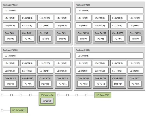
2-1 lstopovisualization of the hardware on an a1.metal instance. . . . 23

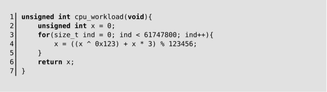
3-1 Simple CPU benchmark. . . 26

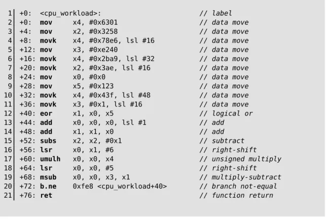
3-2 The assembly corresponding to Figure 3-1. . . 27

3-3 Runtimes on a quiet system. . . 29

3-4 Contents of /proc/interrupts(some text omitted). . . 30

3-5 Kernel module wrapper for our benchmark code. . . 31

3-6 Runtimes from the kernel module. . . 32

3-7 Contents of /proc/sched_debug for core #15. . . 34

3-8 kworkers in ps -efoutput. . . 35

3-9 Kernel command line that isolates CPUs and engages dynamic ticks. 38 3-10 Userspace runtimes on an isolated core demonstrating zero-cycle vari-ability. . . 39

3-11 Implementation of a prime number sieve, an example of CPU-bound code with heavy branching. . . 41

3-12 The assembly corresponding to Figure 3-11. . . 42

3-13 Branch-heavy code demonstrating eventual zero-cycle variability. . . . 43

4-1 A simple workload for assessing memory variability. . . 49

4-2 The assembly corresponding to the memory workload in Figure 4-1. . 50

4-3 Runtimes (with very tight error bars) for 300 trials of each of many combinations of number of memory accesses and working-set size. Note: logarithmic scale. . . 51

(12)

4-4 Running times of L1 Cache benchmark demonstrating intermittent in-terference due to user script running on unrelated core. . . 54 4-5 Performance variability with and without intermittent interference. . 55

5-1 Running times of the same workload run for consecutive trials, with and without clock-frequency scaling. . . 59 5-2 Running times of the same workload, with a twin hyperthreaded core

that is first busy and then idle. . . 60

(13)

List of Tables

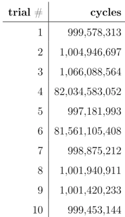
3.1 Variability obtained by each refinement of our testing environment. . 26 3.2 Runtimes on a busy system running make -j. . . 28

(14)

(15)

Chapter 1 Introduction

Software performance variability is often seen as an unavoidable fact of commodity computing environments. Run the same program ten times and you will likely see ten (very) different running times. Researchers attribute this to the fact that modern computing systems are full of complex features [1] designed to maximize the aver-age throughput of dozens, if not hundreds, of programs running concurrently. While these features improve overall system performance, they make it extremely difficult to obtain consistent performance for a single program. Even the simplest computa-tional workload faces interference from operating system preemption [2], interrupts [3], memory bandwidth congestion, address space layout [4], clock frequency throttling, and much more. More complicated programs have even more layers of variability, including (but certainly not limited to) unpredictable disk-access latencies, filesystem caches, and non-uniform memory access (NUMA).

The ability to understand and address sources of variability is important for sev-eral reasons: obtaining performance guarantees, simplifying performance engineer-ing, and knowing how to make our systems generally more performant. This thesis demonstrates how we can obtain zero-cycle variability for CPU-bound workloads and minimize variability for memory-bound workloads, and provides a glossary of different sources of variability and how they can be addressed.

Understanding variability lets us write software that consistently meets perfor-mance requirements. In the context of high-perforperfor-mance software, programmers

(16)

gen-erally care about a mixture of latency and throughput. For example, if a video game plays at a rate of 60 frames per second, then each physics update step must more-or-less reliably complete within ₆₀1th of a second, and consequently minimizes latency. Similarly, a middle-layer HTTP API within a large piece of web infrastructure might have a Service Level Agreement that demands certain latency and jitter guarantees. A database update running in the background might optimize more heavily for over-all throughput if its result is not immediately required. Other code must equover-ally prioritize both latency and throughput. Understanding and controlling variability is critical for ensuring these kinds of performance goals are met.

Obtaining consistent performance measurements means less noisy data, which makes performance engineering tremendously easier. In a noisy environment, a pro-grammer must collect many datapoints to have confidence that their code is indeed getting faster. This wastes both computing resources and programmer time, and also occasionally makes things like autotuning simply intractable because of the blowup that occurs from combining high dimensionality with the large number of necessary datapoints [5]. Reducing variability addresses all of these problems.

Controlling variability allows the programmer to improve the overall performance of their system. Any kind of variability experienced by a program is often due to avoidable noise. If we understand how to identify and mitigate this noise, we can shield our programs from interference and secure a performance improvement across the board.

Variability has been studied extensively, but existing research does not provide a coherent guide for taking a commodity system and using it to obtain hyper-consistent performance for deterministic workloads. Prior work has produced everything from software suites for reproducing performance variations [6], to machine learning tech-niques for diagnosing performance issues [7], to studies of how memory layouts impact performance [4, 8]. Becker and Chakraborty [1] provide an excellent glossary of the hardware and software features in an average computer that might cause variability. Oliveira, Petkovich, and Fischmeister [8] investigate a specific source of variability, memory layout. My research builds on existing work by providing a unified analysis

(17)

of many discrete sources of variability, the baseline amount of variability that we can expect from each one, and how we address them individually, with the aim of demonstrating an exploratory process of taking an arbitrary commodity system and identifying its sources of variability one-by-one.

My thesis research provides a comprehensive glossary of sources of variability, and demonstrates how one might go about mitigating variability for increasingly complex workloads. Importantly, the target environment is a “commodity computing system” – that is, general-purpose hardware paired with a general-use operating system, like a desktop or cloud machine, rather than a niche setup like a supercomputing cluster or a realtime operating system. In particular, I target bare-metal Amazon Web Services (AWS) servers with ARM processors running the Linux operating system. In this environment, I start off with a very simple CPU-bound workload, slowly scale it up by adding features that use additional parts of the hardware and operating system – branch prediction, memory accesses, etc. – and at each level see how well I can cope with the new variables. I find that I can obtain zero-cycle variability for CPU-bound workloads, and as low as 0.3% variability for workloads that touch memory. I believe this approach is useful both because it shows how a programmer might take an arbitrary new system and start teasing out the causes of noise, which otherwise may feel like a daunting problem with no clear starting point, and because it provides an extensive reference for sources of variability in general. This experimentation involves the interrupt subsystem, branch predictor implementations, tickless kernels, cross-machine memory interference, and more.

The structure of this thesis is as follows. Chapter 2 more thoroughly frames the problem, enumerating a sample list of sources of variability, describing the hardware and software used in my testing, and justifying my approach and testing methodology. Chapter 3 describes how I obtain consistent performance for a workload that runs en-tirely on the CPU without performing any data memory accesses. Chapter 4 describes how I minimize variability for workloads that make extensive data memory accesses. This concludes the hands-on story of how I reduced variability for increasingly com-plicated workloads. Chapter 5 provides a thorough glossary of different sources of

(18)

variability, and takes a closer look at each individual one (interrupts, hyperthreading, etc.). Chapter 6 concludes by summarizing my work.

(19)

Chapter 2 Background and Approach

The problem of variability is a daunting one, due to a large number of interleaved sources of variability that may be difficult to identify and separate out. We present examples of the kinds of variability we may see (Section 2.1), justify our experimental approach (Section 2.2), describe our testing environment (Section 2.3), and discuss our code and timing methods (Section 2.4).

2.1 A Sampler of Variability Sources

There are many orthogonal sources of variability in a typical computing environ-ment. The following list enumerates some important ones, and gives a sense of the complexity of the problem.

∙ CPU clock frequency scaling (e.g. Intel Turbo Boost): modern machines support clock frequency scaling (i.e. lowering and raising the frequency of the CPU clock), both to reduce power usage and to avoid overheating.

∙ Simultaneous multithreading (abbreviated as SMT; e.g. Intel Hyper-Threading): many modern CPUs have cores that support simultaneous multi-threading, or the semi-concurrent execution of two different instruction streams. This offers a speedup that varies between that of having one and two separate

(20)

cores, but also introduces room for processes running on mutually multithreaded cores to interfere with one another.

∙ Scheduler preemption: general-purpose operating systems are designed to concurrently execute dozens of user processes. Without special care, a user process will be frequently preempted by the operating system scheduler to allow other processes to run.

∙ Interrupts: a program can be preempted by more than just competing pro-cesses. At a lower level, interrupts are constantly getting delivered to each CPU, preempting the running process regardless of whether it has been isolated from preemption by other processes or not.

∙ Branch prediction: branch prediction revolves around maintaining a cache of branch instructions and their histories (“taken”/“not taken”). This can lead to variability depending on the initial state of the branch predictor cache when the user program starts execution.

∙ Memory cache contention: on multi-core CPUs, higher levels of cache (L2, L3) are generally shared between cores, which opens up the possibility of cache contention from processes running on other cores.

∙ Memory bandwidth contention: similarly, memory bandwidth is limited, and thus a memory-intensive process running on one core might be artificially throttled by memory-intensive processes running on nearby cores.

∙ Address Space Layout Randomization (ASLR): ASLR is a security mech-anism that randomizes the location of different segments of memory, making attacks like buffer overflow exploits more difficult. Unfortunately, it also results in potentially variable performance, in particular if it changes the way certain memory addresses map into cache.

∙ Non-Uniform Memory Access (NUMA) effects: in NUMA architectures, each core generally has its own physically proximal block of main memory,

(21)

and together these constitute a global view of main memory. The downside is that any one core has varying access latencies to different chunks of memory, depending on how far away they are, which introduces a source variability that is difficult to control for.

∙ Unpredictable disk latencies and filesystem cache: reading/writing the disk introduces a slew of additional problems. Disk latencies are relatively large and unpredictable, and the operating system will often cache the contents in memory to accelerate subsequent lookups.

∙ Memory refresh: DRAM constantly leaks charge and thus needs to period-ically refresh itself by reading values from cells and writing them back. This leaves it periodically unable to service requests and stalls the CPU, which can potentially lead to large variability in micro-benchmarks.

This list conveys the sheer challenge of tackling performance variability. Where do you begin? With so many interleaved sources, all of different magnitudes, how do you know if you are progressing in the right direction when tweaking your system? This thesis demonstrates that, while sources like clock frequency scaling or SMT are trivial to disable or prevent, others, like memory cache/bandwidth contention or branch prediction variability, are essentially unavoidable.

2.2 Tackling Variability Step-by-Step

Section 2.1 suggests that approaching the general problem of variability in our soft-ware requires the ability to isolate individual variables (like hyperthreading, or system calls, or network interrupts) so that we can investigate them independently. For that reason, my thesis adopts the following methodology:

∙ I start off with a very simple CPU-bound workload that performs simple math and logic operations on register values.

(22)

∙ I see how much I can reduce the variability of that workload. Any remaining variability is a sort of “baseline variability” that will manifest in any workload whatsoever on our system, because the workloads will only increase in complex-ity and pull in more potential sources of variabilcomplex-ity.

∙ One by one, I make the workload “more variable” by adding in what I suspect is a single additional source of variability. For example, first I add heavy use of the branch predictor. Then, I add substantial use of memory (which unfortunately pulls in several sources of variability that are hard to disentangle).

∙ At each step, I repeat the process of seeing how low I can get the variability. This reveals the baseline variability of each source.

2.3 The Environment

The computing environment consists of a commodity server running Ubuntu, a Linux-based operating system. I use the a1.metal instance type provided by Amazon Web Services (AWS), a large cloud provider. Importantly, a1.metal instances are “bare-metal” in that they provide complete, direct access to the hardware and memory of the system – the machines are single-tenant and do not have a hypervisor. This is important because we have no control over other users in multi-tenant setups and the interference they can cause by utilizing the same underlying hardware.

Figure 2-1 shows the layout of an a1.metal instance. Each instance has 16 ARM○c Cortex-A72 processors organized into 4 clusters of 4 cores each. Each core has a private L1 instruction cache (48KB) and L1 data cache (32KB). Each cluster of 4 cores has a shared L2 cache (2048KB), and the machine as a whole has 31GB of main memory. Note that the system does not have NUMA, i.e. all memory accesses go to a single, monolithic block of main memory. Moreover, cores do not have simultaneous multithreading (known as Hyper-Threading on Intel processors), nor does the system have DVFS enabled. Thus, two potential sources of variability are already dealt with.

(23)

Figure 2-1: lstopo visualization of the hardware on an a1.metal instance.

The instance runs Ubuntu 18.04.3 LTS, with Linux kernel version 4.15.0-1056-aws (an AWS patch of Linux 4.15.0).

2.4 Code and Time Measurement

All benchmark code is written in C, which allows us to easily cross-reference the code we write with the assembly it generates. When we “benchmark” a piece of code, we write that code into a function and run it some number of times (as few as ten and as many as a few thousand) within the same process. The running time of each execution is measured in CPU cycles, recorded by reading the CPU Cycles performance counter. Timing code this way is extremely fast and unintrusive. Unless otherwise stated, code samples are compiled with GCC version 7.5.0 and -O3 (maximal optimizations enabled).

(24)

(25)

Chapter 3 Zero Variability in CPU Workloads

This chapter demonstrates how the variability of a CPU-bound workload can be reduced from an almost unbounded worst-case value to exactly zero. The first step is to devise a workload (Section 3.1) and establish both a worst-case variability by running it on a busy system (Section 3.2), and a best-case variability by running it on a quiet system (Section 3.3). We then hypothesize that interrupts are causing our variability in both cases (Section 3.4), and test this by writing our benchmark into a kernel module that disables interrupts and find that we obtain zero-cycle variability (Section 3.5). Unfortunately, rewriting an arbitrary benchmark as a kernel module is impractical, so we investigate whether we can translate our results to user space. We find that by configuring the kernel via isolcpus, workqueue affinities, and IRQ affinities, we can obtain an almost identical setup (Section 3.6). The last step is to remove the timer tick, accomplished by building a Linux kernel with full “dynamic ticks,” or support for tickless cores (Sections 3.7 and 3.8). With this configuration we obtain zero-cycle variability for our CPU workload in user space. Finally, we explore variability in a branch-heavy CPU-bound workload, and find that we can obtain zero-cycle variability by warming up the branch predictor with trial runs (Section 3.10).

(26)

Table 3.1 shows the variability obtained by each refinement of our testing envi-ronment. version # variability busy system 10,000% quiet system 0.00001% kernel module 0% user space w/o dyn. ticks 0.001% user space w/ dyn. ticks 0%

Table 3.1: Variability obtained by each refinement of our testing environment.

3.1 CPU Workload

We devise a workload that resides entirely on the CPU. That is, outside of pulling instructions from memory, it performs no memory accesses and performs simple math-ematical and logic operations on values residing in registers. Figure 3-1 shows the C code. The “magic constants” are arbitrary and the whole function computes some sort of hash value.

1 unsigned int cpu_workload(void){

2 unsigned int x = 0;

3 for(size_t ind = 0; ind < 61747800; ind++){

4 x = ((x ^ 0x123) + x * 3) % 123456; 5 }

6 return x;

7 }

(27)

1 +0: <cpu_workload>: // label

2 +0: mov x4, #0x6301 // data move

3 +4: mov x2, #0x3258 // data move

4 +8: movk x4, #0x78e6, lsl #16 // data move

5 +12: mov x3, #0xe240 // data move

6 +16: movk x4, #0x2ba9, lsl #32 // data move

7 +20: movk x2, #0x3ae, lsl #16 // data move

8 +24: mov x0, #0x0 // data move

9 +28: mov x5, #0x123 // data move

10 +32: movk x4, #0x43f, lsl #48 // data move

11 +36: movk x3, #0x1, lsl #16 // data move

12 +40: eor x1, x0, x5 // logical or

13 +44: add x0, x0, x0, lsl #1 // add

14 +48: add x1, x1, x0 // add

15 +52: subs x2, x2, #0x1 // subtract

16 +56: lsr x0, x1, #6 // right-shift

17 +60: umulh x0, x0, x4 // unsigned multiply

18 +64: lsr x0, x0, #5 // right-shift

19 +68: msub x0, x0, x3, x1 // multiply-subtract

20 +72: b.ne 0xfe8 <cpu_workload+40> // branch not-equal

21 +76: ret // function return

Figure 3-2: The assembly corresponding to Figure 3-1.

Annotated assembly code corresponding to Figure 3-1 is shown in Figure 3-2. Note the singular branch instruction on line 20, and the otherwise simple data move/com-putation instructions.

3.2 Variability on a Busy System (Worst-Case)

We first want to establish a sense of the magnitude of variability we can see on a loaded system – after all, the average machine is often busy running background processes, handling network requests, writing the disk, and more. We simulate heavy load by building the Linux kernel from source [9] in the background with make -j [10], which parallelizes the build across all available cores.

(28)

and demonstrate tremendous variability. There is almost a 100x difference between some of the runtimes.

Although our method of simulating “system load” is extreme in that few systems are ever so busy on all cores for an extended period of time, it gives us a sense of what can happen to individual trials of a benchmark in the face of even a momentary spike in system activity. Without guarantees on how other work on the system interferes with our benchmark, we almost have no upper bound on how much variability we can exhibit. trial # cycles 1 999,578,313 2 1,004,946,697 3 1,066,088,564 4 82,034,583,052 5 997,181,993 6 81,561,105,408 7 998,875,212 8 1,001,940,911 9 1,001,420,233 10 999,453,144

Table 3.2: Runtimes on a busy system running make -j.

3.3 Variability on a Quiet System (Average-Case)

Next, we aim to understand our best case variability, i.e. the variability observed on a quiet system with minimal activity. Without the artifical make -j workload, our system is not doing much at all besides running some low resource background processes, many of which we can disable.

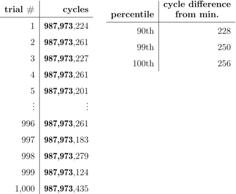
Running our benchmark on this relatively quiet system gives the extremely low variability times in Figure 3-3. The range is only 256 cycles (between trials #9 and

(29)

#10), which corresponds to an approximately 2.6 · 10−5% difference. From the stand-point of practical engineering, this is already very low, but it poses the question of whether we can achieve exactly zero-cycle variability. Moreover, while this particu-lar execution exhibited low variability, Section 3.2 demonstrates that an unexpected spike in system load could dramatically increase it. In other words, without hard guarantees of isolation, we cannot reliably expect low variability.

trial # cycles 1 987,973,224 2 987,973,261 3 987,973,227 4 987,973,261 5 987,973,201 .. . ... 996 987,973,261 997 987,973,183 998 987,973,279 999 987,973,124 1,000 987,973,435 percentile cycle difference from min. 90th 228 99th 250 100th 256

Figure 3-3: Runtimes on a quiet system.

3.4 What Causes Our Variability?

In the absence of simultaneous multithreading and clock frequency scaling, which are the main culprits in CPU-bound variability, we turn to interrupts as the most likely explanation of any variability we see. Processor interrupts by definition interrupt our workload to allow other things to run [11, ch. 7].

We can roughly split interrupts into two categories: non-timer interrupts, which are easy to get rid of, and timer interrupts, which are hard to get rid of. Timer interrupts run at a regular frequency and kick the scheduler into action, which checks,

(30)

for example, whether the current process has exhausted its time slice or whether a higher priority process is waiting to run. Timer interrupts also allow the system to collect CPU utilization statistics and more. Thus, the way Linux works out-of-the-box, per-core timer interrupts are unavoidable. All other frequent interrupts on our system, however, can be conceivably moved to a small subset of “housekeeping” cores [12], so that the cores running our benchmark code do not have to sporadically process interrupts from the network card or disk controller.

We can get a sense of the interrupts occurring on our system by reading the

/proc/interrupts file, which tells us the number of each type of interrupt delivered to each core in our system since boot [11, ch. 7]. For example, Figure 3-4 tells us that core 15 has processed 4,434 arch_timer (the name of the timer interrupt) interrupts since boot. We can also record the precise number of interrupts that arrive between two points in our code by reading the relevant CPU performance counters [13].

1 $ cat /proc/interrupts 2 CPU0 ... CPU15

3 1: 0 ... 0 GICv3 25 Level vgic 4 2: 6455 ... 4434 GICv3 30 Level arch_timer 5 3: 0 ... 0 GICv3 27 Level kvm guest vtimer 6 5: 0 ... 0 GICv3 147 Level arm-smmu global

7 6: 0 ... 0 GICv3 149 Level arm-smmu-context-fault, ... 8 8: 0 ... 0 GICv3 23 Level arm-pmu

9 ...

Figure 3-4: Contents of /proc/interrupts (some text omitted).

3.5 Disabling Interrupts with a Kernel Module

We can test whether interrupts are the source of our variability by running our bench-mark with interrupts disabled. Unfortunately, this is easier said than done. Interrupts are a low-level feature of the computing stack and largely invisible to the user. Some,

(31)

like the timer interrupt, are hardwired into the kernel. Note that this is the case for the Linux kernel – if we were using an operating system purpose built for e.g. real-time software, this would likely not be the case, since that operating system would optimize for exactly this usecase. Linux, on the other hand, requires taking intrusive measures to obtain this level of isolation.

While disabling interrupts is not possible from user space, it is certainly possible from kernel space [11, ch. 7]. Drivers and other critical sections of kernel code that cannot stand interruption do it all the time. Thus, we can write our benchmark into a kernel module. A kernel module is a piece of kernel code that can be loaded on demand, meaning we can write kernel code without having to modify and recompile the kernel. 1 #include <linux/init.h> 2 #include <linux/module.h> 3 #include <linux/kernel.h> 4 #include <linux/sort.h> 5 #include <linux/smp.h> 6 #include <linux/delay.h> 7 8 #include "cpu.h" 9 10 static DEFINE_SPINLOCK(lock); 11

12 static int __init lkm_example_init(void) {

13 unsigned long flags;

14 spin_lock_irqsave(&lock, flags); 15 runBenchmark(); 16 spin_unlock_irqrestore(&lock, flags); 17 return 0; 18 } 19

20 static void __exit lkm_example_exit(void){}

21

22 module_init(lkm_example_init); 23 module_exit(lkm_example_exit);

(32)

Writing a kernel module requires a boilerplate Makefile taken from the ker-nel documentation and some template code, as shown in Figure 3-5. The call to

spin_lock_irqsave(&lock, flags) disables interrupts, runBenchmark() runs the benchmark code (exactly the same code that we run in user space), and

spin_unlock_irqrestore(&lock, flags) re-enables interrupts.

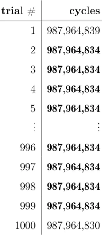
We find that the benchmark now exhibits zero-cycle variability. We compile and load this kernel module via insmod [14], and view its output in the kernel ring buffer via dmesg [15]. The runtimes are reported in Figure 3-6, and are essentially perfectly consistent. Ignoring the first and last trial, each one runs for exactly 987,964,834 cy-cles. The discrepancy in the first and last trial are likely due to a branch misprediction in the first and last iteration of the for-loop running the trials of the benchmark code – we can loosely verify this by increasing and decreasing the number of trials, and observing that it is always the first and last iteration that differ from the others, and also by looking at branch prediction performance counters.

trial # cycles 1 987,964,839 2 987,964,834 3 987,964,834 4 987,964,834 5 987,964,834 .. . ... 996 987,964,834 997 987,964,834 998 987,964,834 999 987,964,834 1000 987,964,830 percentile cycle difference from mode 90th 0 99th 0 100th 5

(33)

We can conclude that interrupts were causing our variability, and that disabling them lets us achieve zero-cycle variability in a CPU-bound workload.

3.6 Translating to Userspace

We investigate how to translate our results in Section 3.5 to user space, and find that a number of kernel configuration options bring us close. This is important because it is neither feasible nor recommended to convert every piece of benchmarkable code into a kernel module that disables interrupts. At the very least, it is an abuse of Linux and does not mirror the environment a user space application runs in. The options that prove useful to us are isolcpus, workqueue affinities, and IRQ affinities.

3.6.1 isolcpus

Our first tool is isolcpus [16], a kernel parameter that isolates certain cores from general scheduler activity. This allows us to prevent user processes from getting scheduled on a core, though it does nothing about kernel processes (like kworkers, for example, which perform work required by the kernel and are discussed in Sec-tion 3.6.2).

Adding isolcpus=8-15 to our kernel commandline via /etc/default/grub

isolates all cores in the range 8-15. If we run something like make -j again, we observe that that only cores 0-7 have make processes running on them.

We can consult /proc/sched_debug to see that the isolated cores only have kernel processes scheduled on them. /proc/sched_debug provides a wealth of per-core scheduling information, including a list of the processes scheduled on each per-core, as shown in Figure 3-4. In this case, we see that core 15 has only cpuhp, migration,

ksoftirqd, and kworker scheduled on it, all of which are instantiated by the kernel.

(34)

1 $ cat /proc/sched_debug 2 ... 3 cpu#15 4 .nr_running: 0 5 ... 6 runnable tasks: 7 S task PID ... 8 --- ... 9 S cpuhp/15 98 ... 10 S migration/15 99 ... 11 S ksoftirqd/15 100 ... 12 I kworker/15:0 101 ... 13 I kworker/15:0H 102 ... 14 I kworker/15:1 367 ... 15 I kworker/15:1H 1264 ...

(35)

3.6.2 Workqueue Affinity

We can partially isolate our cores from kernel threads by setting workqueue affinities. The kernel often creates work that has to be deferred, or needs to sleep(), or that simply needs to be fairly load balanced with all the other work that needs to be done. It places this work into “workqueues.” Kernel worker threads called kworkers retrieve the work placed in “workqueues” and perform it [11, ch. 8].

There are many kworkers on a given system. For example, ps -ef yields 67 different kworker threads, as shown in Figure 3-8. Threads are named in the format

kworker/cpu:idpriority; for instance, kworker/15:0H runs on core 15 with High priority.

1 $ ps -ef | grep -i kworker 2 ...

3 root 1757 2 0 Apr17 ? 00:00:00 [kworker/13:1H] 4 root 1758 2 0 Apr17 ? 00:00:00 [kworker/14:1H] 5 root 1759 2 0 Apr17 ? 00:00:00 [kworker/15:1H] 6 root 3670 2 0 03:34 ? 00:00:00 [kworker/u32:1-e] 7 root 4122 2 0 08:15 ? 00:00:00 [kworker/u32:0-e] 8 ...

Figure 3-8: kworkers in ps -ef output.

Some workqueues can be pinned to specific cores. In particular, workqueues cre-ated with the WQ_SYSFS parameter are exposed to the user via sysfs and accept a cpumask [17]. For example, the writeback workqueue can be pinned to cores 1 and 2 via echo 0003 > /sys/devices/virtual/workqueue/writeback/cpumask. Set-ting workqueue affinities like so prevents them from being processed on the cores that we want isolated.

However, not all workqueues are configurable by the user, and are an ple of an inherent kernel design choice that could lead to variability. For exam-ple, a simple grep of the Linux kernel source code turns up hundreds of calls to

(36)

alloc_workqueue(), only a few of which are created with WQ_SYSFS and thus exposed to the user. The rest could potentially be processed by kworkers on any core, meaning that our isolated cores might not be truly isolated. Since Linux is not specifically designed for our ultra low variability needs, it does not completely sup-port full core isolation, and short of modifying the kernel we cannot obtain a perfect guarantee of non-interference.

3.6.3 Disabling Unnecessary Services

Disabling unnecessary system services removes another potential source of variability. Even if a system service run as a user processes and thus can be isolated to a subset of cores via isolcpus (Section 3.6.1), it can trigger kernel work (like disk or network I/O) that is processed via workqueues. As mentioned in Section 3.6.2, it is not possible to isolate any core from all potential workqueue activity, and so it is important to minimize the likelihood of it occurring. Examples of system services that are likely superfluous for a benchmarking environment are update managers, package managers (e.g. snap), and job execution services (e.g. cron). Running processes can be easily viewed with tools like top or ps, and disabled via interfaces like service,

systemctl, a kernel parameter, or others (it depends on the particular service).

3.6.4 IRQ Affinity

By default, hardware interrupts may be configured to arrive on any core in the system, but can be restricted to a subset of them via IRQ affinities. For example, we would not want one of our isolated cores processing network interrupts, so we can confine those interrupts to a housekeeping core. These affinities live within the /proc/ filesystem at /proc/irq/*/smp_affinity, where * is an IRQ number. As in Section 3.6.2, we can write CPU masks to these files that specify the cores that should process each IRQ. Better still is the irqaffinity kernel parameter [16], which specifies a default CPU mask for all IRQs. Lastly, services like irqbalance, which distribute interrupts across all processors on the system in the interest of improving performance,

(37)

must be disabled, because they will undo any manual IRQ pinning.

3.7 Timer Interrupts

Unfortunately, some interrupts, like the timer interrupt, cannot be reassigned to a housekeeping core because they run on every core by design. The timer interrupt allows Linux to periodically run the scheduler on each core, in addition to collecting load statistics and updating global state. By default, the timer interrupt runs on every core at a frequency specified by the kernel configuration setting CONFIG_HZ

(set at compile time).

3.8 Dynamic Ticks

The timer interrupt can be effectively removed for our use case by enabling “dynamic ticks.” Dynamic ticks turn Linux into a partially “tickless” kernel, i.e. a kernel without ticks occurring at regular intervals. Dynamic ticks can be enabled for a core via the nohz_full kernel parameter, but require that the kernel was compiled with

CONFIG_NO_HZ_FULL=y [16]. A core placed under nohz_full will have the timer tick omitted when it has at most one runnable task. Since our benchmark cores are isolated from all user processes and most kernel processes, they only have one running process at any given time – the benchmark program itself – meaning that they will qualify for dynamic ticks.

The Linux kernel on our a1.metal instances (4.15.0-1056-aws) does not have

CONFIG_NO_HZ_FULL=y, so we compile our own kernel with all of the options nec-essary to enable dynamic ticks. Appendix A.1 covers this process in detail.

3.9 Zero-Cycle Variability

Combining the core isolation techniques in Section 3.6 and the removal of the timer interrupt in Section 3.8 gives us zero-cycle variability for our CPU workload in user

(38)

space. In other words, it perfectly mimics the results of using a kernel module to disable interrupts, as in Section 3.5.

Figure 3-9 shows the final set of kernel parameters used in our tests. Additionally, we disable non-critical system services as described in Section 3.6.3.

1 $ cat /etc/default/grub 2 ...

3 GRUB_CMDLINE_LINUX="isolcpus=nohz,domain,1-15 nohz_full=1-15 4 ...

Figure 3-9: Kernel command line that isolates CPUs and engages dynamic ticks.

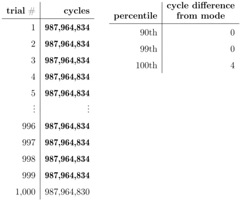
Running the workload on an isolated core via taskset -c 13 ./benchmark

gives the running times observed in Figure 3-10. Moreover, by consulting the per-formance counters for interrupts and exceptions, we can verify that our program was not interrupted during its execution. Therefore, it achieved complete ownership of its core.

(39)

trial # cycles 1 987,964,834 2 987,964,834 3 987,964,834 4 987,964,834 5 987,964,834 .. . ... 996 987,964,834 997 987,964,834 998 987,964,834 999 987,964,834 1,000 987,964,830 percentile cycle difference from mode 90th 0 99th 0 100th 4

Figure 3-10: Userspace runtimes on an isolated core demonstrating zero-cycle vari-ability.

3.10 Branch Prediction

The next step is to replicate our zero-cycle variability in a more complicated workload, one that branches heavily. Branching (in conditionals, loops, and more) is present in virtually any meaningful piece of code, but, unfortunately, is difficult to reason about because modern CPUs make liberal use of branch prediction. Rather than waiting for a conditional value to evaluate completely before deciding which of the

true and false instruction streams to execute next, CPUs use a branch predictor to determine which of the two streams is more likely to be chosen.

Modern branch predictors use complicated prediction mechanisms that get better at predicting the same conditionals over time, meaning that a benchmark workload is likely to see gradually improving performance the more trials are executed. Branch predictors generally maintain a hardware cache of branch instructions indexed by

(40)

their address in memory, much like a data cache [18]. Designs vary and have many undocumented features, as clever branch predictors are critical to fast processors and thus are closely guarded intellectual property. In a simple branch predictor, each branch might simply have a 2-bit saturating counter of {weakly, strongly} × {taken, not taken}. More complicated designs might combine the most-recent history of branches taken globally with the most-recent history of the local branch being predicted, and use that as an index into a two-dimensional table of counters, which gives sensitivity to overarching patterns in branching [18].

The ARM Cortex-A72 processor on our a1.metal instances, for example, uses a 2-level global history-based direction predictor [19]. The precise details of how the 2-level prediction works, including any special enhancements on top of the generic 2-level prediction scheme, are undocumented. We note that obtaining a precise un-derstanding of the branch predictor would amount to reverse engineering it, and would be a research publication in its own right.

The fact that the branch predictor gets more accurate the more a piece of code is executed makes it difficult to obtain consistent performance. Every time a piece of code executes, it might run a little faster because there are more correct branch predictions.

For our simple testcase, however, we find that a few warmup executions of the code under test are enough to put the branch predictor into a consistent state, giving zero-cycle variability in performance thereafter.

3.10.1 Branch-Heavy Workload

A new benchmark workload is necessary, one that makes liberal use of branching. The workload used in our previous testing, Figure 3-1, had only a single branch – the

b.ne instruction in Figure 3-2 that corresponds to the boundary condition of the

for-loop in Figure 3-1. This branch is highly predictable right from the start and consequently, as seen by the immediate zero-variability performance in Figure 3-6 and Figure 3-10, the branch predictor requires no warming up. To make heavy use of harder-to-predict branching, we devise a new workload.

(41)

A prime number sieve is a good example of a CPU-bound workload that has many difficult-to-predict branches. The C code of our sieve is shown in Figure 3-11, with the corresponding assembly shown in Figure 3-12. Note the large number of branch instructions in Figure 3-12. The branches are hard-to-predict because on each iteration of the outer loop (line 3) the internal divisibility branch (line 6) acts differently, which leads to many possible combinations of branch history that might be used in the 2-level prediction scheme. Therefore, it is a reasonable assumption that several executions of cpu_workload_branch() are necessary to fully prime the branch predictor.

1 int cpu_workload_branch(void){

2 int numPrimes = 0;

3 for(int num = 3; num < 6000; num++){

4 int divisor;

5 for(divisor = 2; divisor < num; divisor++){

6 if (num % divisor == 0){ 7 break; 8 } 9 } 10 if (divisor >= num){ 11 numPrimes++; 12 } 13 } 14 15 return numPrimes; 16 }

Figure 3-11: Implementation of a prime number sieve, an example of CPU-bound code with heavy branching.

(42)

1 +0: <cpu_workload_branch>: // label

2 +0: mov w3, #0x3 // data move

3 +4: mov w0, #0x0 // data move

4 +8: mov w4, #0x1770 // data move

5 +12: nop // no-op

6 +16: mov w1, #0x2 // data move

7 +20: nop // no-op

8 +24: udiv w2, w3, w1 // unsigned division

9 +28: msub w2, w2, w1, w3 // multiply-subtract

10 +32: cbz w2, 0x44 <cpu_workload_branch+68> // compare-branch-if-zero 11 +36: add w1, w1, #0x1 // add

12 +40: cmp w1, w3 // compare

13 +44: b.ne 0x18 <cpu_workload_branch+24> // branch-if-not-equal

14 +48: add w0, w0, #0x1 // add

15 +52: add w3, w3, #0x1 // add

16 +56: cmp w3, w4 // compare

17 +60: b.ne 0x10 <cpu_workload_branch+16> // branch-if-not-equal

19 +68: cmp w3, w1 // compare

20 +72: b.gt 0x34 <cpu_workload_branch+52> // branch-if-greater-than

21 +76: b 0x30 <cpu_workload_branch+48> // branch

Figure 3-12: The assembly corresponding to Figure 3-11.

3.10.2 Zero-Cycle Variability via Branch Predictor Warmup

We manage to obtain zero-cycle variability for our branch-heavy workload the same way that we did for the light workload in Section 3.9. We run the branch-heavy workload in the same environment.

Figure 3-13 contains the results of running our workload on an isolated core. We can see that the running times are at first inconsistent, but appear to slowly converge to a running time of 15,400,377 cycles, maintained for every subsequent run through the end. The table contains two additional datapoints per row: “predictable branches executed” and “mispredicted or non-predicted branches executed.” These values were read from performance counters BR_PRED and BR_MIS_PRED [13], and exactly track the cycles values in terms of converging to a consistent “steady state”

(43)

value. This convergence supports our hypothesis that the branch predictor needs several executions of cpu_workload_bench() before it maximally learns how to predict its branches, after which branches are predicted and mispredicted in exactly the same way on each execution, granting a consistent running time.

trial # cycles predictable branch exec. {mis,non}-predicted branch exec. 1 15,400,862 4,400,989 2,767 2 15,399,979 4,400,900 2,717 3 15,400,496 4,400,747 2,715 4 15,400,402 4,400,735 2,709 5 15,400,402 4,400,735 2,709 6 15,400,402 4,400,735 2,709 7 15,400,377 4,400,732 2,708 8 15,400,377 4,400,732 2,708 .. . ... ... ... 997 15,400,377 4,400,732 2,708 998 15,400,377 4,400,732 2,708 999 15,400,377 4,400,732 2,708 1,000 15,400,377 4,400,732 2,710 percentile cycle difference from mode 90th 0 99th 0 100th 486

(44)

3.10.3 Resetting the Branch Predictor

Resorting to “warming up” the branch predictor both wastes time on throwaway executions of the code and is unscientific. How many times does a particular workload need to be executed before the branch predictor is fully primed? Is it possible that the branch predictor history table alternates between several different states after each run, rather than converging to a single state? The answer will always depend on the peculiarities of the code and the branch predictor design, making it difficult to determine.

A better solution would be to reset the branch predictor before executing the workload. This would ensure that each execution incurs branch predictions and mis-predictions in the exact same deterministic way. Unfortunately, the Cortex-A72 pro-cessor on our a1.metal instances does not support flushing the branch predictor, only enabling/disabling it on boot via a processor control register. We attempted to sim-ulate flushing the branch predictor by running through thousands of autogenerated branch instructions between executions of our benchmark, but this proved unsuc-cessful, and a correct implementation likely requires a keener understanding of the branch predictor’s design. The most “correct” solution, therefore, would be flushing the branch predictor in a way specifically supported by the processor in question.

(45)

Chapter 4 𝜖 Variability in Memory Workloads

In this chapter, we confront variability in workloads that read and write data memory. Taming variability in CPU-bound workloads in Chapter 3 was an instructive starting point with impressive zero-cycle variability results, but virtually any real-world work-load will access memory, making it critical to address memory-related variability. We first present an overview of the memory subsystem (Section 4.1). We then investigate variability seen in workloads with working-sets that fit into L1 cache, L2 cache, and system memory (Section 4.3), showing that we can obtain less than 0.3% variability across thousands of trials of our memory benchmark under numerous different exe-cution parameters. Unfortunately, memory is a global resource, and our experiments demonstrate that a memory workload running on an isolated core can suffer interfer-ence from other cores in the system, making it difficult to obtain ultra-low variability (Section 4.4).

4.1 The Memory Subsystem

Understanding the hardware components of the memory subsystem, and how operat-ing systems manage memory, is crucial for reasonoperat-ing about memory-related variability. This section summarizes the main parts.

(46)

4.1.1 Virtual Memory

Processes access data in memory by a virtual, rather than physical, address. For example, a process accessing data located at address 0x00F0 in the physical memory chip might actually access it via address 0xAAF0 or 0xBBF0. Each process has a separate virtual-to-physical address mapping as any two processes can access the exact same virtual addresses; this mapping is called a “page table,” and is managed by the kernel. The memory management unit (MMU) is a hardware component responsible for translating virtual addresses to physical addresses on the fly by looking them up in the currently loaded page table.

4.1.2 Translation Lookaside Buffer

Many CPUs cache virtual-to-physical address translations in a translation lookaside buffer (TLB) to amortize the cost of address translation, which can be expensive due to the multiple levels of indirection in the page table (generally implemented as a 2-level tree for 32-bit machines and a 4-level tree for 64-bit). The TLB has to be kept in-sync with the current page table, meaning that its entries must be updated if the underlying page table entries change. For example, if a page is shared across multiple processors and its physical location changes, then its entry in all page tables must be updated and the corresponding TLB entry invalidated – this process is called a “TLB shootdown.”

4.1.3 Memory Caches

Memory is accelerated via hardware caches, which have small capacities but signifi-cantly faster access latencies than main memory. Caches operate on the empirically observed phenomenon of temporal and spacial locality.

Temporal locality implies that a piece of data read by the processor is likely to be read again in a short period of time – for example, a function might access the same variables and buffers multiple times. Spacial locality implies that the processor is likely to operate on adjacent memory, as when iterating through a buffer or accessing

(47)

various parts of a large data structure represented sequentially in memory.

Caches cater to both of these access patterns. They account for temporal locality by storing recently accessed blocks of data until they are evicted by many new ac-cesses, so the processor is likely to read data from cache when repeatedly accessing the same memory. Caches account for spatial locality since each cache line is often larger than an individual memory access. Cache lines are generally 64 bytes wide, meaning that after an initial access to one part of the cache line, accesses to any other parts of the same line will use the cache rather than accessing main memory. Hardware pre-fetchers further accommodate spatial locality by identifying patterns in memory accesses and pre-fetching memory likely to be accessed next.

4.1.4 Cache Coherence

Multi-core processors have multiple data caches, which must be synchronized with one another to maintain a single coherent view of memory. This synchronization is carried out through a cache coherence protocol, like MESI, MOESI, or variants [20]. Depending on the particular protocol and hardware implementation, cache coherency may involve messages exchanged between caches (for example, when one core modi-fies a memory location in its cache that is currently present in other cores’ caches). It is difficult to speak generally about the performance interference implications of cache coherence, but it is conceivable that cache coherence traffic is present almost constantly in a system (even if memory is not shared), and thus interferes with mem-ory performance, due both to congesting chip buses and requiring caches to process it.

4.1.5 Memory Bandwidth

Finally, both latency and throughput affect memory performance. While some mem-ory accesses may well occur in parallel, a sudden burst of accesses may saturate the memory controller and slow one another down. Moreover, memory has a limited bandwidth, meaning that two processes with intensive memory activity will limit one

(48)

another’s performance. Therefore, any memory activity on our system, no matter the core that it originates from, may interfere with the performance of our benchmark – even if the benchmark runs on an otherwise isolated core.

4.2 Memory Benchmark

Investigating memory variability requires a benchmark that actually accesses memory, unlike the benchmark programs used in Chapter 3.

Figure 4-1 contains the code for our workload, along with the accompanying as-sembly in Figure 4-2. It accepts a buffer along with a number of accesses to per-form, which allows us to investigate variability both as a function of the size of the working-set, and the running time (proxied via the number of accesses). The func-tion performs random accesses to the supplied buffer. Random accesses are critical because sequential accesses are easily detected by the hardware prefetcher, which will prefetch upcoming memory accesses into L1 and L2 caches before they actually occur. It is then impossible to study variability in L2 and DRAM accesses because, even if our benchmark uses a buffer much larger than the cache sizes, most accesses will hit in L1 cache [21]. Random accesses subvert the prefetcher, letting us ensure that the workload hits entirely in L1 cache, L2 cache, or goes to DRAM, by using a sufficiently large buffer.

Note that we implement our own pseudorandom number generator (PRNG) in

custom_rand(). Using a handwritten PRNG instead of deferring to rand() in the C standard library gives us tighter control over exactly what code our benchmark executes, which is important when studying ultra-low variability. The actual PRNG implementation is taken directly from the GNU standard library source code [22]. Moreover, note that in Figure 4-2, the call to custom_rand() is simply inlined into

(49)

1 uint64_t custom_rand(uint64_t *state){

2 uint64_t newVal = ((*state * 1103515245U) + 12345U) & 0x7fffffff; 3 *state = newVal;

4 return newVal;

5 } 6

7 int cpu_workload_memory(char *buf, size_t size, int numIterations){

8 unsigned long long x = 0;

9 uint64_t state = 1;

10 for(size_t blockNum = 0; blockNum < numIterations; blockNum++){

11 x = ((x ^ 0x123) + buf[custom_rand(&state) % size] * 3) % 123456;

12 }

13 return x;

14 }

(50)

1 +0: cpu_workload_memory: //

2 +0: sxtw x2, w2 // signed extend

3 +4: cbz x2, 0x1070 <cpu_workload_memory+128> // cmp-branch-if-zero 4 +8: mov x8, #0x6301 // data move

5 +12: mov x12, #0x4e6d // data move

6 +16: movk x8, #0x78e6, lsl #16 // data move

7 +20: mov x7, #0xe240 // data move

8 +24: movk x8, #0x2ba9, lsl #32 // data move

9 +28: mov x4, #0x1 // data move

10 +32: mov x6, #0x0 // data move

11 +36: mov x3, #0x0 // data move

12 +40: movk x12, #0x41c6, lsl #16 // data move

13 +44: mov x11, #0x3039 // data move

14 +48: mov x10, #0x123 // data move

15 +52: mov w9, #0x3 // data move

16 +56: movk x8, #0x43f, lsl #48 // data move

17 +60: movk x7, #0x1, lsl #16 // data move

18 +64: madd x4, x4, x12, x11 // multiply-add 19 +68: eor x3, x3, x10 // exclusive-or 20 +72: add x6, x6, #0x1 // add 21 +76: and x4, x4, #0x7fffffff // add 22 +80: cmp x6, x2 // compare 23 +84: udiv x5, x4, x1 // unsigned-divide 24 +88: msub x5, x5, x1, x4 // multiply-subtract

25 +92: ldrb w5, [x0, x5] // load register byte

26 +96: umaddl x5, w5, w9, x3 // unsigned mult.-add

27 +100: lsr x3, x5, #6 // logical shift

28 +104: umulh x3, x3, x8 // unsigned multiply

29 +108: lsr x3, x3, #5 // shift right

30 +112: msub x3, x3, x7, x5 // multiply subtract

31 +116: b.ne 0x1030 <cpu_workload_memory+64> // branch-not-equal

32 +120: mov w0, w3 // data move

34 +128: mov w0, #0x0 // data move

(51)

4.3 L1, L2, DRAM variability

We investigate and compare the variability seen in accesses to L1 cache, L2 cache, and DRAM. An easy method of approximating accesses to “only” L2 cache, for example, is using a working-set size substantially larger than the size of L1 cache (32KB), but still smaller than the size of L2 cache (2,048KB). For example, random accesses to a buffer 2,000KB in size will, probabilistically speaking, almost always miss in L1 cache but hit in L2 cache.

Figure 4-3: Runtimes (with very tight error bars) for 300 trials of each of many combinations of number of memory accesses and working-set size. Note: logarithmic scale.

Figure 4-3 shows our first attempt at understanding memory performance and variability. Each point on the plot represents a particular combination of number of memory accesses and working-set size. Note the logarithmic scale on the x-axis. Points labeled “1x iterations” represent executions of the benchmark program with 1, 0242 memory accesses, those labeled “2x” had twice as many, and so on.

We can draw several conclusions about access times to the different tiers of mem-ory (L1 cache, L2 cache, and DRAM), the impact of TLB misses, and fixed costs

(52)

associated with longer running times.

There is a distinct, consistent execution time for accesses to L1, L2, and DRAM. The plateaus at working-sets of size <32KB, just below 2MB, and just above 2GB appear to confirm that, at least at the extremes, we obtain predominantly accesses to L1 cache, L2 cache, and DRAM. The gradual ramp-up in running time – i.e. the fact that each plot appears smooth rather than like a step function – is likely due to the fact that some accesses still hit in the the next lower cache. For example, all working-sets less than 32KB in size have an essentially constant running time because the best- and worst-case access time is that of L1 cache. Once the working-set size exceeds 32KB, running time immediately increases because some accesses go to L2 cache. However, for a working-set of size 33KB, for example, a majority of accesses will still hit in L1, meaning that the total running time will be closer to the steady-state running time for L1 accesses than L2 accesses. Hence the gradual increase towards a plateau at larger sizes, rather than a step-function behavior.

The middle plateau of running times of DRAM accesses, for working-set sizes between 32MB and 512MB, likely occurs due to the TLB overflowing. At the end of the plateau around 256MB, it’s likely that all memory accesses go to DRAM but all page address translations hit in TLB. Past 256MB, TLB misses start occuring, causing another uptick in execution time. Similar results are seen in the work of Drepper [21].

Increasing the number of iterations scales the running time exactly proportionally, implying there are no substantial hidden costs to a longer execution. For example, the “2x” plot is exactly the “1x” plot scaled up by a factor of 2 with a very small error margin.

The variability seen within each trial is less than 0.3%. Sample variabilities are shown in Table 4.1. The general trend is increasing variability for higher tiers of memory, but this is not always the case. Our testing occasionally demonstrates high variability in L1 cache, for example, possibly because it is more substantially affected by some kinds of cross-core interference than either L2 or DRAM.

(53)

working-set size 90th % 99th % max % L1 Cache 0.00% 0.00% 0.00% L2 Cache 0.01% 0.01% 0.01% DRAM 0.09% 0.11% 0.11%

Table 4.1: Variability of 16x iterations for different working-set sizes.

4.4 Interference from Other Cores

We demonstrate that, unlike with a CPU-bound workload, we cannot fully isolate our memory workload from other cores. This is due to the fact that memory is a global resource shared by all cores, with common buses, memory chips, etc., unlike the execution units of a core, which are used only by that core. It may be possible to achieve a degree of isolation on a NUMA system, where memory is composed of distinct physical blocks with affinities for specific CPUs, but there is no clear means of isolating a chunk of memory on our UMA (Uniform Memory Access) system.

4.4.1 Interference Case Study: Lightweight User Script

Our first example occurred during experimentation due to an innocuous user config-uration script, and clued us into the existence of universal cross-core interference.

Figure 4-4 shows the running times of our memory benchmark for a buffer that fits comfortably in L1 cache. The otherwise consistent running times are punctuated by regularly occurring spikes. These spikes occur at an interval of roughly 2 seconds. We initially tried identifying the issue by observing performance counters, but these sim-ply show the consequences of the root cause (in cache misses, etc.) rather than hinting at what that cause might be. We ultimately deduced the culprit by inspecting system scheduler activity, recorded via the perf sched tool, which showed that some user configuration scripts related to tmux, a terminal multiplexer, were running exactly once every 2 seconds. Removing them removed the spike from our running time. Of course, due to our use of isolcpus (Section 3.6.1), the scripts were running not only

(54)

on a different core, but on a different core cluster, with its own L2 cache. Moreover, each core has its own L1 cache and our workload used a buffer that fit comfortably inside it, which made the interference even more confusing – we expected essentially no interference from the rest of the system. It is not immediately clear why memory activity on an unrelated core was affecting a largely L1 workload on our otherwise quiet benchmark core. This phenomenon hints at the highly interconnected nature of memory. Even though our benchmark core owns its own L1 cache, it is possible that the cache periodically writes back to memory, which would be negatively impacted by other memory load in the system. Or maybe other memory activity down-clocked the memory subsystem. Or maybe there were TLB shootdowns involved.

Figure 4-4: Running times of L1 Cache benchmark demonstrating intermittent interference due to user script running on unrelated core.

4.4.2 Interference Case Study: Memory Intensive Workload

Section 4.4.1 suggested that even an innocuous user process may cause cross-core interference, so let us investigate a worse-case scenario with a memory-intensive program running on another core. Figure 4-5 shows the results of running our

(55)

random-access benchmark on a quiet core, with and without intermittent interfer-ence. We simulate intermittent interference by running the same benchmark peri-odically on a distant core, hence the intermittent spikes in performance. Without interference, the benchmark experiences a 90th/99th/100th-percentile variability of 0.02%/0.03%/0.03%; with interference, that variability increases to 1.31%/1.33%/1.34%.

Figure 4-5: Performance variability with and without intermittent interference.

4.4.3 Mitigating System Activity

Sections 4.4.1 and 4.4.2 demonstrates that we cannot match the ultra-low variability of a CPU workload with a memory workload because of the highly interconnected nature of memory, and the resulting cross-core interference.

An ideal solution would be to temporarily “lock” all cores on the machine and prevent all other processes from running while our benchmark executes. This global lock can be easily simulated by writing our benchmark into a kernel module again and running it on all cores via the on_each_cpu() kernel method. On a single core, the kernel module would execute the benchmark, and on all others, it would simply exe-cute a busy-spin loop. However, an early attempt suggested that the kernel prevents

(56)

this code from running on all cores exactly simultaneously, and will defer the execution of the on_each_cpu() code on at least one core until it finishes execution on an-other core. This may be a mechanism to avoid global lockup – unfortunately, global lockup is exactly what we want to achieve. Even beyond this one-core exception, Linux has a host of anti-lockup mechanisms that dislike a long-running benchmark with interrupts disabled, and thus trigger for our long-running performance tests.

A practical, if imperfect, strategy to mitigate interference is to simply strip down the system as much as possible by removing unnecessary processes. Cross-core in-terference is simply unlikely if there is almost nothing running. This strategy also applies to CPU-bound workloads, as discussed in Section 3.6.3. Consultation of top

and ps shows a large number of processes running even on our quiet system, many of which are unnecessary. Moreover, lsmod lists all currently loaded kernel modules, some of which can be disabled.

Lastly, it may be easy to modify the Linux kernel source code to run kernel workers and other threads less frequently, or to simulate the aforementioned global lock. However, these changes would require a more intimate understanding of kernel internals, and would be one-off and not very portable.

(57)

Chapter 5 Quiescing a System

This chapter refines the experimental results and conclusions of the preceding chapters into a list of actionable steps for quiescing a system for low-variability performance. Section 5.1 summarizes major sources of variability and corresponding mitigation strategies. Section 5.2 discusses limitations to those strategies and identifies sources of variability that are practically unavoidable without deep changes to the system.

5.1 Actionable Steps

There are several “actionable” steps that make huge impacts on performance variabil-ity, including: removing DVFS, disabling simultaneous hyperthreading, and more. A step is “actionable” if it is officially supported by the operating system and can be taken with minimal effort.

5.1.1 DVFS

Processors with Dynamic Voltage and Frequency Scaling (DVFS) can scale their clock frequency up and down. DVFS allows for reduced power consumption when there is no work to be done – the processor will scale down the frequency when a core has no scheduled work, and rapidly scale it back up when work appears. Similarly, the processor may scale down its frequency to prevent over-heating, for example when all

(58)

cores are busy and generating excessive heat.

Unfortunately, DVFS can introduce performance variability because of the time taken to ramp up a core to its maximum operating frequency, as shown in Figure 5-1. This experiment was conducted on an AWS c5n.metal instance with Intel Xeon 8124M processors, which have DVFS enabled by default. The same benchmark was run twice, once with the performance governor (which manages DVFS) set to a pow-ersave configuration, and once with a performance configuration. As the names imply, the powersave configuration aggressively reduces the clock frequency when cores are idle in order to reduce power consumption, and the performance configu-ration essentially keeps the cores running at their maximum clock frequency all the time. When run under the powersave configuration, our benchmark exhibits a slow “warmup” as the processor clock frequency increases from 1.2GHz (its idle frequency) to 3.5GHz (its maximum frequency). The processor steps through several discrete frequencies, hence the step behavior in the plot. Under the performance configura-tion, on the other hand, the processor is always running at its maximum frequency, so there is no equivalent warmup period. Thus, DVFS, as shown under the powersave configuration, can massively skew performance numbers for certain trials, and should be disabled for low-variability/high-performance use-cases.